Theory and simulation for equilibrium glassy dynamics in cellular Potts model of confluent biological tissue
Abstract
Glassy dynamics in a confluent monolayer is indispensable in morphogenesis, wound healing, bronchial asthma, and many others; a detailed theoretical framework for such a system is, therefore, important. Vertex model (VM) simulations have provided crucial insights into the dynamics of such systems, but their nonequilibrium nature makes it difficult for theoretical development. Cellular Potts model (CPM) of confluent monolayer provides an alternative model for such systems with a well-defined equilibrium limit. We combine numerical simulations of CPM and an analytical study based on one of the most successful theories of equilibrium glass, the random first order transition theory, and develop a comprehensive theoretical framework for a confluent glassy system. We find that the glassy dynamics within CPM is qualitatively similar to that in VM. Our study elucidates the crucial role of geometric constraints in bringing about two distinct regimes in the dynamics, as the target perimeter is varied. The unusual sub-Arrhenius relaxation results from the distinctive interaction potential arising from the perimeter constraint in such systems. Fragility of the system decreases with increasing in the low- regime, whereas the dynamics is independent of in the other regime. The rigidity transition, found in VM, is absent within CPM; this difference seems to come from the nonequilibrium nature of the former. We show that CPM captures the basic phenomenology of glassy dynamics in a confluent biological system via comparison of our numerical results with existing experiments on different systems.
I Introduction
Collective motion of cells in a confluent monolayer is important in morphogenesis Friedl and Gilmour 2009; Tambe et al. 2011; Malmi-Kakkada et al. 2018, cancer metastasis Malmi-Kakkada et al. 2018; Streitberger et al. 2020, wound healing Poujade et al. 2007; Brugués et al. 2014; Noppe et al. 2015; Das et al. 2015, bronchial asthma Park et al. 2015; Atia et al. 2018, vertebrate body axis elongation Mongera et al. 2018, and many others. Recent experiments Angelini et al. 2011; Malinverno et al. 2017; Palamidessi et al. 2019; Park et al. 2015; Mongera et al. 2018; Garcia et al. 2015; Malmi-Kakkada et al. 2018 have shown the dynamics in such cellular systems has remarkable similarities with that of a glassy system. Glassy dynamics refers to the extreme slowing down, of the order of 12-14 orders of magnitude, with a small change of control parameter without any discernible structural signature or phase transition Debenedetti and Stillinger 2001; Berthier and Biroli 2011. The key characteristics of a glassy system, such as the complex stretched exponential relaxation Malinverno et al. 2017; Park et al. 2015; Atia et al. 2018, the growing dynamic heterogeneity characterized through higher order susceptibilities Palamidessi et al. 2019; Park et al. 2015; Atia et al. 2018; Angelini et al. 2011, non-Gaussian nature of the displacement distribution Giavazzi et al. 2018, etc, are also displayed in the collective dynamics of cellular systems. Importance of the problem calls for a detailed theoretical framework for the glassy dynamics in such systems. A confluent monolayer of cells is different from particulate systems in at least two crucial aspects: first, the packing fraction is always unity, and, thus, can not be a control parameter Bi et al. 2015; Bi et al. 2016, second, the inter-particle interaction potential can be varied as a function of the control parameter.
Inspired by the physics of soap bubbles, vertex models Honda 1978; Bock et al. 2010 that represent individual cells by polygons have provided important insights into the dynamics of such systems Farhadifar et al. 2007; Staple et al. 2010; Fletcher et al. 2014; Bi et al. 2015; Bi et al. 2016; Barton et al. 2017; Sussman et al. 2018; Krajnc et al. 2018; Henkes et al. 2020. Within vertex models, the vertices of the polygons are evolved with certain rules. The cellular perimeter between vertices is either straight by construction or has a constant curvature, whereas in experiments it can deviate arbitrarily from a straight line Mitchel et al. 2020; Bock et al. 2010; Atia et al. 2018; how this deviation affects the dynamics remains unknown. An important process governing dynamics in a confluent cellular monolayer is the transition or the neighbor exchange process Fletcher et al. 2013; Fletcher et al. 2014; where an edge between two cells shrink to zero and a new one appears perpendicular to it (see Fig. 1(a) for a schematic illustration). Within vertex models, this process is implemented by a perpendicular flip of an edge whenever its length becomes smaller than a predefined value, ; such an implementation necessarily makes the model nonequilibrium. Moreover, the dynamics crucially depends on Das et al. 2020, making extension of equilibrium theories for such systems nontrivial and an equilibrium variant of the model is important. Confluent systems have shown to exhibit some unusual glassy properties, understanding the dynamics of such systems should, therefore, also be interesting from the perspective of equilibrium glass transition theories.
The lattice-based cellular Potts models (CPM) Graner and Glazier 1992; Glazier and Graner 1993; Hirashima et al. 2017 define another important class of models for cellular dynamics and have been applied to single and collective cellular behavior Czirók et al. 2013; Magno et al. 2015; Rens and Edelstein-Keshet 2019; Kabla 2012, cell sorting Graner and Glazier 1992; Glazier and Graner 1993, dynamics on patterned surfaces Marée et al. 2007, gradient sensing Camley and Rappel 2017; Marée et al. 2007, etc. Despite the widespread applicability of CPM, its glassy aspects remain relatively unexplored. To the best of our knowledge, there exists only one such simulation study Chiang and Marenduzzo 2016, which however did not consider the perimeter constraint and, as we show below, models with and without this constraint are qualitatively different.
The primary difference between CPM and vertex-based models lies in the details of energy minimization Albert and Schwarz 2016. Two crucial aspects of CPM, however, make it advantageous over vertex-based models: it allows arbitrary shape of cell perimeters, and transitions are naturally included within CPM. This latter feature allows to study the dynamics of the model in equilibrium, which is the focus of this current study. Although biological systems are inherently out of equilibrium and activity is crucial, it is important to first understand the behavior of an equilibrium system in the absence of activity, which can be included later Nandi et al. 2018; Nandi 2018. Furthermore, we find that the dynamics in CPM is similar to that in a vertex model and the theoretical framework, developed here, can be applied to the results of vertex-based models Nandi et al 2020.
The dynamics of CPM in the glassy regime provides an alternative and complementary angle to vertex-models to understand the glassiness in confluent systems. Simulation studies of vertex models have established a rigidity transition that controls the glassy dynamics and the observed shape index (average ratio of perimeter to square root of area) has been interpreted as the structural order parameter of glass transition Park et al. 2015; Bi et al. 2015; Bi et al. 2016. We show that these results are not generic of confluent systems and, possibly, a consequence of the nonequilibrium nature of the vertex models. Our aim in this work is twofold: first, we bridge the gap in numerical results through detailed Monte-Carlo (MC) based simulation study of CPM in the glassy regime, and second, we develop the random first order transition (RFOT) theory Kirkpatrick and Thirumalai 2015; Lubchenko and Wolynes 2007, one of the most popular theories of glassy dynamics in particulate systems, for a confluent system.
The results of the current work can be summarized as follows: (i) We simulate CPM for a confluent system in glassy regime and find that the qualitative behaviors of the dynamics are similar to those in vertex models. (ii) The target perimeter that parameterizes the interaction potential, plays the role of a control parameter. Geometric restriction brings about two regimes as is varied; dynamics depends on in the low- regime and is independent of in the other, large- regime. (iii) One striking result of our study is the presence of glassy behavior in the large- regime, where vertex models show absence of glassiness, (iv) The rigidity transition of vertex models is absent within CPM; this possibly comes from the difference of how transitions are included within the two models. (v) We develop RFOT theory for confluent systems and the theory agrees well with our simulation results. (vi) The perimeter constraint is crucial for the unusual sub-Arrhenius behavior and the system being confluent alone is not sufficient for such behavior. (vii) Velocity distribution is non-Gaussian in the glassy regime in agreement with existing experimental results. The rest of the paper is organized as follows: We introduce CPM in Sec. II and describe some basic characteristics of the system in Sec. III. The main results of the work, development of RFOT theory for confluent systems and simulation results in low- and large- regimes are presented in Sec. IV. We show some critical tests of our theory in Sec. V and comparison with experiments in Sec. VI. Finally, we conclude the paper in Sec. VII via a discussion of our results.

II Cellular Potts Model
The cellular Potts model (CPM), also known as the “extended large- Potts model” or the “Glazier-Graner-Hogeweg (GGH) model” Graner and Glazier 1992; Glazier and Graner 1993; Hogeweg 2000, is a lattice based model to simulate the behavior of cellular systems Hirashima et al. 2017; Marée et al. 2007; Graner and Glazier 1992. For the CPM in , we use a square lattice of size to represent a confluent cell monolayer. Each cell in this lattice consists of a set of lattice sites with the same integer Potts spin (), also known as cell index, where , being the total number of cells; is usually reserved for fluid that is absent in our model. The cells in this model are evolved by stochastically updating one lattice site at a time through Monte Carlo (MC) simulation via an effective energy function Hirashima et al. 2017; Albert and Schwarz 2016:
| (1) |
where are cell indices, is the total number of cells, and are area and perimeter of the th cell, and are target area and target perimeter, chosen to be same for all cells. and are elastic constants related to area and perimeter constraints. The summation in the last term is taken over all nearest neighbor sites , is the Kronecker delta function. gives the strength of inter-cellular interaction, positive values of signify repulsion whereas negative represents attractive interaction.
Cells can be treated as incompressible in Prost et al. 2015. It has been found in experiments that the height of a monolayer remains almost constant Farhadifar et al. 2007. These two findings together allows a description of the system with an area constraint leading to the first term in Eq. (1); gives the target cell area and determines the strength of area fluctuation from . On the other hand, mechanical properties of a cell is mostly governed by cellular cortex Prost et al. 2015 and this can be encoded in a perimeter constraint with a target perimeter in the form of the second term in Eq. (1), with determining the strength of perimeter fluctuation. Inter-cellular interactions through different junction proteins like E-Cadherins and effects of pressure, contractility, cell adhesion, etc can be included within an effective interaction term, the third term in Eq. (1). The last term in is proportional to and can be included within the second term with a renormalized value of , however, for ease of discussion we keep it separately. CPM represents the biological processes for dynamics through an effective temperature Graner and Glazier 1992; Hirashima et al. 2017; Durand and Heu 2019. Fragmentation of cells is forbidden Durand and Guesnet 2016 in our simulation to minimize noise. We mainly focus on the model with and get back to the model with and , that was simulated in Ref. Chiang and Marenduzzo 2016, later in the paper, in Sec. V.
III Basic Characteristics of the dynamics
We next describe some basic characteristics of the dynamics in a confluent system from the perspective of our numerical study of CPM.
Dynamics is independent of : When total area of the system is fixed, in Eq. (1) becomes independent of . The change in energy coming from the area term alone for an MC attempt between th and th cells is that is independent of . Since dependence of dynamics can only come through , the dynamics becomes independent of . This argument can also be extended for a polydisperse system. The input shape index, , therefore, cannot be a control parameter for the dynamics and should be viewed as a dimensionless perimeter; this result was also found for voronoi model dynamics Yang et al. 2017. , on the other hand, parameterizes the interaction potential and plays the role of a control parameter.
Two different regimes of : The observed shape index, , where denotes average over all cells, tends to a constant with decreasing (Fig. 1b). seems to be the structural order parameter of glass transition in vertex models Park et al. 2015; Bi et al. 2015; Bi et al. 2016, however, as we show below, such an interpretation is not applicable for CPM. for a fixed has a minimum value, , that depends on geometric constraints, here confluency and underlying lattice. When is below , of most cells cannot satisfy the perimeter constraint in Eq. (1) as they remain stuck around . At high fluid regime, when dynamics is fast, cell boundaries are irregular leading to larger values of and ; but, at low glassy regime, when dynamics is slow, cell boundaries tend to be regular leading to lower values of and . Figure 1(b) shows at three different as a function of ; decreases with decreasing at a fixed and saturates to (the quantitative value is lattice-dependent, however, the qualitative behavior, we expect, to be independent of the lattice). The lowest value of is dictated by the geometric restriction in the low- regime. Our interpretation is consistent with the simulation results in voronoi models Sussman et al. 2018; Sussman and Merkel 2018 as well as the fact that in a large class of distinctly different systems has similar values Li et al. 2020; Atia et al. 2018.
On the other hand, when , the large- regime, most cells are able to satisfy the perimeter constraint and the lowest value of is governed by , as deviation from costs energy. We show at the glass transition temperature, , (defined as the when relaxation time becomes ) as a function of in Fig. 1(c); tends to a constant in the low- regime whereas it increases linearly with in the large- regime. The geometric restriction is clearer in the plot of ; it decreases linearly with increasing in the low- regime and then tends to zero. The interfacial tension, defined as Magno et al. 2015, is non-zero along cell boundaries in the low- regime and becomes zero in the large- regime as increases.
transitions within CPM: Dynamics in a biological tissue proceeds via a series of complicated biochemical processes that are simply represented via an effective temperature within CPM Hirashima et al. 2017; Durand and Heu 2019. This is an extreme level of simplification from biological perspective, however, is convenient from theoretical aspects. At the coarse grained level, transitions where cells exchange their neighbors Fletcher et al. 2014 are crucial for dynamics in a confluent system. As discussed in the introduction, and illustrated in Fig. 1(a), implementation of transition within vertex models is nonequilibrium in nature. On the other hand, transitions are naturally included within CPM. We show two such transition processes from our simulations in Fig. (1(d)) for at (upper panel) and for at (lower panel). The transitions within CPM are equilibrium processes and their rates depend on and ; this crucial difference, compared to vertex models, is important from theoretical perspective as it allows a well-defined equilibrium limit of the model and makes it easier to extend equilibrium theories of glassy dynamics for confluent systems. More important, as discussed in Sec. IV, this difference of how transitions are implemented is, possibly, related to the absence of glassy dynamics in the large- regime as well as the identification of as the structural order parameter of glassy dynamics within the vertex models.

IV Results
We now present our theory for the glassy dynamics in a confluent monolayer. The simulation results for glassy dynamics within CPM, both in the low- and large- regimes, are presented along with the theory.
RFOT theory for CPM: The physics of glassy dynamics, even for particulate systems in equilibrium, continues to be debated leading to many different theories of glass transition Berthier and Biroli 2011; Hecksher and Dyre 2015. One of the most successful theories is the random first order transition (RFOT) theory due to Wolynes, Kirkpatrick and Thirumalai Kirkpatrick et al. 1989; Kirkpatrick and Thirumalai 2015; Lubchenko and Wolynes 2007; Bouchaud and Biroli 2004; Parisi and Zamponi 2010. Despite the intricate microscopic phenomenology, the theory leads to a simple set of predictions that agree well with experiments on wide set of glassy systems Lubchenko and Wolynes 2007; our goal in this work is to develop this theory for a confluent system to understand the effect of on the glassy dynamics.
Within RFOT theory, a glassy system consists of mosaics of different states; a nucleation-like argument gives the typical length scale of these mosaics Lubchenko and Wolynes 2007. Consider a region of length scale in dimension , the energy cost for rearrangement (changing state) of this region is
| (2) |
where is the decrease in energy per unit volume due to the rearrangement, and , volume and surface of a unit hypersphere, , the surface energy cost per unit area and is the exponent relating surface area and length scale of a region. Within RFOT theory, the drive to reconfiguration is entropic in nature and given by the configurational entropy, , that can be thought of as the difference of total entropy of the system and its entropy if it was allowed to crystallize. Thus, , where is the Boltzmann constant. Minimizing Eq. (2) with respect to , we get the typical length scale, , for the mosaics as
| (3) |
In general, the interaction potential, , of the system determines both and . Within CPM, the interaction potential is parameterized through , thus, . The temperature dependence of is assumed to be linear Wolynes and Lubchenko 2012, thus, and we write Eq. (3) as
| (4) |
where is a constant. Within RFOT theory, relaxation dynamics of the system refers to relaxations of individual mosaics. The energy barrier associated for the relaxation of a region of length scale is , where is an energy scale and is an exponent. The relaxation time then becomes , where is a microscopic time scale independent of , but can depend on interatomic interaction potential, hence, on . Taking , where is a constant Lubchenko and Wolynes 2007; Kirkpatrick and Thirumalai 2015 and setting to unity, we obtain as
| (5) |
Following Refs. Kirkpatrick et al. 1989; Kirkpatrick and Thirumalai 2015 we take and then Eq. (5) can be written as
| (6) |
where is another constant. The theory presented here is similar in spirit with that for a network material obtained by Wang and Wolynes Wang and Wolynes 2013. Eq. (6) gives the general form of RFOT theory for the CPM; we obtain the detailed forms of and for different systems and regimes that we consider below. Our approach is perturbative in nature and we look at the effect of by expanding the potential around a reference state.
Low regime: As discussed above, for most cells are less than in this regime. Figure 2(a) shows a typical configuration of cells and their centers of mass for a system, close to glass transition. The mean-square displacement () and the self-overlap function, , (defined in Appendix A) as a function of time show typical glassy behavior (Figs. 2b,c). We define relaxation time, , as .
We now develop the RFOT theory for CPM in this regime, where cells are not able to satisfy the perimeter constraint and the dynamics depends on . Within our perturbative approach we treat a confluent system with as our reference system around which we expand the effect of varying on and . Thus, we have
| (7) |
where and we have ignored higher order terms. Within RFOT theory, glassiness, that is the abrupt slowing down of dynamics at low , results from a thermodynamic transition taking place at an even lower , known as the Kauzmann temperature Kauzmann 1948, , where the configurational entropy of the system vanishes and diverges. Thus, can be written as
| (8) |
where is the difference of specific heats of the liquid and the periodic crystalline phase. Within linear order, , the change in potential due to a variation in from the reference state, can be taken to be proportional to :
| (9) |
Using Eqs. (IV-IV) in Eq. (6), we obtain
| (10) |
where , and are all constants. The value of depends on the average cell area, for the results presented in this work, the average cell area is 40 and we find provides a good description of the data. Thus, using , we obtain
| (11) |
The constants , , and are independent of and ; they only depend on the microscopic details of a system and dimension. For a given system, we treat these constants as fitting parameters in the theory and obtain their values from fit with simulation data. Note that depends on the high properties of the system, which is nontrivial and will be explored elsewhere. Our analysis in the low- regime shows that -dependence of is weaker and can be taken as a constant.
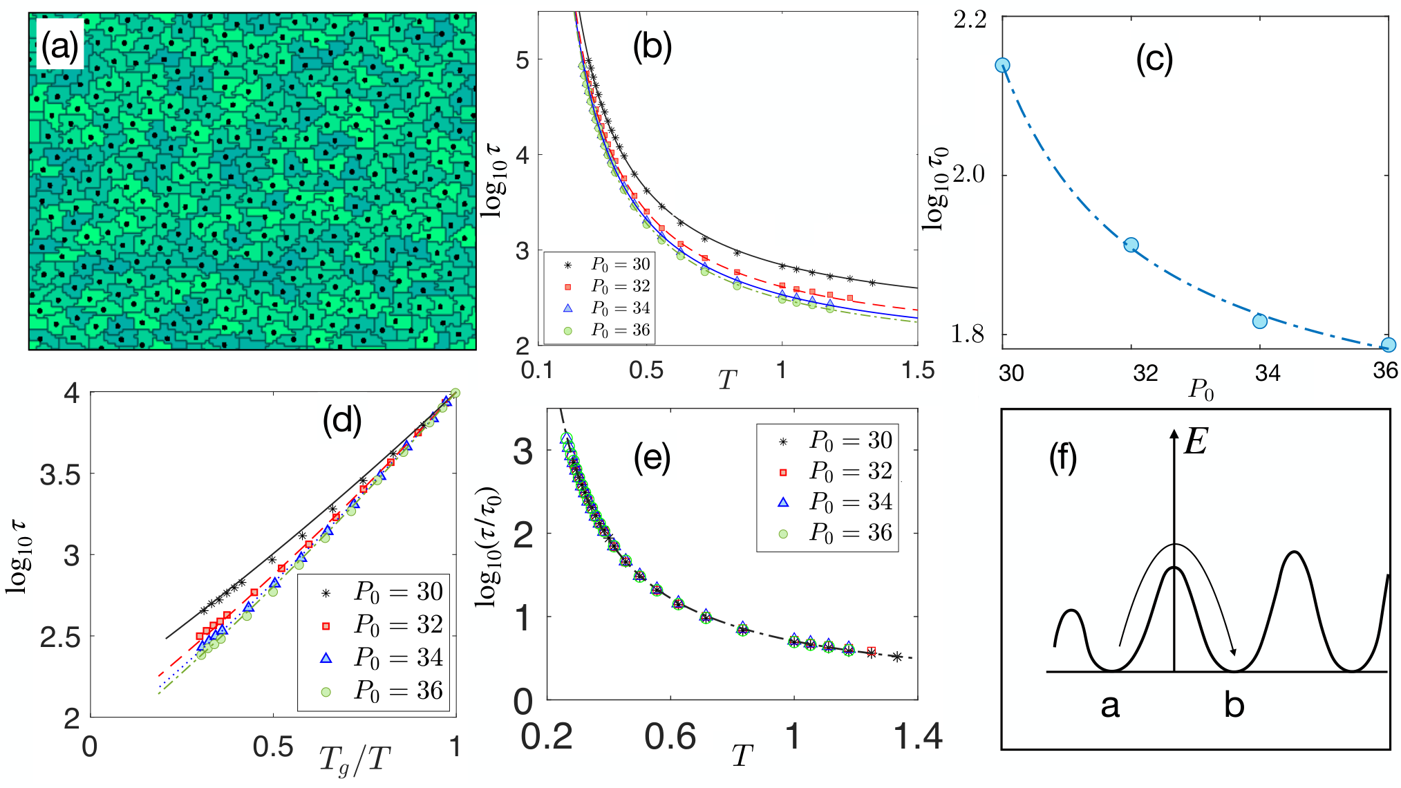
The minimum possible perimeter in our simulation is 26 (Appendix A) and we expect the critical separating the two regimes to be somewhere between 27 and 28. We first concentrate on the results for to and present as a function of for different in Fig. 2(d). We fit one set of data presented in Fig. 2(d) with Eq. (11) and obtain the parameters as follows: , , , and . Note that with these constants fixed, there is no other fitting parameter in the theory, we now show the plot of Eq. (11), as a function of for different values of with lines in Fig. 2(d). Figure 2(e) shows the same data in Angell plot representation that shows as a function of in semi-log scale. All the curves meet at by definition. The simulation data agree well with RFOT predictions at low where the theory is applicable.
When , where is a constant, we obtain a straight line in the Angell plot representation of , as in Fig. 2(e); this is the well-known Arrhenius behavior Berthier and Biroli 2011; Debenedetti and Stillinger 2001. Super-Arrhenius behavior, where changes faster than the Arrhenius law, leads to the relaxation time curves below this straight line whereas sub-Arrhenius behavior, that is slower than the Arrhenius law, shows up as the curves being above this line in Angell plot representation. In most equilibrium glassy systems, increases similar to or faster than Arrhenius law Lubchenko and Wolynes 2007; Berthier and Biroli 2011; Debenedetti and Stillinger 2001. One striking feature of the Angell plot in Fig. 2(e) is the sub-Arrhenius nature of . Similar results were reported for voronoi and vertex models in Refs. Sussman et al. 2018; Li et al. 2021 demonstrating similarities between CPM and vertex-based models. Within our RFOT theory, the sub-Arrhenius relaxation appears due to the distinctive interaction potential imposed by the perimeter constraint, in a regime controlled by geometric restriction, and appears when the system is about to satisfy the perimeter constraint. An important characteristic of this regime is that becomes negative. We get back to this point in Sec. V when we subject our RFOT theory to more stringent tests.
One can define a kinetic fragility, , and fit the simulation data for different with the form . We present in Fig. 2(f) where symbols are values obtained from fits with simulation data and the dotted line is theoretical prediction, the agreement, again, is remarkable. Fragility of the system decreases as increases and becomes more negative consistent with stronger sub-Arrhenius behavior.
Large- regime: In this regime most cells satisfy the perimeter constraint, cell boundaries are nonlinear [Fig. 3(a)], and dynamics becomes independent of implying constant values of and . Then the RFOT theory, Eq. (6) after a straightforward algebra, becomes
| (12) |
Although on the average, there are fluctuations of around when . The interaction potential is governed by these fluctuations that are stronger at higher . Thus, -dependence of is important in this regime.
Figure 3(b) shows as a function of ; they clearly vary for different and this difference comes from -dependence of . We fit Eq. (12) with one set of data and obtain , and a corresponding value for . Keeping and fixed, we next fit rest of the data to obtain . The fits are shown by lines in Fig. 3(b) and is shown in Fig. 3(c) where the line is a proposed form: . Figure 3(d) shows the Angell plot representation of the same data as in (b) and lines are the corresponding RFOT theory plots. Figure 3(e) shows as a function of for different values of , all the data following a master curve support our hypothesis that -dependence in this regime comes from .
More important, one would expect no glassy behavior in this regime if a rigidity transition, as in the vertex model Bi et al. 2015; Bi et al. 2016, controlled glassiness . In contrast, CPM shows the presence of glassy behavior even in this regime, where at is proportional to [Fig. 1(c)], thus, cannot be an order parameter for the glass transition in CPM. As apparent from Fig. 3(a), the configuration in this regime is disordered; at strictly zero , the minimum energy of the system is zero as cells are able to satisfy the area and perimeter constraints. However, the ground state is degenerate with a large multiplicity Staple et al. 2010. Dynamics in this regime can be viewed as exploration of the system among these equal energy ground state configurations. Consider two such states, shown by and in a schematic energy landscape plot Debenedetti and Stillinger 2001 in Fig. 3(f). The energy difference between the states is zero, but they are separated by a barrier; any dynamics necessarily requires change in area, even for the moves where perimeter can be kept constant, leading to a barrier. Within vertex model, the nonequilibrium implementation of transitions may allow transition between two such states (going from (i) to (iii) in Fig. 1(a)) without a cost; this is, possibly, the source of dynamics even at zero , leading to the rigidity transition. However, the absence of this nonequilibrium process within CPM forbids any dynamics at strictly zero as barrier crossings are not allowed; this rules out the rigidity transition of vertex models Bi et al. 2015 in CPM. In contrast to the vertex models, this rigidity transition is also absent in equilibrium voronoi models Sussman et al. 2018; Sussman and Merkel 2018, the source of this difference remains unclear. A more detailed understanding of the effect of the transitions in vertex models is outside the scope of the current work.
V Further tests of extended RFOT theory
Having demonstrated that our RFOT theory captures the key characteristics of glassiness in a confluent system, we now subject our theory to stringent tests through three different questions:
Within the theory sub-Arrhenius behavior is found when the effective is negative, i.e., (Eq. (11)). This implies super-Arrhenius behavior for . We now simulate the system in this regime and show the Angell plot in Fig. 4(a) where symbols represent simulation data and the corresponding lines are RFOT theory predictions. We emphasize that these curves are not fits, we simply plot Eq. (11) with the constants as obtained earlier. All the relaxation curves for different are super-Arrhenius as predicted by the theory. Ref. Li et al. 2021 show super-Arrhenius behavior in voronoi model simulations in the low- regime, consistent with our theory. Figure 4(b) shows comparison of , obtained from simulation and RFOT theory, for different .
Next, we illustrate that the sub-Arrhenius behavior and negative kinetic fragility is a result of the perimeter constraint in Eq. (1) and confluency alone is not enough for such behavior. We simulate a confluent system with and study the glassy behavior as a function of (Eq. 1). Considering the reference system at a moderate value of , a similar calculation as above gives the RFOT expression for as
| (13) |
where , , and are constants. Fitting Eq. (13) with simulation data for , we obtain , , and . Figure 4(c) shows simulation data for as a function of for different (symbols) as well as the corresponding RFOT theory (Eq. 13) predictions (lines). The Angell plot corresponding to these data are shown in Fig. 4(d). The system exhibits super-Arrhenius relaxation and data for different follow a master curve, in agreement with theory. These results are important from at least two aspects: first, they show that systems with and without the perimeter constraint are qualitatively different Chiang and Marenduzzo 2016, and second, that the presence of the perimeter constraint is crucial for the sub-Arrhenius behavior of the system.

Finally, we compare the stretching exponent Gupta et al. 2020; Xia and Wolynes 2001 that describes decay of the overlap function . The RFOT expression for (Appendix B) is
| (14) |
where and are two constants; we fit Eq. (14) with the simulation data for , as shown in Fig. 4(e), and obtain and . We then compare the RFOT predictions with simulation data for different as shown in Fig. 4(f) for four different . Again, the trends for agree quite well with theoretical predictions.
VI Comparison with experiments
We now demonstrate the applicability of CPM to biological systems through comparison of theoretical predictions with existing experimental data. Instead of a detailed comparison with a particular system, as is common for biophysical modeling, our aim here is to illustrate that CPM captures the key characteristics of dynamics in a wide class of confluent cellular monolayer. An important characteristic of glassiness is the non-Gaussian nature of the van-Hove function, , which is the probability distribution of displacements, within time , of the constituent cells in the system, defined as
| (15) |
where the averaging is over all cells and . is Gaussian at small and deviates from the Gaussian behavior at large as shown in Fig. 5(a). Similar non-Gaussian behavior of the van-Hove function at large displacement has been reported for the dynamics in a confluent cellular monolayer of MDCK (Madin-Derby Canine Kidney) cells in Ref. Giavazzi et al. 2018 and for breast cancer cells in Ref. Gal et al. 2013.
We next compare our simulation results for probability distribution function (PDF) of cell velocities, , with the experiments of Ref. Lin et al. 2020. Tail of the PDF is important as rare events are crucial in glassy dynamics. Following Ref. Lin et al. 2020, we call the PDF of as , the circumferentially averaged-PDF, which is defined in Appendix C. Figure 5(b) shows the for at different and in our simulation and the for the scaled velocity, , where is the averaged velocity, follow a master curve (Fig. 5c). We find that deviates from a Gaussian distribution (Fig. 5c) and well-described by a -Gaussian distribution, , defined in the Appendix D. This result also highlights the distinctive nature of glassiness in a confluent system from that in particulate systems, where follows a Gaussian distribution Sepúlveda et al. 2013. Further, we find that the standard deviation (S.D.) of the velocity distribution linearly depends on at different and (Fig. 5d). In the simulations, we have used state points both in low- and large- regimes at different and the points in Fig. 5(d) are marked with three different colors based on at that particular . As the system becomes more glassy, that is increases, the points in the plot moves towards the origin. As can be seen in Fig. 5(d), this behavior is similar both in low- and large- regimes. These results, i.e., data collapse of as a function of and the master curve being described by a -Gaussian function, linear variation of with and movement of data points in plot towards origin as the system becomes more glassy are also found in experiments of Ref. Lin et al. 2020.
Finally, we compare the dynamics within CPM with the experiments of Ref. Atia et al. 2018; in particular, we use the data for to obtain the values for the control parameters, and then compare the data for four-point correlation functions, (defined in Appendix A), in Figs. 5(e) and (f) respectively. We have chosen different values of and to best represent presented in Fig. S1(e) in the Sup. Mat. of Ref. Atia et al. 2018, as shown in Fig. 5(e) by symbols and lines represent CPM data where we rescaled and shifted time in the theory. Note that the time-scale in a Monte-Carlo simulation is arbitrary, therefore, a scaling of this time is not important. We have rescaled the simulation time (in logarithmic scale) by a factor of and shifted it by to show them on the same scale as the experimental data. We plot the corresponding from our simulation as a function of the same rescaled time as in Fig. 5(e) along with the experimental data in Fig. 5(f). Qualitative agreement of between CPM results and experimental data Atia et al. 2018 in Fig. 5(f) demonstrates that CPM does qualitatively capture the information of dynamic heterogeneity, given by Karmakar et al. 2009, in the experimental system.
VII Discussion and conclusion
Complete confluency imposes a strong geometric restriction bringing about two different regimes as is varied. Our theory traces the unusual sub-Arrhenius behavior to the distinctive nature of interaction potential resulting via the perimeter constraint and shows up in a regime where the system is about to satisfy this constraint. Qualitative similarities of the results presented here with those from vertex-based simulations Bi et al. 2015; Sussman et al. 2018; Li et al. 2021 suggest glassiness in such systems depends on two key elements, first, the energy function, and second, the confluent nature, and not the microscopic details, of the models. We believe, the RFOT theory that we have developed is applicable to a general confluent system and not restricted to CPM. In particular, the simulation results of vertex-based models can be understood within the RFOT theory that we have developed here Nandi et al 2020. The three predictions of the theory that we have discussed, namely super-Arrhenius behavior in a different region of low- regime, super-Arrhenius and constant fragility in a model with and the stretching exponents at different agree well with our simulation data within CPM. These predictions can be easily tested in vertex-based simulations, such results will further establish the similarity (or the lack of it) of such models with CPM.
Vertex-model simulations have argued the rigidity transition controls the glassy dynamics, and the observed shape index, , has been interpreted as a structural order parameter for glass transition Park et al. 2015; Bi et al. 2015; Bi et al. 2016. Our study shows that these results are not generic for confluent systems. The rigidity transition in vertex-models as geometric incompatibility in the two regimes have been studied in the literature Moshe et al. 2018; Merkel and Manning 2018; our results, however, seem to indicate this transition is a result of the nonequilibrium nature of the transitions within Vertex model. The lowest value of is determined by geometric restriction in the low- regime whereas it is proportional to in the large- regime although glassiness is found in both; thus, can not be treated as an order parameter for glassy dynamics within CPM.
Control parameters of glassiness in a confluent system are different from those in particulate systems. The experiments of Ref. Malinverno et al. 2017 on human mammary epithelial MCF-10A cells show that expression of RAB5A, that does not affect number density, fluidizes the system. Careful measurements reveal RAB5A affects the junction proteins in cortex that determines the target perimeter Malinverno et al. 2017; Palamidessi et al. 2019, which is a control parameter for glassiness in such systems. We emphasize that the presence of lattice in CPM only affects the quantitative values of the parameters: for example, on a square lattice the minimum perimeter configuration for a certain area is a square. However, this, we believe, does not affect the qualitative behaviors and the physics behind them.
Apart from biological importance for simulating confluent systems, CPM provides an interesting system to study from purely theoretical point of view to understand glassy dynamics in a new light; the well-defined equilibrium limit and discrete nature of the model are advantages over vertex models. It is important to understand the source of the sub-Arrhenius nature of relaxations in more detail, though it is unusual in particulate system, it is not unique to confluent systems. Is it possible to define models of point particles with specific interaction potential to find similar behavior?
We have demonstrated that simulation results of CPM agree well with existing experimental data on diverse confluent cellular systems: the non-Gaussian van-Hove function Giavazzi et al. 2018; Gal et al. 2013, the nontrivial velocity distribution Lin et al. 2020, relation between the standard deviation of velocities with their averages Lin et al. 2020, the behavior of two- and four-point functions Atia et al. 2018, limiting value of observed shape index in the low- regime Park et al. 2015, etc have also been found in experiments. The non-Gaussian velocity distribution highlights the distinctive nature of glassiness in confluent systems compared to that in particulate systems Lin et al. 2020; Sepúlveda et al. 2013; agreement of this distribution between CPM and experiments on a variety of systems is, therefore, encouraging. A crucial result of our simulations is the presence of glassy behavior in the large- regime, where vertex-model simulations suggest absence of glassiness Bi et al. 2015; Bi et al. 2016; the difference seems to come from the details of how transitions are included within the two models. The complex biochemical reactions that governs dynamics in a biological system is represented by in CPM. As metabolic activity reduces, self-propulsion, which is absent in the current model, as well as also decrease. Therefore, experimental verification of presence or absence of glassiness in the large- regime as metabolism is decreased in a biological system along the lines of Refs. Palamidessi et al. 2019; DeCamp et al. 2020 can be a critical test for applicability of CPM.
VIII Acknowledgements
We thank Mustansir Barma and Chandan Dasgupta for many important and enlightening discussions and critical comments on the manuscript. We also thank Tamal Das, Kabir Ramola, Navdeep Rana, Kallol Paul and Pankaj Popli for discussions and Cristina Marchetti for comments on the manuscript. We acknowledge support of the Department of Atomic Energy, Government of India, under Project Identification No. RTI 4007
Appendix A Simulation details
For the results presented here, unless otherwise specified, we use a system of size with 360 cells and an average cell area of 40. The minimum possible perimeter for a cell with area 40 on a square lattice is 26. We start with a rectangular cell initialization with sites having same Potts variable and equilibrate the system for at least MC time steps before collecting data. We have set and for the results presented here. We have checked that the behavior remains same for other values of as well as cell sizes (data not presented).
Mean square displacement and self-overlap function: Dynamics is quantified through the mean square displacement () and the self-overlap function, . is defined as
| (16) |
where is center of mass of cell at time , denotes averaging over initial times and the overline implies an averaging over ensembles. Unless otherwise stated, we have taken 50 averaging and 20 configurations for ensemble averaging. and are defined as
| (17) |
where is a heaviside step function
| (18) |
and is a parameter that we set to 1.12.
Appendix B Stretching exponent for the decay of the self-overlap function
It is well-known that the decay of self-overlap function, , in a glassy system can be described through a stretched exponential function Gupta et al. 2020, the Kohlrausch-Williams-Watts (KWW) formula Kohlrausch 1854; Williams and Watts 1970 given by,
| (19) |
where is a constant, of the order of unity, , the relaxation time and is the stretching exponent. RFOT theory allows calculation of through the fluctuation of local free energy barriers Xia and Wolynes 2001. We assume that follows a Gaussian distribution given by,
| (20) |
where is the mean of the distribution and is the standard deviation, which gives a measure of the fluctuation. Following Xia and Wolynes Xia and Wolynes 2001, we obtain as
| (21) |
where we have set Boltzmann constant to unity. For the Gaussian distribution of , we obtain Xia and Wolynes 2001,
| (22) |
with , where is the typical volume of the mosaics. In the low- regime, where we have compared our RFOT theory predictions with the simulation results, the length scale of the mosaics, Eq. (3), is given by,
| (23) |
| (24) |
Using Eqs. (23) and (24), we obtain
| (25) |
The mean free energy barrier is obtained, by using in Eq. (2), as
| (26) |
Using Eqs. (25), (26) and (22) in Eq. (21), we obtain as
| (27) |
where is a constant. It is well-known that RFOT theory predicts the correct trends of , but the absolute values differ by a constant factor even for a particulate system Xia and Wolynes 2001. Since we are interested in the trend of as a function of , we multiply Eq. (27) by a constant to account for this discrepancy and obtain
| (28) |
The constants , , and are already determined, and are obtained through the fit of Eq. (28) with the simulation data for as a function of .
Appendix C Calculation of in our simulation
Ref. Lin et al. 2020 looks into the circumferentially averaged-PDF []. Following Ref. Lin et al. 2020, we have obtained the as follows: We calculate velocities of different cells from their displacements, , of their centers of mass after 100 MC steps and define . We then use a velocity-grid labeled by and obtain the number of velocity events, , within a range and . Finally, we obtain
| (29) |
where , and is the total number of velocity events.
Appendix D -Gaussian distribution
The is well described by a -Gaussian distribution, , defined as
| (30) |
where , , and . is the Gamma function. From the fit we obtain ( here is different from shape index).
References
- Friedl and Gilmour (2009) P. Friedl and D. Gilmour, Nat. Rev. Mol. Cell Biol. 10, 445 (2009).
- Tambe et al. (2011) D. T. Tambe, C. C. Hardin, T. E. Angelini, K. Rajendran, C. Y. Park, X. Serra-Picamal, E. H. Zhou, M. H. Zaman, J. P. Butler, D. A. Weitz, J. J. Fredberg, and X. Trepat, Nature Mater 10, 469 (2011).
- Malmi-Kakkada et al. (2018) A. N. Malmi-Kakkada, X. Li, H. S. Samanta, S. Sinha, and D. Thirumalai, Phys. Rev. X 8, 021025 (2018).
- Streitberger et al. (2020) K.-J. Streitberger, L. Lilaj, F. Schrank, a. K.-T. H. Jürgen Braun, M. Reiss-Zimmermann, J. A. Käs, and I. Sack, Proc. Natl. Acad. Sci. (USA) 117, 128 (2020).
- Poujade et al. (2007) M. Poujade, E. Grasland-Mongrain, A. Hertzog, J. Jouanneau, P. Chavrier, B. Ladoux, A. Buguin, and P. Silberzan, Proc. Natl. Acad. Sci. (USA) 104, 15988 (2007).
- Brugués et al. (2014) A. Brugués, E. Anon, V. Conte, J. H. Veldhuis, M. Gupta, J. Colombelli, J. J. Muñoz, G. W. Brodland, B. Ladoux, and X. Trepat, Nat. Phys. 10, 683 (2014).
- Noppe et al. (2015) A. Noppe, A. P. Roberts, A. S. Yap, G. A. Gomez, and Z. Neufeld, Integrative Biol. 7, 1253 (2015).
- Das et al. (2015) T. Das, K. Safferling, S. Rausch, N. Grabe, H. Boehm, and J. P. Spatz, Nat. Cell Biol. 17, 276 (2015).
- Park et al. (2015) J.-A. Park, J. H. Kim, D. Bi, J. A. Mitchel, N. T. Qazvini, K. Tantisira, C. Y. Park, M. McGill, S.-H. Kim, B. Gweon, J. Notbohm, R. S. Jr, S. Burger, S. H. Randell, A. T. Kho, D. T. Tambe, C. Hardin, S. A. Shore, E. Israel, D. A. Weitz, D. J. Tschumperlin, E. P. Henske, S. T. Weiss, M. L. Manning, J. P. Butler, J. M. Drazen, and J. J. Fredberg, Nat. Mat. 14, 1040 (2015).
- Atia et al. (2018) L. Atia, D. Bi, Y. Sharma, J. A. Mitchel, B. Gweon, S. A. Koehler, S. J. DeCamp, B. Lan, J. H. Kim, R. Hirsch, A. F. Pegoraro, K. H. Lee, J. R. Starr, D. A. Weitz, A. C. Martin, J.-A. Park, J. P. Butler, and J. J. Fredberg, Nat. Phys. 14, 613 (2018).
- Mongera et al. (2018) A. Mongera, P. rowghanian, H. J. Gustafson, elijah Shelton, D. A. Kealhofer, emmet K. Carn, F. Serwane, A. A. Lucio, J. Giammona, and O. Campás, Nature 561, 401 (2018).
- Angelini et al. (2011) T. E. Angelini, E. Hannezo, X. Trepat, M. Marquez, J. J. Fredberg, and D. A. Weitz, Proc. Natl. Acad. Sci. (USA) 108, 4714 (2011).
- Malinverno et al. (2017) C. Malinverno, S. Corallino, F. Giavazzi, M. Bergert, Q. Li, M. Leoni, A. Disanza, E. Frittoli, A. Oldani, E. Martini, T. Lendenmann, G. Deflorian, G. V. Beznoussenko, D. Poulikakos, K. H. Ong, M. Uroz, X. Trepat, D. Parazzoli, P. Maiuri, W. Yu, A. Ferrari, R. Cerbino, and G. Scita, Nat. Mat. 16, 587 (2017).
- Palamidessi et al. (2019) A. Palamidessi, C. Malinverno, E. Frittoli, S. Corallino, E. Barbieri, S. Sigismund, G. V. Beznoussenko, E. Martini, M. Garre, I. Ferrara, C. Tripodo, F. Ascione, E. A. Cavalcanti-Adam, Q. Li, P. P. D. Fiore, D. Parazzoli, F. Giavazzi, R. Cerbino, and G. Scita, Nat. Mat. 18, 1252 (2019).
- Garcia et al. (2015) S. Garcia, E. Hannezo, J. Elgeti, J. F. Joanny, P. Silberzan, and N. S. Gov, Proc. Natl. Acad. Sci. (USA) 112, 15314 (2015).
- Debenedetti and Stillinger (2001) P. G. Debenedetti and F. H. Stillinger, Nature 410, 259 (2001).
- Berthier and Biroli (2011) L. Berthier and G. Biroli, Rev. Mod. Phys. 83, 587 (2011).
- Giavazzi et al. (2018) F. Giavazzi, C. Malinverno, G. Scita, and R. Cerbino, Front. Phys. 6, 120 (2018).
- Bi et al. (2015) D. Bi, J. H. Lopez, J. M. Schwarz, and M. L. Manning, Nat. Phys. 11, 1074 (2015).
- Bi et al. (2016) D. Bi, X. Yang, M. C. Marchetti, and M. L. Manning, Phys. Rev. X 6, 021011 (2016).
- Honda (1978) H. Honda, J. Theor. Biol. 72, 523 (1978).
- Bock et al. (2010) M. Bock, A. K. Tyagi, J.-U. Kreft, and W. Alt, Bulletin Math. Biol. 72, 1696 (2010).
- Farhadifar et al. (2007) R. Farhadifar, J.-C. Röper, B. Aigouy, S. Eaton, and F. Jülicher, Curr. Biol. 17, 2095 (2007).
- Staple et al. (2010) D. Staple, R. Farhadifar, J. C. Röper, B. Aigouy, S. Eaton, and F. Jülicher, Eur. Phys. J. E 33, 117 (2010).
- Fletcher et al. (2014) A. G. Fletcher, M. Osterfield, R. E. Baker, and S. Y. Shvartsman, Biophys. J. 106, 2291 (2014).
- Barton et al. (2017) D. L. Barton, S. Henkes, C. J. Weijer, and R. Sknepnek, Plos Comput. Biol. 13, e1005569 (2017).
- Sussman et al. (2018) D. M. Sussman, M. Paoluzzi, M. C. Marchetti, and M. L. Manning, Europhys. Lett. 121, 36001 (2018).
- Krajnc et al. (2018) M. Krajnc, S. Dasgupta, P. Ziherl, and J. Prost, Phys. Rev. E 98, 022409 (2018).
- Henkes et al. (2020) S. Henkes, K. Kostanjevec, J. M. Collinson, R. Sknepnek, and E. Bertin, Nat. Comm. 11, 1405 (2020).
- Mitchel et al. (2020) J. A. Mitchel, A. Das, M. J. O’Sullivan, I. T. Stancil, S. J. DeCamp, S. Koehler, J. P. Butler, J. J. Fredberg, M. A. Nieto, D. Bi, and J.-A. Park, bioArxiv (2020), 10.1101/665018.
- Fletcher et al. (2013) A. G. Fletcher, J. M. Osborne, P. K. Maini, and D. J. Gavaghan, Prog. Biophys. Mol. Biol. 113, 299 (2013).
- Das et al. (2020) A. Das, S. Sastry, and D. Bi, bioRxiv (2020), 10.1101/2020.02.28.970541.
- Graner and Glazier (1992) F. Graner and J. A. Glazier, Phys. Rev. Lett. 69, 2013 (1992).
- Glazier and Graner (1993) J. A. Glazier and F. Graner, Phys. Rev. E 47, 2128 (1993).
- Hirashima et al. (2017) T. Hirashima, E. G. Rens, and R. M. H. Merks, Develop. Growth Differ. 59, 329 (2017).
- Czirók et al. (2013) A. Czirók, K. Varga, E. Méhes, and A. Szabó, New J. Phys. 15, 075006 (2013).
- Magno et al. (2015) R. Magno, V. A. Grieneisen, and A. F. Marée, BMC Biophysics 8, 8 (2015).
- Rens and Edelstein-Keshet (2019) E. G. Rens and L. Edelstein-Keshet, PLoS Comp. Biol. 15, e1007459 (2019).
- Kabla (2012) A. J. Kabla, J. Royal Soc. Interface 9, 3268 (2012).
- Marée et al. (2007) A. F. M. Marée, V. A. Grieneisen, and P. Hogeweg, “The cellular potts model and biophysical properties of cells, tissues and morphogenesis,” in Single-Cell-Based Models in Biology and Medicine, edited by A. R. Anderson, M. A. Chaplain, and K. A. Rejniak (Birkhäuser Verlag, Switzerland, 2007).
- Camley and Rappel (2017) B. A. Camley and W. J. Rappel, J. Phys. D: Appl. Phys. 50, 113002 (2017).
- Chiang and Marenduzzo (2016) M. Chiang and D. Marenduzzo, Europhys. Lett. 116, 28009 (2016).
- Albert and Schwarz (2016) P. J. Albert and U. S. Schwarz, Cell Adhesion and Migration 10, 1 (2016).
- Nandi et al. (2018) S. K. Nandi, R. Mandal, P. J. Bhuyan, C. Dasgupta, M. Rao, and N. S. Gov, Proc. Natl. Acad. Sci. (USA) 115, 7688 (2018).
- Nandi (2018) S. K. Nandi, Phys. Rev. E 97, 052404 (2018).
- Nandi et al (2020) M. Nandi et al, to be submitted (2020).
- Kirkpatrick and Thirumalai (2015) T. Kirkpatrick and D. Thirumalai, Rev. Mod. Phys. 87, 183 (2015).
- Lubchenko and Wolynes (2007) V. Lubchenko and P. G. Wolynes, Annu. Rev. Phys. Chem. 58, 235 (2007).
- Hogeweg (2000) P. Hogeweg, J. Theor. Biol. 203, 317 (2000).
- Prost et al. (2015) J. Prost, F. Jülicher, and J. F. Joanny, Nat. Phys. 11, 111 (2015).
- Durand and Heu (2019) M. Durand and J. Heu, Phys. Rev. Lett. 123, 188001 (2019).
- Durand and Guesnet (2016) M. Durand and E. Guesnet, Comp. Phys. Comm. 208, 54 (2016).
- Yang et al. (2017) X. Yang, D. Bi, M. Czajkowski, M. Merkel, M. L. Manning, and M. C. Marchetti, Proc. Natl. Acad. Sci. (USA) 114, 12663 (2017).
- Sussman and Merkel (2018) D. M. Sussman and M. Merkel, Soft Matter 14, 3397 (2018).
- Li et al. (2020) R. Li, C. Ibar, Z. Zhou, K. D. Irvine, L. Liu, and H. Lin, arXiv , 2002.11166 (2020).
- Hecksher and Dyre (2015) T. Hecksher and J. C. Dyre, J. Non-Crystal. Solids 407, 14 (2015).
- Kirkpatrick et al. (1989) T. R. Kirkpatrick, D. Thirumalai, and P. G. Wolynes, Phys. Rev. A 40, 1045 (1989).
- Bouchaud and Biroli (2004) J. P. Bouchaud and G. Biroli, J. Chem. Phys. 121, 7347 (2004).
- Parisi and Zamponi (2010) G. Parisi and F. Zamponi, Rev. Mod. Phys. 82, 789 (2010).
- Wolynes and Lubchenko (2012) P. G. Wolynes and V. Lubchenko, Structural Glasses and Supercooled Liquids (John Wiley and Sons, Inc., Hoboken, New Jersey, 2012).
- Wang and Wolynes (2013) S. Wang and P. G. Wolynes, J. Chem. Phys. 138, 12A521 (2013).
- Kauzmann (1948) W. Kauzmann, Chem. Rev. 43, 219 (1948).
- Li et al. (2021) Y.-W. Li, L. L. Y. Wei, M. Paoluzzi, and M. P. Ciamarra, Phys. Rev. E 103, 022607 (2021).
- Gal et al. (2013) N. Gal, D. Lechtman-Goldstein, and D. Weihs, Rheol. Acta. 52, 425 (2013).
- Lin et al. (2020) S.-Z. Lin, P.-C. Chen, L.-Y. Guan, Y. Shao, Y.-K. Hao, Q. Li, B. Li, D. A. Weitz, and X.-Q. Feng, Adv. Biosys. 4, 2000065 (2020).
- Gupta et al. (2020) V. Gupta, S. K. Nandi, and M. Barma, Phys. Rev. E 102, 022103 (2020).
- Xia and Wolynes (2001) X. Xia and P. G. Wolynes, Phys. Rev. Lett. 86, 5526 (2001).
- Sepúlveda et al. (2013) N. Sepúlveda, L. Petitjean, O. Cochet, E. Grasland-Mongrain, P. Silberzan, and V. Hakim, PLoS Comp. Biol. 9, e1002944 (2013).
- Karmakar et al. (2009) S. Karmakar, C. Dasgupta, and S. Sastry, Proc. Natl. Acad. Sci. (USA) 106, 3675 (2009).
- Moshe et al. (2018) M. Moshe, M. J. Bowick, and M. C. Marchetti, Phys. Rev. X 120, 268105 (2018).
- Merkel and Manning (2018) M. Merkel and M. L. Manning, New J. Phys. 20, 022002 (2018).
- DeCamp et al. (2020) S. J. DeCamp, V. M. Tsuda, J. Ferruzzi, S. A. Koehler, J. T. Giblin, D. Roblyer, M. H. Zaman, N. C. Ogassavara, J. Mitchel, J. P. Butler, and J. J. Fredberg, BioarXiv (2020), 10.1101/2020.06.30.180000.
- Kohlrausch (1854) R. Kohlrausch, Annalen der Physik 167, 179 (1854).
- Williams and Watts (1970) G. Williams and D. C. Watts, Trans. Faraday Soc. 66, 80 (1970).