UAV-Assisted Intelligent Reflecting Surface Symbiotic Radio System
Abstract
This paper investigates a symbiotic unmanned aerial vehicle (UAV)-assisted intelligent reflecting surface (IRS) radio system, where the UAV is leveraged to help the IRS reflect its own signals to the base station, and meanwhile enhance the UAV transmission by passive beamforming at the IRS. First, we consider the weighted sum bit error rate (BER) minimization problem among all IRSs by jointly optimizing the UAV trajectory, IRS phase shift matrix, and IRS scheduling, subject to the minimum primary rate requirements. To tackle this complicated problem, a relaxation-based algorithm is proposed. We prove that the converged relaxation scheduling variables are binary, which means that no reconstruct strategy is needed, and thus the UAV rate constraints are automatically satisfied. Second, we consider the fairness BER optimization problem. We find that the relaxation-based method cannot solve this fairness BER problem since the minimum primary rate requirements may not be satisfied by the binary reconstruction operation. To address this issue, we first transform the binary constraints into a series of equivalent equality constraints. Then, a penalty-based algorithm is proposed to obtain a suboptimal solution. Numerical results are provided to evaluate the performance of the proposed designs under different setups, as compared with benchmarks.
Index Terms:
Intelligent reflecting surface (IRS), unmanned aerial vehicle (UAV), phase shift optimization, UAV trajectory optimization.I Introduction
With the ever-growing sales of mobile devices and Internet of Things devices, current network architectures are becoming overwhelmed by growing data traffic demands [1]. Although numerous technologies such as millimeter wave (mmWave) communications, ultra-dense networks, and massive multiple-input multiple-output (MIMO) [2, 3, 4] have been proposed to address this problem, they are usually realized with very large energy consumption and high hardware cost due to the large number of RF chains required at the terminals. Recently, a new technology has come to the attention of the wireless research community, namely intelligent reflecting surface (IRS), due to its potential ability to reconfigure the radio propagation environment in a favorable way for transceiver optimization. An IRS is comprised of a manmade surface of electromagnetic material consisting of a large number of square metallic patches, each of which can be digitally controlled to induce different reflection amplitude, phase, and polarization responses on the incident signals [5], [6]. Since an IRS typically has numerous patch units (such as PIN-diodes), it can provide a significant passive beamforming gain without the need for RF chains, thus yielding a cost- and energy-efficient solution. For example, experiments conducted recently in [7] showed that for a large IRS consisting of reflecting elements, the total power consumption is only . In addition, each IRS reflecting element adjusted by the smart controller is able to induce an independent phase shift on the incident signal to change the signal propagation such that the desired and interfering signals can be added constructively or destructively to assist the communication system. Therefore, IRS is a promising solution for improving the spectral and energy efficiency of wireless networks, and paving the way to the green networks of the future.
The new research paradigm of IRS-aided wireless communication has been extensively studied, e.g., see [8, 9, 10]. The authors of [8] proposed a radically software control approach, to enable programmable control over the behavior of IRS-related wireless environments. How the availability of IRS will allow wireless network operators to redesign common and well-known network communication paradigms was discussed in [9]. The authors of [10] provided an overview of the promising IRS technology for achieving smart and reconfigurable environments in future wireless networks, and elaborated the reflection and channel models, hardware architecture as well as various applications.
Recently, there have been many contributions devoting efforts to integrating IRS into the current cellular networks. Joint active and passive beamforming design was investigated to either maximize the system throughput or minimize the base station (BS) transmit power in [11, 12, 13, 14, 15]. In particular, the authors in [11] studied the BS transmit power minimization problem by jointly optimizing the BS beamforming matrix and IRS phase shift matrix while satisfying the users’ minimum signal-to-interference-plus-noise ratio (SINR) requirement, and the results showed that for a single-user IRS-aided system, the received signal-to-noise ratio (SNR) increases quadratically with the number of reflecting elements. In addition, the applications of IRS are also appealing for numerous different system setups such as spectrum sharing [16], physical layer security [17, 18, 19], orthogonal multiple access [20], [21], and simultaneous wireless information and power transfer [22, 23, 24].
Unlike the above studies in which the IRS is used purely to assist the transmissions of the existing system, a new IRS functionality referred to as symbiotic radio transmission has been proposed (also known as passive beamforming and information transfer transmission), where the information bits are carried by the on/off states of the IRS, while passive beamforming is achieved by adjusting the phase shift of each reflecting element [25, 26, 27]. Specifically, a sensor is integrated into the IRS system, which for example collects environmental information such as temperature, humidity, illuminating light, etc., and sends it to a smart controller at the IRS via adjusting the on/off state of the IRS. Then, the controller transmits the collected information to the BS by adjusting the on/off state of the IRS. This concept is similar to the spatial modulation transmission technique, where the active transmit antenna number is regarded as a source of information to improve the spectral efficiency [28].
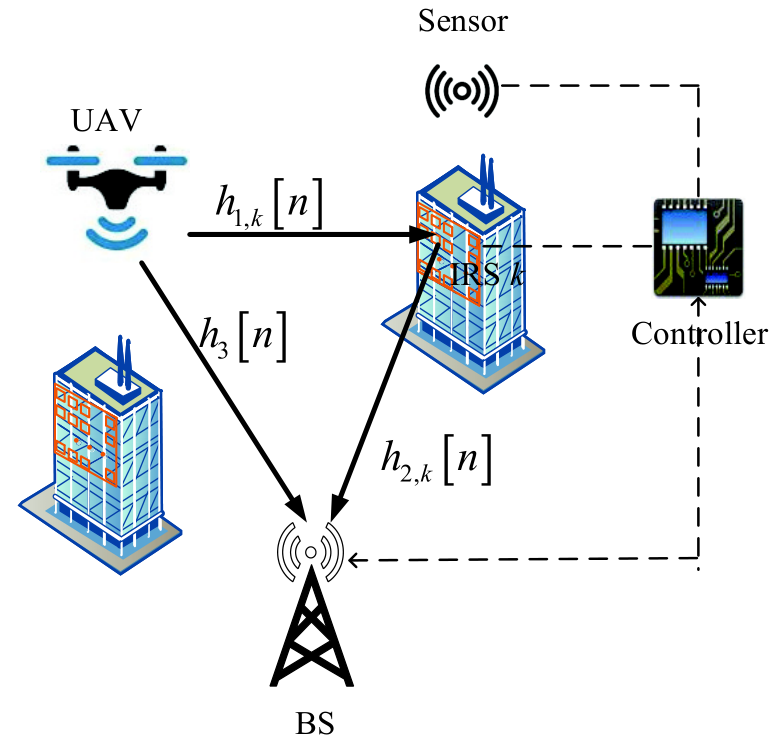
In this paper, we study an unmanned aerial vehicle (UAV)-assisted IRS symbiotic radio system, where the UAV is leveraged to assist the IRS data transmission. Specifically, we consider an urban environment, where there are multiple IRSs available to sense environmental information. As shown in Fig. 1, the IRS sends its own data to the BS by controlling its on/off state, and the receiver side (BS) uses the difference in channel response caused by the on/off state to decode the IRS information. The IRS also simultaneously tunes each reflecting element to align the phase of the signal passing through the UAV-IRS-BS link with that of the UAV-BS link to achieve coherent signal combining at the BS, thereby enhancing the UAV communication performance. In addition, the UAV’s flexible mobility can be exploited to create favorable channel conditions for the UAV-BS and UAV-IRS links. Our goal in this paper is to minimize the bit error rate (BER) of IRS by jointly optimizing the UAV trajectory, IRS phase shift matrix, and IRS scheduling, subject to a minimum data rate requirement for the UAV. We study two optimization objectives, one based on fairness for the IRS and the other on the weighted sum BER of the IRS. Then, we develop two novel algorithms to solve them. The main contributions of this paper are summarized as follows:
- •
We first consider the IRS weighted sum BER optimization problem, which is a mixed-integer and non-convex problem. To develop a low complexity algorithm, we propose a relaxation-based method. Specifically, we first relax the binary scheduling variables to continuous variables, and then we develop an alternating optimization (AO) algorithm to solve the relaxed non-convex optimization problem. We prove that the obtained scheduling results are the same as the binary results from the AO method, which means that no reconstruct strategy is needed, and thus the primary rate requirements of UAV are always satisfied. Numerical results show the proposed relaxation-based method converges within only a few iterations.
- •
We then take into account the fairness among multiple IRSs, and formulate a fairness BER optimization problem. The resultant problem is also a mixed integer and non-convex problem, which is in general difficult to solve optimally. We show that the commonly used relaxation-based method cannot be applied to this problem since the UAV’s rate requirement constraints may not be satisfied by the binary reconstruction operation for scheduling. To address this issue, a novel penalty-based algorithm is proposed. We first transform the binary constraints into a series of equivalent equality constraints, and then propose a two-layer algorithm to solve the problem. Numerical results show the effectiveness of this penalty-based algorithm.
- •
We conduct simulation results for the two proposed scenarios to illustrate their performance. For the first scenario, we study the impact of weighting factors on the system performance, and find that the optimized UAV trajectory places it closest to IRS with a high weighting factor. For the second scenario, the results show that the average fairness utility value is highly related to the IRS phase shift matrix. In addition, for both scenarios, the system performance is significantly improved by the optimized UAV trajectory as well as the finely tunable IRS phase shift.
The rest of this paper is organized as follows: Section II introduces the system model and problem formulation. In Sections III and IV, we study the weighted sum BER and fairness BER optimization problems, respectively. Numerical results are provided in Section V, and the paper is concluded in Section VI.
Notations: Boldface lower-case variables denote vectors. The notation represents the Euclidean norm of , the circularly symmetric complex Gaussian variable with mean and variance is denoted by , statistical expectation is defined as , statistical variance is defined as , and denotes the big-O computational complexity notation.
II System Model and Problem Formulation
II-A System Model
Consider a UAV-assisted IRS symbiotic radio system consisting of a single-antenna BS, a single-antenna UAV, and IRSs as shown in Fig. 1, where the UAV acts to help the IRS transmit its own data to the BS11 1 For ease of exposition, we term the UAV and BS as a primary network to assist the IRS’s information transmission.. The BS and IRS are in fixed locations, and the UAV can freely adjust its heading as it moves. The horizontal coordinates of the BS and the th IRS are respectively denoted as and . In addition, the altitude of the BS is denoted as , and the altitudes of all the IRSs are the same denoted as 22 2 Note that adopting different altitudes of IRSs do not affect the algorithm design in this paper.. We assume that the UAV flies in a periodic trajectory at a fixed altitude and with a given period . To make the problem tractable, the period is equally divided into time slots of duration . As a result, the trajectory of the UAV can be approximated by the two-dimensional sequences . Note that the duration should be chosen to be sufficiently small to satisfy , where denotes the maximum UAV speed, so that the UAV’s location can be considered as approximately unchanged within each time slot. The UAV mobility constraints are given below:
| (1) | ||||
| (2) |
where and represent the UAV’s initial and final location, respectively.
It is assumed that the IRS has reflecting elements, and the reflection coefficient matrix of IRS at time slot is defined by the diagonal matrix , where denotes the phase shift corresponding to the th reflecting element of IRS at time slot [11], [22],[29],[30]. Let , , and respectively denote the complex equivalent baseband channel vector between the UAV and the th IRS, between the th IRS and the BS, and between the UAV and the BS, at time slot , . To capture both the large-scale and small-scale fading, we model all channels as Rician [31]. Specifically, the channel coefficient between the UAV and IRS at time slot is given by [32]
| (3) |
where represents the large-scale fading channel coefficient, and denote the deterministic line-of-sight (LoS) channel component and the small-scale fading component, respectively, and is the Rician factor. The value of is related to the communication distance, and is given by
| (4) |
where denotes the channel power at the reference distance of meter, is the distance between the UAV and IRS , and denotes the path loss exponent. We assume that the IRS employs a uniform linear array (ULA) of reflecting elements, and thus is given by [32]
| (5) |
where denotes the IRS element spacing, denotes the carrier wavelength, and is the cosine of the angle of arrival (AoA) [33],[34]. The elements of of the non-LoS component are assumed to be independent and identically distributed and follow circularly symmetric complex Gaussian distribution with zero mean and unit variance.
Similarly, the channel vector between IRS and the BS at time slot is expressed as
| (6) |
where , , represents the path loss exponent, and is the corresponding Rician factor. , where denotes the cosine of the angle of departure (AoD). The elements of are also assumed to be independent and identically distributed and follow circularly symmetric complex Gaussian distribution with zero mean and unit variance.
Finally, for the UAV-BS link at time slot we have
| (7) |
where , , , path-loss exponent , and Rician factor . In addition, .
Remark 1: Although in this paper we adopt the ULA at IRS to facilitate the purpose of exposition, all the proposed algorithms are applicable to the case of uniform planar array (UPA) adopted at IRS with only a slight modifications for optimizing IRS phase shift discussed in (27) in Section III.
Remark 2: Generally, there are two main approaches for the IRS-involved channel acquisition, depending on whether the IRS elements are equipped with receive radio frequency (RF) chains or not [5]. For the first approach with active receive RF chains, conventional channel estimation methods can be applied for the IRS to estimate the channels of the UAV-IRS and IRS-BS links, respectively. In contrast, for the second approach without receive RF chains at the IRS, the IRS reflection patterns can be designed jointly with the uplink pilots to estimate the concatenated UAV-IRS-BS channel and UAV-BS channel e.g., [35], [36].
Typically, the symbol rate for the IRS transmission is much lower than that for the primary (UAV) transmission due to the limited computational and communication capabilities at the IRS. To describe it clearly, the frame structure for the IRS symbol, primary symbol, and channel coherence time is shown in Fig. 2. We assume that the duration of each UAV time slot equals the channel coherence time, i.e, . In the figure, represents the th IRS symbol transmitted to the BS in the th block of time slot , and is the primary symbol transmitted from the UAV to the BS at the th sub-block of block within time slot . Denote by and the durations of each IRS symbol and primary symbol, respectively. Without loss of generality, we assume that each IRS symbol covers primary symbols, namely , where is an integer, and . In addition, we assume , where is an integer, and .
To facilitate the system design, we consider a widely used wake-up communication scheduling approach [37],[38], where the UAV can only communicate with at most one IRS33 3 Strictly speaking, the UAV directly communicates with the controller at IRS rather than IRS itself. In the sequel, we will use the two terminologies interchangeably. at any time slot . Define the scheduling variable , where indicates that IRS is served by the UAV, and otherwise. We then have the following scheduling constraints
| (8) | ||||
| (9) |
If IRS is communicating with the UAV in time slot , the signal received by the BS at the th sub-block of block within time slot is given by
| (10) |
where denotes the transmit power at the UAV, , denotes the noise at IRS with power . We adopt the simple but widely used on-off keying (OOK) modulation for IRS’s information transmission, i.e., .
Since the IRS’s own signal and UAV’s primary signal are simultaneously received by the BS, to detect the composite signals correctly, several detectors such as maximum-likelihood (ML) detector, linear detector, and successive interference cancellation (SIC)-based detector, can be applied [39]. Furthermore, the strength of the signal received from UAV is generally much larger than that received from the IRS due to the following two reasons. First, the direct link between the UAV and the BS is always dominated by LoS due to the less scatters in the sky. Second, since the IRS consists of a large number of reflecting elements, it would significantly enhances the UAV’s signal transmission via adjusting the phase shifters. In addition, the SIC receiver decodes the stronger signal first, subtracts it from the composite signal, and extracts the weaker one from the residue. Therefore, the SIC based detector is practically appealing and applied in this paper [39], [40].
Define . It can be observed that contains , which changes relatively fast as compared to the channel variation. In other words, the IRS’s reflected signal plays the role of fast-varying channel components, making channel vary over the primary signal shown in (10). According to [26], [[32], Appendix B.7], [41], the achievable rate (bps/Hz) for the primary (UAV) system assisted by IRS is given by
| (11) |
where holds since under a channel coherence time, , , and are all invariant, while varies with the IRS’s reflected signal . Equality holds since we assume that the probability for sending symbol “1” at IRS is , and that for sending symbol “0” at IRS is , . It can be seen that the primary rate for each sub-block within time slot is the same. Thus, the achievable rate for the primary system assisted by IRS at time slot is given by .
After correctly decoding the primary signal , subtracting the primary signal from the composite signal, and we can obtain the intermediate signal as [40]
| (12) |
For the different IRS reflected symbols, the signals received at the BS have different amplitude values as
It is not difficult to check that44 4 Note that although is known at the BS after decoding, still can be regarded as a random variable following circularly symmetric complex Gaussian distribution during each one IRS symbol since each IRS symbol covers primary symbols.
We adopt a simple joint-energy detector for detecting IRS’s symbols [42], [43]. Define . It can be readily checked that a random variable is the sum of independent identically distributed central chi-squared random variables with two degrees of freedom. Suppose that the symbol “1” hypothesis is and symbol “0” hypothesis is , we can readily obtain the expectation and variance of as
| (17) |
with and . Based on the central limit theorem, when is large, the distribution of asymptotically approaches a Gaussian distribution as
| (18) |
Define probability density function . Following from [44], the decision criteria is if
| (19) |
then symbol “1” is chosen, otherwise, symbol “0” is chosen. As such, the BER of IRS can be derived from
| (20) |
where denotes the decision threshold. The optimal decision threshold can be derived by taking the first derivative of with respect to (w.r.t.) , which is given by
| (21) |
Therefore, the BER for detecting IRS ’s reflected symbol can be derived as
| (22) |
with the function given by . holds since for a large value , given in (21) approaches . We can see that the BER of IRS within each sub-block of time slot is the same. Thus, the BER for IRS at time slot is given by .
In this paper, we are interested in the average communication throughput and average BER. Theorem 1: The average achievable rate for the primary system, i.e., , is upper bounded by
| (23) |
where .
Proof: Please refer to Appendix A.
In Theorem 1, we can see that is determined by the deterministic LoS channel components , the large-scale fading coefficients , and the IRS phase shift matrix . It is worth pointing out that the above approximation will be tight if the SNR is sufficiently high [45].
Define SNR . Similarly, we can obtain the average SNR for IRS at time slot as
| (24) |
where .
II-B Problem Formulation
For the first scenario, our goal is to minimize the weighted sum BER among all IRSs over all the time slots by jointly optimizing the UAV trajectory, IRS phase shift matrix, and IRS scheduling. Accordingly, the problem can be formulated as
| (25a) | ||||
| (25b) | ||||
| (25c) | ||||
| (25d) | ||||
where denotes the weighting factor for IRS , with a higher value representing a higher priority over other IRSs, and is the minimum rate requirement of the primary transmission system for any time slot . Problem (25) is challenging to solve mainly due to the following three reasons. First, the optimization variables for communication scheduling are binary and thus (9), (25a), and (25b) involve integer constraints. Second, the IRS phase shift matrix, UAV trajectory, and IRS scheduling are intricately coupled in (25a) and (25b), which makes the problem non-convex. Third, the expression of in the objective function is implicit w.r.t. the optimization variables. In general, there is no efficient method to optimally solve problem (25).
For the second scenario, our goal is to minimize the maximum BER among all IRS over all the time slots by jointly optimizing the UAV trajectory, the IRS phase shift matrix, and the IRS scheduling. Accordingly, the problem can be formulated as
| (26a) | ||||
| (26b) | ||||
| (26c) | ||||
| (26d) | ||||
The left hand side of (26b) denotes the average BER of IRS over all time slots. Problem (26) is still difficult to solve due to the similar challenges for the weighted sum BER problem discussed above.
Remark 3: It can be seen that given in (22) is a complicated expression with an integral, which is challenging to analyze directly. In addition, it can be readily verified that function is monotonically decreasing with SNR . Instead of maximizing the SNR directly, we introduce a utility function , which is a differential, concave and monotonically increasing function w.r.t. , to replace BER . In addition, to obtain the average BER , we set the upper bound of , i.e., , as our design metric for facilitating the algorithm design. In the subsequent sections, instead of minimizing the BER directly, we aim to maximize the corresponding utility functions.
III Relaxation-based Algorithm for Weighted Sum BER Optimization Problem
In this section, we propose a relaxation-based algorithm to solve problem (25). Specifically, we first relax the binary scheduling variables into continuous variables, and divide the relaxed non-convex problem into two sub-problems, then solve these two sub-problems. However, even with this decomposition, the problem is still difficult to handle due to the non-convex cosine in both the objective function and constraints. To address this issue, we first obtain a closed-form solution for the IRS phase shift matrix for a given UAV trajectory and communication scheduling, and then substitute this expression into the original problem resulting in a joint IRS scheduling and UAV trajectory optimization problem. We first develop the following theorem:
Theorem 2: For any given UAV trajectory and IRS scheduling, the optimal IRS phase shift matrix that maximizes the primary rate and SNR is given by
| (27) |
Proof: Please refer to Appendix B.
From Appendix B, we can see that the maximizer of the terms and are respectively given by
| (28) |
and
| (29) |
Substituting (28) and (29) in (23) and (24), respectively, we have
| (30) |
and
| (31) |
where , , and .
As a result, the weighted sum BER optimization problem (25) can be simplified as
| (32a) | ||||
| (32b) | ||||
| (32c) | ||||
It can be seen that (32) only involves two variables, and , and the cosine function no longer appears, which thus make the problem easier to solve. In the following, a low complexity algorithm based on the relaxation method is proposed. Note that different from [38],[46],[47], where the resulting continuous scheduling variables need to be converted into binary. However, for problem (32), we prove that the converged relaxation scheduling variables are binary, which means that no reconstruct strategy is needed, and thus the UAV rate constraints (32b) are automatically satisfied. Specifically, we first relax the binary variable to a continuous variable, and rewrite constraint (9) as follows [38],[46],[47]:
| (33) |
We then decompose the relaxed problem into two separate subproblems, IRS scheduling and UAV trajectory optimization, and then alternately optimize each one.
III-A IRS Scheduling Optimization
For any given UAV trajectory , the IRS scheduling problem of (32) becomes
| (34a) | ||||
| (34b) | ||||
Since both the objective function and constraints are linear w.r.t. , problem (34) is thus a linear optimization problem.
Theorem 3: The optimal solution to problem (34) is binary, i.e., .
Proof: Please refer to Appendix C.
Theorem 3 shows that even though the binary constraint in the IRS scheduling problem of (34) has been relaxed, the obtained solution is still a binary result. As such, no reconstruction operation is needed. In addition, since (34) is a linear optimization problem, it has very low computational complexity [48].
III-B UAV Trajectory Optimization
For any given IRS scheduling , the UAV trajectory optimization problem of (32) becomes
| (35a) | ||||
| (35b) | ||||
Note that (35) is neither concave or quasi-concave due to the non-convex constraints (32b) and non-convex objective function (35a). In general, there is no efficient method to obtain the optimal solution. In the following, we adopt the successive convex optimization technique to solve (35). To this end, we introduce additional slack variables and , and recast (35) as
| (36a) | ||||
| (36b) | ||||
| (36c) | ||||
| (36d) | ||||
| (36e) | ||||
It can be shown that at the optimal solution to (36), we must have and , since otherwise we can always increase (or ) without decreasing the value of the objective. Therefore, problem (36) is equivalent to problem (35). With this reformulation, objective function (36a) is now concave w.r.t. , but with the new non-convex constraints (36c) and (36d). The key observation is that in (36c), although , defined in (4), is not convex w.r.t. , it is convex w.r.t. . Recall that any convex function is globally lower-bounded by its first-order Taylor expansion at any feasible point [49]. Therefore, for any local point obtained at the th iteration, we have
| (37) |
Define the new constraint as
| (38) |
which is convex since is a quadratic function w.r.t. . Similarly, for any local point obtained at the th iteration, with and
In addition, to tackle the non-convexity of constraint (36b), we introduce variable , and reformulate (36b) as
| (40) |
with the additional constraint
| (41) |
Both constraints (40) and (41) are convex since we can see that the left hand side of (40) is a log function, which is concave, and the right hand side of (41) is a quadratic-over-linear fractional function, which is convex. As a result, for any given local points and , we have the following optimization problem
| (42a) | ||||
| (42b) | ||||
III-C Convergence Analysis and Computational Complexity
In the proposed AO algorithm, we solve the relaxed problem (32) by iteratively solving problems (34) and (42), where the solution obtained for one subproblem in each iteration is used as the initial point for the other. The detailed procedure for solving (32) is summarized in Algorithm 1. The convergence of Algorithm 1 has been well studied in [50], and is omitted here for brevity.
We now analyze the complexity of Algorithm 1. In step 4, (34) is a linear optimization problem whose complexity is [48], where denotes the number of variables. In step 5, the complexity for solving (42) by the interior point method is [51], where denotes the number of variables. Therefore, the total complexity of Algorithm 1 is , where stands for the number of iterations required to reach convergence.
IV Penalty-based Algorithm for Fairness BER Optimization Problem
In this section, we aim to solve problem (26). Based on Theorem 2, (30), and (31) in Section III, problem (26) is simplified as
| (43a) | ||||
| (43b) | ||||
| (43c) | ||||
| (43d) | ||||
Unfortunately, the low-complexity algorithm based on the relaxation-based method cannot be applied to problem (43) due to the primary rate requirement (43c). More specifically, when converting the continuous-valued solutions for the obtained by the relaxed problem to binary, e.g., using the rounding function [46], constraint (43c) will in general no longer be satisfied. In this section, we propose a two-layer penalty-based algorithm to solve (43). The inner layer solves a penalized optimization problem by applying the AO method, while the outer layer updates the penalty coefficient, until convergence is achieved. Specifically, in the inner layer, the original problem (43) is decomposed into three subproblems: IRS phase shift matrix optimization, IRS scheduling optimization, and UAV trajectory optimization.
We first introduce slack variables to transform the binary constraints into a series of equivalent equality constraints. Specifically, (9) can be rewritten as
| (44) |
| (45) |
From (44) and (45), we can readily derive that the that satisfies the above two constraints must be either or , which confirms the equivalence of the transformation of (9) into the two constraints. We then use (44) and (45) in a penalty term that is added to the objective function of (43), yielding the following optimization problem
| (46a) | ||||
| (46b) | ||||
where is the penalty coefficient used to penalize the violation of the equality constraints (44) and (45) [50]. While these equality constraints become satisfied as , it is not effective to initially set to be a very small value since in this case the objective will be dominated by the penalty terms, and the term will be diminished. In contrast, initializing with a larger value allows us to obtain a good starting point for the proposed algorithm. Then, by gradually decreasing the value of , we can finally obtain a solution that satisfies (44) and (45) within a predefined accuracy. Note that, for any given penalty coefficient , problem (46) is still non-convex due to the non-convex constraints (43b) and (43c). We then apply the AO method to iteratively optimize the primary variables in different blocks [50]. Specifically, in the inner layer, problem (46) is divided into three subproblems in which , , and are optimized iteratively as follows:
IV-A Inner layer iteration
1) Optimizing for given and . This subproblem can be expressed as
| (47a) | ||||
| (47b) | ||||
We can see that only the auxiliary variable is involved in the objective function. Therefore, setting the derivative of (47) w.r.t. to zero, the solution can be obtained as
| (48) |
2) Optimizing for given and . This subproblem is written as
| (49a) | ||||
| (49b) | ||||
It can be seen that (49) is convex with a quadratic objective function and linear inequality constraints, which can be numerically solved by standard convex optimization techniques, such as the interior-point method [49].
3) Optimizing for given and . Ignoring the constant terms that are irrelevant to the UAV trajectory, this subproblem is formulated as:
| (50a) | ||||
| (50b) | ||||
Note that (50) is neither concave or quasi-concave due to the non-convex constraints (43b) and (43c). In general, there is no efficient method to obtain the optimal solution. In the following, we adopt the successive convex optimization technique to solve (50). Using the previous analysis of the UAV trajectory optimization for problem (35) in Section III-B, by introducing the same slack variables and local points and , we can directly derive the following equivalent convex optimization problem
IV-B Outer layer iteration
In the outer layer, we gradually decrease the value of the penalty coefficient as follow
| (52) |
where is a scaling factor, where a larger value of can achieve better performance but at the cost of more iterations in the outer layer.
IV-C Convergence Analysis and Computational Complexity
To show the converged solutions of the proposed penalty-based algorithm, the terminal criteria for the outer layer is given as follows;
| (53) |
where is a predefined accuracy. The detailed procedure of the penalty-based algorithm is summarized in Algorithm 2.
In the inner layer, with the given penalty coefficient, the objective function of (46) is non-increasing over each iteration after applying the AO method, and the objective of (46) is bounded due to the limited flying time and transmit power . As such, a stationary point can be achieved in the inner layer. In the outer layer, we gradually decrease the penalty coefficient so that the equality constraints (44) and (45) are ultimately satisfied. Based on the results in [52, Appendix B], this penalty-based framework is guaranteed to converge.
The complexity of Algorithm 2 can be quantified as follows. In the inner layer, the main complexity of Algorithm 2 comes from steps 5 and 6. In step 5, the complexity of computing is [51], where stands for the number of variables [53]. Similarly, in step 6, the complexity required to compute the UAV trajectory is [51], where denotes the number of variables. Therefore, the total complexity of Algorithm 2 is , where and respectively denote the number of iterations required for reaching convergence in the inner layer and outer layer.
V Numerical Results
In this section, we provide numerical results to verify the performance of the proposed algorithm for the UAV assisted IRS symbiotic radio transmission system. In the simulation, we consider a system that operates on a carrier frequency of with the system bandwidth of and the effective noise power density . As such, the noise power at the BS and the channel gain are set to and , respectively [54]. In addition, we set [55]. The UAV altitude is fixed at with transmit power and maximum speed . The UAV’s initial and final location are set to . The altitudes of the BS and IRS are both set to . The duration of each time slot is . The path loss exponents for the UAV-IRS link, IRS-BS link, and UAV-BS link are assumed to be the same , and the Rician factors for the above links are set to be . Without loss of generality, we set the utility function as a logarithm function with base , which naturally achieves a certain of fairness among the information transmission of multiple IRSs, and has been widely adopted in the literature, such as [56]. Unless otherwise specified, we set , , , , , .
V-A Weighted Sum BER Optimization
This subsection evaluates the performance of Algorithm 1 for the weighted sum BER problem (25). We consider IRS, which are located at in a horizontal plane. Unless otherwise specified, the weighting factors are set as . To show the efficiency of Algorithm 1, its convergence behaviour for the two different periods is plotted in Fig. 4. It is observed that the average weighted sum utility value increases quickly with the number of iterations, and in both cases converges within only iterations.
In Fig. 4, the optimized UAV trajectories obtained by Algorithm 1 when are studied for two different weighting factors, i.e., and . We see that the UAV sequentially visits all IRS for the weighting factor , since the path loss between the UAV and IRS is significantly reduced when the UAV is nearby, thereby improving the utility value. However, for weighting factor , the UAV only does a close fly-by of IRS 3 rather than hovering above it, since places a lower weight on IRS 3 and hence reduces its priority relative to the others. To see this more clearly, in Fig. 6 the UAV speed profile for the two weighting factors is plotted. Compared with , for the UAV spends less time hovering above IRS for serving.
In Fig. 6, the IRS scheduling for is plotted. We see that for optimizing the weighted sum utility, the IRSs are scheduled for different lengths of time as shown in Fig. 6. As before, the IRS scheduling results are indeed binary, which verifies the effectiveness of Algorithm 1.
In Fig. 8, we compares the average weighted sum utility value versus achieved by the following schemes: 1) Proposed scheme in Algorithm 1; 2) Circular trajectory, where the UAV flies with a circle path of radius (corresponding to the distance from the BS to the UAV’s initial/final location) and center ; 3) Fixed phase shifts, where the IRS phase shifts for all the elements is fixed at either or . For the fixed phase shift examples, the UAV trajectory is set to be the result obtained by the proposed scheme. The upper bound for the weighted sum BER problem is given by the solution to
| (54) |
It is observed from Fig. 8 that our proposed algorithm substantially outperforms the other methods in terms of average weighted sum utility value. This is expected since an optimized UAV trajectory can establish better channel conditions for the IRS, which significantly increases IRS’s SNR. In addition, by adjusting the IRS phase shifts to align the cascaded AoA and AoD with the UAV-BS link, i.e., as shown in Theorem 2, the SNR of the UAV-IRS-BS link will be significantly increased.
In Fig. 8, we study the average weighted sum utility value versus the number of IRS reflecting elements . The performance gain of the proposed approach and the circular trajectory increases with , since more reflecting elements help achieve higher passive beamforming gain. In addition, our proposed approach outperforms the circular trajectory by leveraging the UAV mobility. Clearly, the IRS has a significant impact on the system performance, and the IRS phase shifts must be finely tuned in the system design.
V-B Fairness BER Optimization
This subsection evaluates the performance of Algorithm 2 for the fairness BER problem (26). The initial setup for the fairness BER problem simulations are the same as those used for evaluating the weighted sum BER approach discussed above. Fig. 9 shows the penalty violation in (53) and the convergence behavior of Algorithm 2 under different periods . It can be seen from Fig. 9(a) that converges very fast with the value decreasing to after iterations for . Even when , the constraint is eventually satisfied within the predefined accuracy (i.e., ) by iterations, which indicates that the proposed penalty-based algorithm can effectively tackle the binary scheduling constraints. In addition, in Fig. 9(b), we plot the fairness utility value versus the number of outer layer iterations. We see that the fairness utility value increases quickly with the number of outer layer iterations for both the and cases, and convergence to a fraction of the final value is achieved only 4 iterations.
In Fig. 11, the optimized trajectories obtained by Algorithm 2 for and are plotted. As increases, the UAV exploits its mobility to adaptively enlarge and adjust its trajectory to move closer to each IRS. When becomes sufficiently large, i.e., , the UAV is able to sequentially visit all the IRS and stay stationary above each of them for a certain amount of time. This is expected since when the distance between the UAV and IRS is small, the length of the double channel fading propagation, i.e., the UAV-IRS-BS link, will be reduced, thus improving the IRS transmission SNR. To see this more clearly, Fig. 11 plots the UAV speed for the case when . We see that the UAV flies either with maximum or zero speed, indicating that the UAV flies with maximum UAV speed to move closer to the IRS, and then remains stationary above it as soon as possible. Additionally, we observe in Fig. 13 that the IRS sequentially communicates with each UAV to experience better channel conditions, and the scheduling results are indeed binary, which demonstrates that the constraints in (44) and (45) are satisfied by the proposed Algorithm 2.
In Fig. 13, we study the average fairness utility value versus period for our proposed scheme compared with the same benchmarks as those considered for the weighted sum BER problem in Fig. 8. Fig. 13 shows that the fairness utility value for the circular trajectory is constant regardless of the period due to the time-invariant air-to-ground channels. In contrast, the fairness utility value achieved by the proposed scheme increases with , which further demonstrates the benefits of leveraging the UAV mobility. The calculation of the upper bound for the fairness BER problem is different from that for the weighted sum BER problem. When is sufficiently large, it can be assumed that the amount of time each IRS served is equal. As for the case when the UAV hovers above the IRS, an upper bound for the fairness BER problem can be obtained by solving the following problem
| (55a) | ||||
| (55b) | ||||
| (55c) | ||||
where the term represents the achievable rate for the IRS when the UAV is directly above IRS , and denotes the travel time ratio for IRS . Problem (55) is a linear optimization problem, and thus can be easily solved by the interior point method.
In Fig. 14, the average fairness utility value versus the number of IRS reflecting elements is studied. We see that the performance gain of the proposed scheme increases as the number of IRS reflecting elements increases, since more reflecting elements help achieve higher passive beamforming gain. In addition, the performance of the fixed IRS phase shift scheme is very poor, and the average fairness utility value nearly approaches zero due to the unaligned angles of the UAB-IRS-BS and UAV-BS links, which implies that the IRS phase shift must be carefully tuned.
VI Conclusion
In this paper, we studied a UAV-assisted IRS symbiotic radio system. We exploited the UAV mobility to maximize the data information transferred from several IRSs to a given BS. We first studied a weighted sum BER minimization problem by jointly optimizing the UAV trajectory, IRS phase shifts, and IRS scheduling, and proposed a low-complexity relaxation-based method to solve it. We proved that the solution to the relaxed problem provides binary scheduling results, and hence no additional operation is needed to enforce this constraint. We then considered fairness among the IRSs, and developed a fairness BER optimization problem. To handle the resulting mixed integer non-convex problem, we transformed the binary constraints into an equivalent set of equality constraints, and proposed a penalty-based method to address the constraints. The effectiveness of this approach was justified by the numerical simulations. Simulation results demonstrated that the system performance can be significantly improved by optimizing the UAV trajectory as well as the IRS phase shifts.
Appendix A Proof of Theorem 1
To show Theorem 1, we first define the function . It can be readily checked that is concave with respect to . Thus, based on Jensen’s inequality [49], we have . Therefore, the following inequality holds
| (56) |
Since the small-scale fading channel coefficients , , and are independent of each other, we can obtain
| (57) |
where ,
, ,
, and
. We first calculate
| (58) |
where holds since , , and
. We can obtain the remaining terms as follows:
| (59) |
In addition, we have . Combining all of the above results, we can directly arrive at (23).
Appendix B Proof of Theorem 2
Here we derive a closed-form solution for the IRS phase shifts that maximize the primary rate expression in (23). We have the following inequality
| (60) |
where is due to the triangle inequality, which holds with equality if and only if , . This indicates that the th phase shift at IRS should be tuned such that the phase of the signal that passes through the UAV-IRS and IRS-BS links is aligned with that of the signal over the UAV-BS direct link to achieve coherent signal combining at the BS. Thus, we can obtain the closed-form IRS phase shift expression in (27). In addition, it can be easily checked that in (27) is also the optimal solution that maximizes the IRS reflecting rate in (24). This completes the proof of Theorem 2.
Appendix C Proof of Theorem 3
It can be readily verified that problem (34) satisfies Slater’s condition, and thus strong duality holds and its optimal solution can be obtained by solving its dual problem [49]. Specifically, we first introduce the dual variables associated with the primary rate constraints (32b), and derive the partial Lagrangian of problem (34) as follows
| (61) |
The Lagrange dual function of (34) is defined as
| (62a) | ||||
| (62b) | ||||
It can be seen that the dual function (62) can be divided into subproblems that can be solved in parallel. The -th subproblem of (62) can be written as
| (63a) | ||||
| (63b) | ||||
| (63c) | ||||
It can be easily derived that the optimal solution that maximizes (63) is either or for , where subscript corresponds to the index that maximizes among all . This also holds for the case that there are more than two IRS that have the same maximum value of among all . This thus completes the proof of Theorem 3.
References
- [1] Q. Wu, G. Y. Li, W. Chen, D. W. K. Ng, and R. Schober, “An overview of sustainable green 5G networks,” IEEE Wireless Commun., vol. 24, no. 4, pp. 72–80, Aug. 2017.
- [2] A. L. Swindlehurst, E. Ayanoglu, P. Heydari, and F. Capolino, “Millimeter-wave massive MIMO: The next wireless revolution?” IEEE Commun. Mag., vol. 52, no. 9, pp. 56–62, Sept. 2014.
- [3] M. Kamel, W. Hamouda, and A. Youssef, “Ultra-dense networks: A survey,” IEEE Commun. Surveys Tuts., vol. 18, no. 4, pp. 2522–2545, 4th Quat. 2016.
- [4] L. Lu, G. Y. Li, A. L. Swindlehurst, A. Ashikhmin, and R. Zhang, “An overview of massive MIMO: Benefits and challenges,” IEEE J. Sel. Top. Sign. Proces., vol. 8, no. 5, pp. 742–758, Oct. 2014.
- [5] Q. Wu and R. Zhang, “Towards smart and reconfigurable environment: Intelligent reflecting surface aided wireless network,” IEEE Commun. Mag., vol. 58, no. 1, pp. 106–112, Jan. 2020.
- [6] T. J. Cui, S. Liu, and L. Zhang, “Information metamaterials and metasurfaces,” J. Phys. Chem. C, vol. 5, no. 15, pp. 3644–3668, 2017.
- [7] W. Tang, M. Z. Chen, X. Chen, J. Y. Dai, Y. Han, M. Di Renzo, Y. Zeng, S. Jin, Q. Cheng, and T. J. Cui, “Wireless communications with reconfigurable intelligent surface: Path loss modeling and experimental measurement,” IEEE Trans. Wireless Commun., 2020, early access, doi: 10.1109/TWC.2020.3024887.
- [8] C. Liaskos, S. Nie, A. Tsioliaridou, A. Pitsillides, S. Ioannidis, and I. Akyildiz, “A new wireless communication paradigm through software-controlled metasurfaces,” IEEE Commun. Mag., vol. 56, no. 9, pp. 162–169, 2018.
- [9] M. Di Renzo, M. Debbah, D.-T. Phan-Huy, A. Zappone, M.-S. Alouini, C. Yuen, V. Sciancalepore, G. C. Alexandropoulos, J. Hoydis, H. Gacanin et al., “Smart radio environments empowered by reconfigurable AI meta-surfaces: An idea whose time has come,” EURASIP J. Wireless Commun. Netw., vol. 2019, no. 1, pp. 1–20, May 2019.
- [10] Q. Wu, S. Zhang, B. Zheng, C. You, and R. Zhang, “Intelligent reflecting surface aided wireless communications: A tutorial,” IEEE Trans. Commun., to appear, 2020. [Online]. Available: https://arxiv.org/abs/2007.02759v2.
- [11] Q. Wu and R. Zhang, “Intelligent reflecting surface enhanced wireless network via joint active and passive beamforming,” IEEE Trans. Wireless Commun., vol. 18, no. 11, pp. 5394–5409, Nov. 2019.
- [12] C. Huang, R. Mo, and C. Yuen, “Reconfigurable intelligent surface assisted multiuser MISO systems exploiting deep reinforcement learning,” IEEE J. Sel. Areas Commun., vol. 38, no. 8, pp. 1839–1850, Aug. 2020.
- [13] C. Pan, H. Ren, K. Wang, W. Xu, M. Elkashlan, A. Nallanathan, and L. Hanzo, “Multicell MIMO communications relying on intelligent reflecting surface,” IEEE Trans. Wireless Commun., vol. 19, no. 8, pp. 5218–5233, Aug. 2020.
- [14] C. Huang, A. Zappone, G. C. Alexandropoulos, M. Debbah, and C. Yuen, “Reconfigurable intelligent surfaces for energy efficiency in wireless communication,” IEEE Trans. Wireless Commun., vol. 18, no. 8, pp. 4157–4170, 2019.
- [15] S. Zhang and R. Zhang, “Intelligent reflecting surface aided multiple access: Capacity region and deployment strategy,” 2020. [Online]. Available: https://arxiv.org/abs/2002.07091.
- [16] X. Guan, Q. Wu, and R. Zhang, “Joint power control and passive beamforming in IRS-assisted spectrum sharing,” IEEE Commun. Lett., vol. 24, no. 7, pp. 1553–1557, 2020.
- [17] H. Yang, Z. Xiong, J. Zhao, D. Niyato, L. Xiao, and Q. Wu, “Deep reinforcement learning based intelligent reflecting surface for secure wireless communications,” IEEE Trans. Wireless Commun., 2020, early access, doi: 10.1109/TWC.2020.3024860.
- [18] G. Zhou, C. Pan, H. Ren, K. Wang, and A. Nallanathan, “A framework of robust transmission design for IRS-aided MISO communications with imperfect cascaded channels,” IEEE Trans. Signal Process., vol. 68, pp. 5092–5106, 2020.
- [19] X. Lu, W. Yang, X. Guan, Q. Wu, and Y. Cai, “Robust and secure beamforming for intelligent reflecting surface aided mmwave MISO systems,” IEEE Wireless Commun. Lett., vol. 9, no. 12, pp. 2068–2072, Dec. 2020.
- [20] Y. Yang, B. Zheng, S. Zhang, and R. Zhang, “Intelligent reflecting surface meets OFDM: Protocol design and rate maximization,” IEEE Trans. Commun., vol. 68, no. 7, pp. 4522–4535, Jul. 2020.
- [21] Y. Yang, S. Zhang, and R. Zhang, “IRS-enhanced OFDMA: Joint resource allocation and passive beamforming optimization,” IEEE Wireless Commun. Lett., vol. 9, no. 6, pp. 760–764, Jun. 2020.
- [22] Q. Wu and R. Zhang, “Weighted sum power maximization for intelligent reflecting surface aided SWIPT,” IEEE Wireless Commun. Lett., vol. 9, no. 5, pp. 586–590, May 2020.
- [23] C. Pan, H. Ren, K. Wang, M. Elkashlan, A. Nallanathan, J. Wang, and L. Hanzo, “Intelligent reflecting surface aided MIMO broadcasting for simultaneous wireless information and power transfer,” IEEE J. Sel. Areas Commun., vol. 38, no. 8, pp. 1719–1734, Aug. 2020.
- [24] Z. Li, W. Chen, and Q. Wu, “Joint beamforming design and power splitting optimization in IRS-assisted SWIPT NOMA networks,” 2020. [Online]. Available: https://arxiv.org/abs/2011.14778.
- [25] W. Yan, X. Yuan, and X. Kuai, “Passive beamforming and information transfer via large intelligent surface,” IEEE Wireless Communications Letters, vol. 9, no. 4, pp. 533–537, Apr. 2020.
- [26] Q. Zhang, Y. Liang, and H. V. Poor, “Large intelligent surface/antennas (LISA) assisted symbiotic radio for IoT communications,” 2020. [Online]. Available: https://arxiv.org/abs/2002.00340v1.
- [27] J. Hu, Y. C. Liang, and Y. Pei, “Reconfigurable intelligent surface enhanced multi-user MISO symbiotic radio system,” IEEE Trans. Commun., 2020, early access, doi=10.1109/TCOMM.2020.3047444.
- [28] R. Y. Mesleh, H. Haas, S. Sinanovic, C. W. Ahn, and S. Yun, “Spatial modulation,” IEEE Trans. Veh. Technol., vol. 57, no. 4, pp. 2228–2241, Jul. 2008.
- [29] G. Zhou, C. Pan, H. Ren, K. Wang, and A. Nallanathan, “Intelligent reflecting surface aided multigroup multicast MISO communication systems,” IEEE Trans. Signal Process., vol. 68, pp. 3236–3251, 2020.
- [30] S. Zhang and R. Zhang, “Capacity characterization for intelligent reflecting surface aided MIMO communication,” IEEE J. Sel. Areas Commun., vol. 38, no. 8, pp. 1823–1838, Aug. 2020.
- [31] C. Zhan and Y. Zeng, “Aerial-ground cost tradeoff for multi-UAV-enabled data collection in wireless sensor networks,” IEEE Trans. Commun., vol. 68, no. 3, pp. 1937–1950, Mar. 2020.
- [32] D. Tse and P. Viswanath, Fundamentals of Wireless Communication. Cambridge, U.K,: Cambridge Univ. Press, 2005.
- [33] S. Li, B. Duo, X. Yuan, Y. Liang, and M. Di Renzo, “Reconfigurable intelligent surface assisted UAV communication: Joint trajectory design and passive beamforming,” IEEE Wireless Commun. Lett., vol. 9, no. 5, pp. 716–720, May 2020.
- [34] H. Long, M. Chen, Z. Yang, B. Wang, Z. Li, X. Yun, and M. Shikh-Bahaei, “Reflections in the sky: Joint trajectory and passive beamforming design for secure UAV networks with reconfigurable intelligent surface,” 2020. [Online]. Available: https://arxiv.org/abs/2005.10559.
- [35] S. Lin, B. Zheng, G. C. Alexandropoulos, M. Wen, F. Chen, and S. sMumtaz, “Adaptive transmission for reconfigurable intelligent surface-assisted OFDM wireless communications,” IEEE J. Sel. Areas Commun., vol. 38, no. 11, pp. 2653–2665, 2020.
- [36] B. Zheng and R. Zhang, “Intelligent reflecting surface-enhanced OFDM: Channel estimation and reflection optimization,” IEEE Wireless Commun. Lett., vol. 9, no. 4, pp. 518–522, Apr. 2020.
- [37] M. Hua, Y. Wang, Q. Wu, H. Dai, Y. Huang, and L. Yang, “Energy-efficient cooperative secure transmission in multi-UAV-enabled wireless networks,” IEEE Trans. Veh. Technol., vol. 68, no. 8, pp. 7761–7775, Aug. 2019.
- [38] Q. Wu, Y. Zeng, and R. Zhang, “Joint trajectory and communication design for multi-UAV enabled wireless networks,” IEEE Trans. Wireless Commun., vol. 17, no. 3, pp. 2109–2121, Mar. 2018.
- [39] G. Yang, Q. Zhang, and Y.-C. Liang, “Cooperative ambient backscatter communications for green internet-of-things,” IEEE Internet of Things J., vol. 5, no. 2, pp. 1116–1130, 2018.
- [40] S. Verdu et al., Multiuser detection. Cambridge university press, 1998.
- [41] R. Long, Y. Liang, H. Guo, G. Yang, and R. Zhang, “Symbiotic radio: A new communication paradigm for passive internet of things,” IEEE Internet of Things J., vol. 7, no. 2, pp. 1350–1363, Feb. 2020.
- [42] J. Qian, F. Gao, G. Wang, S. Jin, and H. Zhu, “Noncoherent detections for ambient backscatter system,” IEEE Trans. Wireless Commun., vol. 16, no. 3, pp. 1412–1422, Mar. 2017.
- [43] M. Hua, L. Yang, C. Li, Z. Zhu, and I. Lee, “Bistatic backscatter communication: Shunt network design,” IEEE Internet of Things J., 2020, early access, doi: 10.1109/JIOT.2020.3040963.
- [44] S. M. Kay, Fundamentals of statistical signal processing. Prentice Hall PTR, 1993.
- [45] Y. Han, W. Tang, S. Jin, C. Wen, and X. Ma, “Large intelligent surface-assisted wireless communication exploiting statistical CSI,” IEEE Trans. Veh. Technol., vol. 68, no. 8, pp. 8238–8242, Aug. 2019.
- [46] M. Hua, L. Yang, C. Pan, and A. Nallanathan, “Throughput maximization for full-duplex UAV aided small cell wireless systems,” IEEE Wireless Commun. Lett., vol. 9, no. 4, pp. 475–479, Apr. 2020.
- [47] M. Hua, Y. Wang, Z. Zhang, C. Li, Y. Huang, and L. Yang, “Power-efficient communication in UAV-aided wireless sensor networks,” IEEE Commun. Lett., vol. 22, no. 6, pp. 1264–1267, Jun. 2018.
- [48] J. Gondzio and T. Terlaky, “A computational view of interior point methods,” Advances in linear and integer programming. Oxford Lecture Series in Mathematics and its Applications, vol. 4, pp. 103–144, 1996.
- [49] S. Boyd and L. Vandenberghe, Convex optimization. Cambridge university press, 2004.
- [50] D. P. Bertsekas, Nonlinear Programming. Athena Scientific, 1999.
- [51] G. Zhang, Q. Wu, M. Cui, and R. Zhang, “Securing UAV communications via joint trajectory and power control,” IEEE Trans. Wireless Commun., vol. 18, no. 2, pp. 1376–1389, Feb. 2019.
- [52] Y. Cai, Q. Shi, B. Champagne, and G. Y. Li, “Joint transceiver design for secure downlink communications over an amplify-and-forward MIMO relay,” IEEE Trans. Commun., vol. 65, no. 9, pp. 3691–3704, Sept. 2017.
- [53] S. Boyd, EE364b Convex Optimization. [Online]. Available: https://web.stanford.edu/class/ee364b/lectures.html
- [54] J. Xu, Y. Zeng, and R. Zhang, “UAV-enabled wireless power transfer: Trajectory design and energy optimization,” IEEE Trans. Wireless Commun., vol. 17, no. 8, pp. 5092–5106, Aug. 2018.
- [55] Q. Wu and R. Zhang, “Joint active and passive beamforming optimization for intelligent reflecting surface assisted SWIPT under QoS constraints,” IEEE J. Sel. Areas Commun., vol. 38, no. 8, pp. 1735–1748, Aug. 2020.
- [56] Q. Ye, B. Rong, Y. Chen, M. Al-Shalash, C. Caramanis, and J. G. Andrews, “User association for load balancing in heterogeneous cellular networks,” IEEE Trans. Wireless Commun., vol. 12, no. 6, pp. 2706–2716, Jun. 2013.