Diffusion Equations for Medical Images
In brain imaging, the image acquisition and processing processes themselves are likely to introduce noise to the images. It is therefore imperative to reduce the noise while preserving the geometric details of the anatomical structures for various applications. Traditionally Gaussian kernel smoothing has been often used in brain image processing and analysis. However, the direct application of Gaussian kernel smoothing tend to cause various numerical issues in irregular domains with boundaries. For example, if one uses large bandwidth in kernel smoothing in a cortical bounded region, the smoothing will blur signals across boundaries. So in kernel smoothing and regression literature, various ad-hoc procedures were introduce to remedy the boundary effect.
Motivated by Perona & Malik 1990, diffusion equations have been widely used in brain imaging as a form of noise reduction. The most natural straightforward way to smooth images in irregular domains with boundaries is to formulate the problem as boundary value problems using partial differential equations. Numerous diffusion-based techniques have been developed in image processing (Sochen et al. 1998; Malladi & Ravve 2002; Tang et al. 1999; Taubin 2000; Andrade et al. 2001; Chung et al. 2001; Chung, Worsley, Robbins, Paus, Taylor, Giedd, Rapoport & Evans 2003; Chung, Robbins & Evans 2005; Chung & Taylor 2004; Cachia, Mangin, Riviére, Papadopoulos-Orfanos, Kherif, Bloch & Régis 2003; Cachia, Mangin, Riviére, Kherif, Boddaert, Andrade, Papadopoulos-Orfanos, Poline, Bloch, Zilbovicius, Sonigo, Brunelle & Régis 2003; Joshi et al. 2009). In this paper, we will overview the basics of isotropic diffusion equations and explain how to solve them on regular grids and irregular grids such as graphs.
1 Diffusion as a Cauchy problem
Consider to be a compact differentiable manifold. Let be the space of square integrable functions in with inner product
| (1) |
where is the Lebegue measure such that is the total volume of . The norm is defined as
The linear partial differential operator is self-adjoint if
for all . Then the eigenvalues and eigenfunctions of the operator are obtained by solving
| (2) |
Often (2) is written as
so care should be taken in assigning the sign of eigenvalues.
Theorem 1.1
The eigenfunctions are orthonormal.
Proof. Note . On the other hand, . Thus
For any , , orthogonal. For to be orthonormal, we need . This is simply done by absorbing the constant multiple into . Thus, is orthonormal.
In fact is the basis in . Consider 1D eigenfunction problem
in interval . We can easily check that
are eigenfunctions corresponding to eigenvalue . Also is trivial first eigenfunction corresponding to . The multiplicity of eigenfunctions is caused by the symmetric of interval . Based on trigonometric formula, we can show that the eigenfunctions are orthogonal.
From and due to symmetry
Thus
are orthonormal basis in .
Consider a Cauchy problem of the following form:
| (3) |
where is time variable and is spatial variable.
The initial functional data can be further stochastically modeled as
| (4) |
where
is a stochastic noise modeled as a zero-mean Gaussian
random field, i.e., at each point and is the unknown signal to be estiamted. PDE
(3) diffuses noisy initial data over time and estimate
the unknown signal as a solution. Diffusion time controls the
amount of smoothing and will be termed as the bandwidth. The unique solution to
equation (3) is given as follows. This is a heuristic proof and more rigorous proof is given later.
Theorem 1.2
For the self-adjoint linear differential operator , the unique solution of the Cauchy problem
| (5) |
is given by
| (6) |
Proof. For each fixed , since , has expansion
| (7) |
Substitute equation (7) into (5). Then we obtain
| (8) |
for all . The solution of equation (8) is given by
So we have solution
At , we have
The coefficients must be the Fourier coefficients and they are uniquely determinded.

The implication of Theorem 1.2 is obvious. The solution decreases exponentially as time increases and smoothes out high spatial frequency noise much faster than low frequency noise. This is the basis of many of PDE-based image smoothing methods. PDE involving self-adjoint linear partial differential operators such as the Laplace-Beltrami operator or iterated Laplacian have been widely used in medical image analysis as a way to smooth either scalar or vector data along anatomical boundaries (Andrade et al. 2001; Bulow 2004; Chung, Worsley, Robbins, Paus, Taylor, Giedd, Rapoport & Evans 2003). These methods directly solve PDE using standard numerical techniques such as the finite difference method (FDM) or the finite element method (FEM). The main shortcoming of solving PDE using FDM or FEM is the numerical instability and the complexity of setting up the numerical scheme. The analytic approach called weighted Fourier series (WFS) differs from these previous methods in such a way that we only need to estimate the Fourier coefficients in a hierarchical fashion to solve PDE (Chung et al. 2007).
Example 1
Consider 1D differential operator . The corresponding Cauchy problem is 1D diffusion equation
Then the solution of this problem is given by Theorem 1.2:
where
for
2 Finite difference method
One way of solving diffusion equations numerically in to use finite differences. We will discuss how to differentiate images. There are numerous techniques for differentiation proposed in literature. We start with simple example of image differentiation in 2D image slices. Consider image intensity defined on a regular grid, i.e., . Assume the pixel size is and in - and -directions. The partial derivative along the -direction of image is approximated by the finite difference:
The partial derivative along the -direction of image is approximated similarly. and are called the first order derivatives. Then the second order derivatives are defined by taking the finite difference twice:
Similarly, we also have
Other partial derivatives such as are computed similarly.
2.1 1D diffusion by finite difference

Let us implement 1D version of diffusion equations (Figure 2). Suppose we have a smooth function which is a function of position and time . 1D isotropic heat equation is then defined as
| (9) |
with initial condition . Differential equation (9) is then discretized as
| (10) |
With and starting from , (10) can be written as
| (11) |
The above finite difference gives the solution at time . To obtain the solution at any time, it is necessary to keep iterating many times with very small . If is too small, the computation is slow. If it is too large, the finite difference will diverge. Then the problem is finding the largest that grantee the convergence.

Numerically (11) is solved in MATLAB follows. We start with generating a step function as the ground truth (black line in Figure 3). We then add noise.
x=1:1000;
noise=normrnd(0, 0.5, 1,1000);
signal= [zeros(1,300) ones(1,400) zeros(1,300)];
figure; plot(signal, ’k’, ’LineWidth’,2);
y= signal + noise;
hold on; plot(y, ’:k’);
The 2nd order finite difference is coded as L=[1 -2 1]. Then it is convoluted with 3 consecutive data at a time in the code blow.
L = [1 -2 1]
g=y;
for i=1:10000
    Lg = conv(g,L,’same’);
    g = g+ 0.01*Lg;
end
hold on;plot(g, ’b’, ’LineWidth’, 2);
Since the Laplacian is a linear operator, the above convolution can be written as the matrix multiplication. Any linear operation can be discretely encoded as matrix multiplication. Here the Laplacian is encoded using a Toeplitz matrix:
c=zeros(1,1000);
c(1:2)=[-2 1];
r=zeros(1,1000);
r(1:2)=[-2 1];
L = toeplitz(c,r);
The first 5 columns and rows of the Toelitz matrix L is given by
 L(1:5,1:5)
 ans =
     -2     1     0     0     0
      1    -2     1     0     0
      0     1    -2     1     0
      0     0     1    -2     1
      0     0     0     1    -2
The diffusion is solved by sequential summation of matrix multiplications
g=y’;
for i=1:10000
    g = g+ 0.01*L*g;
end
hold on;plot(g, ’g’, ’LineWidth’, 2);
The first and last rows of the the Toelitz matrix L is [-2 1 0] and [0 1 -2], which is different from the 2nd order finite difference [1 -2 1]. It will not matter since that may be viewed as the discrete Laplacian in the boundary. The matrix form of Laplacian can be used in conjunction with the recently developed polynomial approximation method for solving heat diffusion on manifolds (Huang et al. 2020).
Discrete maximum principle. Since the diffusion smoothing and kernel smoothing are equivalent, The diffused signal must be bounded by the minimum and the maximum of signal (Chung, Worsley, Robbins & Evans 2003). Let be some points with gap .
Similarly, we can bound it below. Thus, the time step should be bounded by
2.2 Diffusion in -dimensional grid
In 2D, let be pixels around including itself. Then using the 4-neighbor scheme, Laplcian of can be written as
where the Laplacian matrix is given by
Note that .
Extending it further, consider D. Let be the coordinates in . Laplacian in is defined as
Assume we have a -dimensional hyper-cube grid of size is 1. Then we have
This uses closest neighbors of voxel to approximate the Laplacian.
It is also possible to incorporate corners along with the closest neighbors for a better approximation of the Laplacian. In particular in 2D, we can obtain a more accurate finite difference formula for 8-neighbor Laplacian:
Based on the estimation Laplacian on discrete grid, diffusion equation
is discretized as
| (12) |
with and starting from . From (12), we can see that the diffusion equation is solved by iteratively applying convolution with weights . In fact, it can be shown that the solution of diffusion is given by kernel smoothing.
3 Laplacian on planner graphs
In a previous section, we showed how to estimate the Laplacian in a regular grid. Now we show how to estimate Laplacian in irregular grid such as graphs and polygonal surfaces in . The question is how one estimate Laplacian or any other differential operators on a graph. Assume we have observations at each point , which is assumed to follow additive model
where is a smooth continuous function and is a zero mean Gaussian random field. We want to estimate at some node on a graph:
Unfortunately, the geometry of the graph forbid direct application of finite difference scheme. To answer this problem, one requires the finite element method (FEM) (Chung 2001). However, we can use a more elementary technique called polynomial regression.
Let be the coordinates of the vertices of the graph or polygonal surface. Let be the neighboring vertices of . We estimate the Laplacian at by fitting a quadratic polynomial of the form
| (13) |
We are basically assuming the unknown signal to be the quadratic form (13). Then the parameters are estimated by solving the normal equation:
| (14) |
for all that is neighboring . For simplicity, we may assume is translated to the origin, i.e., .
Let , and design matrix
Then we have the following matrix equation
The unknown coefficients vector is estimated by the usual least-squares method:
where - denotes
generalized inverse, which can be obtained through the singular
value decomposition (SVD). Note that is
nonsingular if . In Matlab, pinv can be used to compute the generalized inverse, which is often called the pseudo inverse.
The generalized inverse often used is that of Moore-Penrose. It is usually defined as matrix satisfying four conditions
Let be matrix with . Then SVD of is
where has orthonormal columns, is orthogonal, and is diagonal with non-negative elements and . Let
where if and if . Then it can be shown that the Moore-Penrose generalized inverse is given by
Once we estimated the parameter vector , the Laplacian of is
4 Graph Laplacian
Now we generalize volumetric Laplacian in previous sections to graphs. Let be a graph with node set and edge set . We will simply index the node set as . If two nodes and form an edge, we denote it as . Let be the edge wight. The adjacency matrix of is often used as the edge weight. Various forms of graph Laplacian have been proposed (Chung & Yau 1997) but the most often used standard form is given by
Often it is defined with the sign reversed such that
The graph Laplacian can then be written as
where is the diagonal matrix with . Here, we will simply use the adjacency matrix so that the edge weights are either 0 or 1. In Matlab, Laplacian L is simply computed from the adjacency matrix adj:
n=size(adj,1);
adjsparse = sparse(n,n);
adjsparse(find(adj))=1;
L=sparse(n,n);
GL = inline(’diag(sum(W))-W’);
L = GL(adjsparse);
We use the sparse matrix format to reduce the memory burden for large-scale computation.

Theorem 4.1
Graph Laplacian is nonnegative definite.
The proof is based on factoring Laplacian using incidence matrix such that . Such factorization always yields nonnegative definite matrices. Very often is nonnegative definite in practice if it is too sparse (Figure 4).
Theorem 4.2
For graph Laplacian , is positive definite for any .
Proof. Since is nonnegative definite, we have
Then it follows that
for any and .

Unlike the continuous Laplace-Beltrami operators that may have possibly infinite number of eigenfunctions, we have up to number of eigenvectors satisfying
| (15) |
with (Figure 5)
The eigenvectors are orthonormal, i.e.,
the Kroneker’s delta. The first eigenvector is trivially given as with
All other higher order eigenvalues and eigenvectors are unknown analytically and have to be computed numerically (Figure 5). Using the eigenvalues and eigenvectors, the graph Laplacian can be decomposed spectrally. From (15),
| (16) |
where and is the diagonal matrix with entries . Since is an orthogonal matrix,
the identify matrix of size . Then (16) is written as
This is the restatement of the singular value decomposition (SVD) for Laplacian.
For measurement vector observed at the nodes, the discrete Fourier series expansion is given by
where are Fourier coefficients.
5 Fiedler vectors
The connection between the eigenfunctions of continuous and discrete Laplacians have been well established by many authors (Gladwell & Zhu 2002; Tlusty 2007). Many properties of eigenfunctions of Laplace-Beltrami operator have discrete analogues. The second eigenfunction of the graph Laplacian is called the Fiedler vector and it has been studied in connection to the graph and mesh manipulation, manifold learning and the minimum linear arrangement problem (Fiedler 1973; Ham et al. 2005; Lévy 2006; Ham et al. 2004; Ham et al. 2005).
Let be the graph with the vertex set and the edge set . We will simply index the node set as . If two nodes and form an edge, we denote it as . The edge weight between and is denoted as . For a measurement vector observed at the nodes, the discrete Dirichlet energy is given by
| (17) |
The discrete Dirichlet energy (17) is also called the linear placement cost in the minimum linear arrangement problem (Koren & Harel 2002). Fielder vector evaluated at nodes is obtained as the minimizer of the quadratic polynomial:
subject to the quadratic constraint
| (18) |
The solution can be interpreted as the kernel principal components of a Gram matrix given by the generalized inverse of (Ham et al. 2004; Ham et al. 2005). Since the eigenvector of Laplacian is orthonormal with eigenvector , which is constant, we also have an additional constraint:
| (19) |
This optimization problem was first introduced for the minimum linear arrangement problem in 1970’s (Hall 1970; Koren & Harel 2002). The optimization can be solved using the Lagrange multiplier as follows (Holzrichter & Oliveira 1999).
Let be the constraint (18) so that
Then the constrainted minimum should satisfy
| (20) |
where is the Lagrange multiplier. (20) can be written as
| (21) |
Hence, must be the eigenvector of and is the corresponding eigenvalue. By multiplying on the both sides of (21), we have
Since we are minimizing , should be the second eigenvalue .
In most literature (Holzrichter & Oliveira 1999), the condition is incorrectly stated as a necessary constraint for the Fiedler vector. However, the constraint is not really needed in minimizing the Dirichlet energy. This can be further seen from introducing a new constraint
where .

The constraint (18) and (19) forces to have at least two differing sign domains in which has one sign. But it is unclear how many differing sign domains can possibly have. The upper bound is given by Courant’s nodal line theorem (Courant & Hilbert 1953; Gladwell & Zhu 2002; Tlusty 2007). The nodal set of eigenvector is defined as the zero level set . Courant’s nodal line theorem states that the nodal set of the -th eigenvector divides the graph into no more than sign domains. Hence, the second eigenvector has exactly 2 disjoint sign domains. At the positive sign domain, we have the global maximum and at the negative sign domain, we have the global minimum. This property is illustrated in Figure 6. However, it is unclear where the global maximum and minimum are located. The concept of tightness is useful in determining the location.
Definition 1
For a function defined on vertex set of , let be the subgraph of induced by the vertex set . Let be the subgraph of induced by the vertex set . For any , if and are either connected or empty, then is tight (Tlusty 2007).

When , and are sign graphs. If we relax the condition so that contains nodes satisfying , we have weak sign graphs. It can be shown that the second eigenvector on a graph with maximal degree 2 (cycle or path) is tight (Tlusty 2007). Figure 7 shows an example of a path with 11 nodes. Among three candidates for the second eigenfunction, (a) and (b) are not tight while (c) is. Note that the candidate function (a) have two disjoint components for so it can not be tight. In order to be tight, the second eigenfunction cannot have a positive minimum or a negative maximum at the interior vertex in the graph (Gladwell & Zhu 2002). This implies that the second eigenfunction must decrease monotonically from the positive to negative sign domains as shown in (c). Therefore, the hot and cold spots must occur at the two end points and , which gives the maximum geodesic distance of 11.
For a cycle, the argument is similar except that a possible eigenfunction has to be periodic and tight, which forces the hot and cold spots to be located at the maximum distance apart. Due to the periodicity, we will have multiplicity of eigenvalues in the cycle. Although it is difficult to predict the location of maximum and minimums in general, the behavior of the second eigenfunction is predictable for an elongated graph; it provides an intrinsic geometric way of establishing natural coordinates.
6 Heat kernel smoothing on graphs
Heat kernel smoothing was originally introduced in the context of filtering out cortical surface data defined on mesh vertices obtained from 3D medical images (Chung, Robbins & Evans 2005; Chung, Robbins, Dalton, Davidson, Alexander & Evans 2005). The formulation uses the tangent space projection in approximating the heat kernel by iteratively applying Gaussian kernel with smaller bandwidth. Recently proposed spectral formulation to heat kernel smoothing (Chung et al. 2015) constructs the heat kernel analytically using the eigenfunctions of the Laplace-Beltrami (LB) operator, avoiding the need for the linear approximation used in (Chung, Robbins & Evans 2005; Han et al. 2006). Since surface meshes are graphs, heat kernel smoothing can be used to smooth noisy data defined on network nodes.
Instead of Laplace-Beltrami operator for cortical surface, graph Laplacian is used to construct the discrete version of heat kernel smoothing. The connection between the eigenfunctions of continuous and discrete Laplacians has been well established by several studies (Gladwell & Zhu 2002; Tlusty 2007). Although many have introduced the discrete version of heat kernel in computer vision and machine learning, they mainly used the heat kernels to compute shape descriptors or to define a multi-scale metric (Belkin et al. 2006; Sun et al. 2009; Bronstein & Kokkinos 2010; de Goes et al. 2008). These studies did not use the heat kernel in filtering out data on graphs. There have been significant developments in kernel methods in the machine learning community (Schölkopf & Smola 2002; Nilsson et al. 2007; Shawe-Taylor & Cristianini 2004; S. & H. 2008; Yger & Rakotomamonjy 2011). However, the heat kernel has never been used in such frameworks. Most kernel methods in machine learning deal with the linear combination of kernels as a solution to penalized regressions. On the other hand, our kernel method does not have a penalized cost function.
6.1 Heat kernel on graphs
The discrete heat kernel is a positive definite symmetric matrix of size given by
| (22) |
where is called the bandwidth of the kernel. Figure 5 displays heat kernel with different bandwidths at a L-shaped domain. Alternately, we can write (22) as
where is the matrix logarithm of . To see positive definiteness of the kernel, for any nonzero ,
When , , identity matrix. When , by interchanging the sum and the limit, we obtain
is a degenerate case and the kernel is no longer positive definite. Other than these specific cases, the heat kernel is not analytically known in arbitrary graphs.
Heat kernel is doubly-stochastic (Chung & Yau 1997) so that
Thus, is a probability distribution along columns or rows.
Just like the continuous counterpart, the discrete heat kernel is also multiscale and has the scale-space property. Note
We used the orthonormality of eigenvectors. Subsequently, we have
6.2 Heat kernel smoothing on graphs
Discrete heat kernel smoothing of measurement vector is then defined as convolution
| (23) |
This is the discrete analogue of heat kernel smoothing first defined in (Chung, Robbins & Evans 2005). In discrete setting, the convolution is simply a matrix multiplication. Thus,
and
where is the mean of signal over every nodes. When the bandwidth is zero, we are not smoothing data. As the bandwidth increases, the smoothed signal converges to the sample mean over all nodes.
Define the -norm of a vector as
The matrix -norm is defined as
Theorem 6.1
Heat kernel smoothing is a contraction mapping with respect to the -th norm, i.e.,
Proof. Let kernel matrix . Then we have inequality
We used Jensen’s inequality and doubly-stochastic property of heat kernel. Similarly, we can show that heat kernel smoothing is a contraction mapping with respect to the -norm as well.
Theorem 1 shows that heat kernel smoothing contracts the overall size of data. This fact can be used to skeltonize the blood vessel trees.
6.3 Statistical properties
Often observed noisy data on graphs is smoothed with heat kernel to increase the signal-to-noise ratio (SNR) and increases the statistical sensitivity (Chung et al. 2015). We are interested in knowing how heat kernel smoothing will affect on the statistical properties of smoothed data.
Consider the following addictive noise model:
| (24) |
where is unknown signal and is zero mean noise. Let . Denote as expectation and as covariance. It is natural to assume that the noise variabilities at different nodes are identical, i.e.,
| (25) |
Further, we assume that data at two nodes and to have less correlation when the distance between the nodes is large. So covariance matrix
can be given by
| (26) |
for some decreasing function and geodesic distance between nodes and . Note with the understanding that for all . The off-diagonal entries of are smaller than the diagonals.
Noise can be further modeled as Gaussian white noise, i.e., Brownian motion or the generalized derivatives of Wiener process, whose covariance matrix elements are Dirac-delta. For the discrete counterpart, , where is Kroneker-delta with if and 0 otherwise. Thus,
the identity matrix of size . Since , Gaussian white noise is a special case of (26).
Once heat kernel smoothing is applied to (24), we have
| (27) |
We are interested in knowing how the statistical properties of model change from (24) to (27). For , the covariance matrix of smoothed noise is simply given as
We used the scale-space property of heat kernel. In general, the covariance matrix of smoothed data is given by
The variance of data will be often reduced after heat kernel smoothing in the following sense (Chung, Robbins & Evans 2005; Chung, Robbins, Dalton, Davidson, Alexander & Evans 2005):
Theorem 6.2
Heat kernel smoothing reduces variability, i.e.,
for all . The subscript j indicates the -th element of the vector.
Proof. Note
Since is doubly-stochastic, after applying Jensen’s inequality, we obtain
For the last equality, we used the equality of noise variability (25). Since , we proved the statement.
Theorem 6.2 shows that the variability of data decreases after heat kernel smoothing.
6.4 Skeleton representation using heat kernel smoothing

Discrete heat kernel smoothing can be used to smooth out and present very complex patterns and get the skeleton representation. Here, we show how it is applied to the 3D graph obtained from the computed tomography (CT) of human lung vessel trees (Chung et al. 2018; Castillo et al. 2009; Wu et al. 2013). In this example, the 3D binary vessel segmentation from CT was obtained using the multiscale Hessian filters at each voxel (Frangi et al. 1998; Korfiatis et al. 2011; Shang et al. 2011). The binary segmentation was converted into a 3D graph by taking each voxel as a node and connecting neighboring voxels. Using the 18-connected neighbor scheme, we connect two voxels only if they touch each other on their faces or edges. If voxels are only touching at their corner vertices, they are not considered as connected. If the 6-connected neighbor scheme is used, we will obtain far sparse adjacency matrix and corresponding graph Laplacian. The eigenvector of graph Laplacian is obtained using an Implicitly Restarted Arnoldi Iteration method (Lehoucq & Sorensen 1996). We used 6000 eigenvectors. Note we cannot have more eigenvectors than the number of nodes.
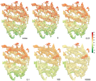
As an illustration, we performed heat kernel smoothing on simulated data. Gaussian noise is added to one of the coordinates (Figure 8). Heat kernel smoothing is performed on the noise added coordinate. Numbers in Figure 8 are kernel bandwidths. At , heat kernel smoothing is equivalent to Fourier series expansion. Thus, we get the almost identical result. As the bandwidth increases, smoothing converges to the mean value. Each disconnected regions should converge to their own different mean values. Thus, when , the regions that are different colors are regions that are disconnected. This phenomena is related to the hot spots conjecture in differential geometry (Banuelos & Burdzy 1999; Chung et al. 2011).The number of disconnected structures can be obtained counting the zero eigenvalues.
The technique can be used to extract the skeleton representation of vessel trees. We perform heat kernel smoothing on node coordinates with . Then rounded off the smoothed coordinates to the nearest integers. The rounded off coordinates were used to reconstruct the binary segmentation. This gives the thick trees in Figure 9 (top left). To obtain thinner trees, the smoothed coordinates were scaled by the factor of 2, 4 and 6 times before rounding off. This had the effect of increasing the image size relative to the kernel bandwidth thus obtaining the skeleton representation of the complex blood vessel (Figure 9 clockwise from top right) (Lindvere et al. 2013; Cheng et al. 2014). By connecting the voxels sequentially, we can obtain the graph representation of the skeleton as well. The method can be easily adopted for obtaining the skeleton representation of complex brain network patterns.
6.5 Diffusion wavelets
Consider a traditional wavelet basis obtained from a mother wavelet with scale and translation parameters and in Euclidean space (Kim et al. 2012):
| (28) |
The wavelet transform of a signal is given by kernel
Scaling a function on an arbitrary manifold including graph is trivial. But the difficulty arises when one tries to translate a mother wavelet. It is not straightforward to generalize the Euclidean formulation (28) to an arbitrary manifold, due to the lack of regular grids (Nain et al. 2007; Bernal-Rusiel et al. 2008). The recent work based on the diffusion wavelet bypasses this problem also by taking bivariate kernel as a mother wavelet (Antoine et al. 2010; Hammond et al. 2011; Mahadevan & Maggioni 2006; Kim et al. 2012). By simply changing the second argument of the kernel, it has the effect of translating the kernel. The diffusion wavelet construction has been fairly involving so far. However, it can be shown to be a special case of the heat kernel regression with proper normalization. Following the notations in Antoine et al. 2010; Hammond et al. 2011; Kim et al. 2012, diffusion wavelet at position and scale is given by
for some scale function . If we let , the diffusion wavelet transform is given by
| (29) | |||||
where is the Fourier coefficient. Note (29) is the kernel regression (Chung et al. 2015). Hence, the diffusion wavelet transform can be simply obtained by doing the kernel regression without an additional wavelet machinery as done in Kim et al. 2012. Further, if we let , we have
which is a heat kernel. The bandwidth of heat kernel controls resolution while the translation is done by shifting one argument in the kernel.
7 Laplace equation
In this section, we will show how to solve for steady state of diffusion. The distribution of fictional charges within the two boundaries sets up a scalar potential field , which satisfies the Poisson equation
where is the total charge within the boundaries. If we set up the two boundaries at different potential, say at and , without enclosing any charge, we have the Laplace equation
The Laplace equation can be viewed as the steady state of diffusion
when . By solving the Laplace equation with the two boundary conditions, we obtain the potential field . Then the electric field perpendicular to the isopotential surfaces is given by . The Laplace equation is mainly solved using the finite difference scheme (Chung 2012). The electric field lines radiate from one conducting surface to the other without crossing each other. By tracing the electric field lines, we obtain one-to-one smooth map between surfaces (Figure 10). The underlying framework is identical to the Laplace equation based surface flattening or cortical thickness estimation (Jones et al. 2000; Chung et al. 2010).

7.1 Glerkin’s method for solving Laplace equation
Without using the finite difference scheme, we can use an analytic approach for solving the Laplace equation using Galerkin’s method (Kirby 2000). Galerkin’s method discretizes partial differential equations and integral equations as a collection of linear equations involving basis functions. The linear equations are then usually solved in the least squares fashion. The iterative residual fitting (IRF) algorithm (Chung et al. 2007; Chung et al. 2008), which iteratively fits functional data using diffusion equations, can be considered as a special case of Glerkin’s method.
We assume the eigenfunctions of satisfying
are available. The solution of the Laplace equation is then approximated as a finite expansion
Consider following boundary conditions
| (30) |
where and are the subregions of . and can be 3D objects, 2D surfaces, graphs or networks. The integral curve between and will establish one to one correspondence.
The boundary conditions satisfy
| (31) |
and
| (32) |
In the interior region , by taking the Laplacian on the expansion , we have
| (33) |
We assume that there are and number of points for equations (31), (32) and (33) respectively. We now combine linear equations (31), (32) and (33) together in a matrix form:
The size of matrix is . is invertible if we sample substantially large number of points . This is likely to be true in medical images so there is no need to use the pseudo-inverse here. Then the matrix equation can be solved by the least squares method:
7.2 Laplace equation with graphs
We can solve for the Laplace equation within a graph . We pick and to be subgraphs of . For instance, we can take and at the two nodes in the graph and solve for the Laplace equation. With the boundary condition and , we are basically solving for steady state heat diffusion between heat source and heat sink .
Instead of solving the Laplace equation within a graph, we can also solve it between graphs by taking and to be two different graphs. For instance, we can take two correlation matrices and , which can be viewed as weighted complete graphs. If we take as the Hodge Laplacian defined on edges (Anand et al. 2021), we can solve the Laplace equation with two correlation matrices as boundary conditions. This provides smooth one-to-one mapping between two correlation matrices. Unlike the usual element wise matching of and , it provides the mapping through heat flow.
Acknowledgements
The part of this study was supported by NIH grants NIH R01 EB022856 and R01 EB028753, NSF grant MDS-2010778. We would like to thank Yuan Wang of University of South Carolina for the providing Gibbs phenomenon plot and Gurong Wu of University of Norh Carolina for providing lung CT scans.
References
- (1)
- Anand et al. (2021) Anand, D., , Dakurah, S., Wang, B. & Chung, M. (2021), ‘Hodge-Laplacian of brain networks and its application to modeling cycles’, arXiv preprint 2110.14599 .
- Andrade et al. (2001) Andrade, A., Kherif, F., Mangin, J., Worsley, K., Paradis, A., Simon, O., Dehaene, S., Le Bihan, D. & Poline, J.-B. (2001), ‘Detection of fMRI activation using cortical surface mapping’, Human Brain Mapping 12, 79–93.
- Antoine et al. (2010) Antoine, J.-P., Roşca, D. & Vandergheynst, P. (2010), ‘Wavelet transform on manifolds: old and new approaches’, Applied and Computational Harmonic Analysis 28, 189–202.
- Banuelos & Burdzy (1999) Banuelos, R. & Burdzy, K. (1999), ‘On the Hot Spots Conjecture of J Rauch’, Journal of Functional Analysis 164, 1–33.
- Belkin et al. (2006) Belkin, M., Niyogi, P. & Sindhwani, V. (2006), ‘Manifold regularization: A geometric framework for learning from labeled and unlabeled examples’, The Journal of Machine Learning Research 7, 2399–2434.
- Bernal-Rusiel et al. (2008) Bernal-Rusiel, J., Atienza, M. & Cantero, J. (2008), ‘Detection of focal changes in human cortical thickness: Spherical wavelets versus gaussian smoothing’, NeuroImage 41, 1278–1292.
- Bronstein & Kokkinos (2010) Bronstein, M. M. & Kokkinos, I. (2010), Scale-invariant heat kernel signatures for non-rigid shape recognition, in ‘IEEE Conference on Computer Vision and Pattern Recognition (CVPR)’, pp. 1704–1711.
- Bulow (2004) Bulow, T. (2004), ‘Spherical diffusion for 3D surface smoothing’, IEEE Transactions on Pattern Analysis and Machine Intelligence 26, 1650–1654.
- Cachia, Mangin, Riviére, Kherif, Boddaert, Andrade, Papadopoulos-Orfanos, Poline, Bloch, Zilbovicius, Sonigo, Brunelle & Régis (2003) Cachia, A., Mangin, J.-F., Riviére, D., Kherif, F., Boddaert, N., Andrade, A., Papadopoulos-Orfanos, D., Poline, J.-B., Bloch, I., Zilbovicius, M., Sonigo, P., Brunelle, F. & Régis, J. (2003), ‘A primal sketch of the cortex mean curvature: A morphogenesis based approach to study the variability of the folding patterns’, IEEE Transactions on Medical Imaging 22, 754–765.
- Cachia, Mangin, Riviére, Papadopoulos-Orfanos, Kherif, Bloch & Régis (2003) Cachia, A., Mangin, J.-F., Riviére, D., Papadopoulos-Orfanos, D., Kherif, F., Bloch, I. & Régis, J. (2003), ‘A generic framework for parcellation of the cortical surface into gyri using geodesic Voronoï diagrams’, Image Analysis 7, 403–416.
- Castillo et al. (2009) Castillo, R., Castillo, E., Guerra, R., Johnson, V., McPhail, T., Garg, A. & Guerrero, T. (2009), ‘A framework for evaluation of deformable image registration spatial accuracy using large landmark point sets’, Physics in medicine and biology 54, 1849–1870.
- Cheng et al. (2014) Cheng, L., De, J., Zhang, X., Lin, F. & Li, H. (2014), Tracing retinal blood vessels by matrix-forest theorem of directed graphs, in ‘International Conference on Medical Image Computing and Computer Assisted Intervention’, Springer, pp. 626–633.
- Chung & Yau (1997) Chung, F. & Yau, S. (1997), ‘Eigenvalue inequalities for graphs and convex subgraphs’, Communications in Analysis and Geometry 5, 575–624.
- Chung (2001) Chung, M. (2001), Statistical Morphometry in Neuroanatomy, Ph.D. Thesis, McGill University. http://www.stat.wisc.edu/~mchung/papers/thesis.pdf.
- Chung (2012) Chung, M. (2012), Computational Neuroanatomy: The Methods, World Scientific, Singapore.
- Chung et al. (2007) Chung, M., Dalton, K., Shen, L., Evans, A. & Davidson, R. (2007), ‘Weighted Fourier representation and its application to quantifying the amount of gray matter’, IEEE Transactions on Medical Imaging 26, 566–581.
- Chung et al. (2008) Chung, M., Hartley, R., Dalton, K. & Davidson, R. (2008), ‘Encoding cortical surface by spherical harmonics’, Statistica Sinica 18, 1269–1291.
- Chung et al. (2015) Chung, M., Qiu, A., Seo, S. & Vorperian, H. (2015), ‘Unified heat kernel regression for diffusion, kernel smoothing and wavelets on manifolds and its application to mandible growth modeling in CT images’, Medical Image Analysis 22, 63–76.
- Chung, Robbins, Dalton, Davidson, Alexander & Evans (2005) Chung, M., Robbins, S., Dalton, K., Davidson, R., Alexander, A. & Evans, A. (2005), ‘Cortical thickness analysis in autism with heat kernel smoothing’, NeuroImage 25, 1256–1265.
- Chung, Robbins & Evans (2005) Chung, M., Robbins, S. & Evans, A. (2005), ‘Unified statistical approach to cortical thickness analysis’, Information Processing in Medical Imaging (IPMI), Lecture Notes in Computer Science 3565, 627–638.
- Chung et al. (2011) Chung, M., Seo, S., Adluru, N. & Vorperian, H. (2011), Hot spots conjecture and its application to modeling tubular structures, in ‘International Workshop on Machine Learning in Medical Imaging’, Vol. 7009, pp. 225–232.
- Chung & Taylor (2004) Chung, M. & Taylor, J. (2004), Diffusion smoothing on brain surface via finite element method, in ‘Proceedings of IEEE International Symposium on Biomedical Imaging (ISBI)’, Vol. 1, pp. 432–435.
- Chung et al. (2018) Chung, M., Wang, Y. & Wu, G. . (2018), ‘Heat kernel smoothing in irregular image domains’, International Conference of the IEEE Engineering in Medicine and Biology Society (EMBC) pp. 5101–5104.
- Chung et al. (2010) Chung, M., Worsley, K., Brendon, M., Dalton, K. & Davidson, R. (2010), ‘General multivariate linear modeling of surface shapes using SurfStat’, NeuroImage 53, 491–505.
- Chung, Worsley, Robbins & Evans (2003) Chung, M., Worsley, K., Robbins, S. & Evans, A. (2003), Tensor-based brain surface modeling and analysis, in ‘IEEE Conference on Computer Vision and Pattern Recognition (CVPR)’, Vol. I, pp. 467–473.
- Chung, Worsley, Robbins, Paus, Taylor, Giedd, Rapoport & Evans (2003) Chung, M., Worsley, K., Robbins, S., Paus, T., Taylor, J., Giedd, J., Rapoport, J. & Evans, A. (2003), ‘Deformation-based surface morphometry applied to gray matter deformation’, NeuroImage 18, 198–213.
- Chung et al. (2001) Chung, M., Worsley, K., Taylor, J., Ramsay, J., Robbins, S. & Evans, A. (2001), ‘Diffusion smoothing on the cortical surface’, NeuroImage 13, S95.
- Courant & Hilbert (1953) Courant, R. & Hilbert, D. (1953), Methods of Mathematical Physics, English edn, Interscience, New York.
- de Goes et al. (2008) de Goes, F., Goldenstein, S. & Velho, L. (2008), ‘A hierarchical segmentation of articulated bodies’, Computer Graphics Forum 27, 1349–1356.
- Fiedler (1973) Fiedler, M. (1973), ‘Algebraic connectivity of graphs’, Czechoslovak Mathematical Journal 23, 298–305.
- Frangi et al. (1998) Frangi, A., Niessen, W., Vincken, K. & Viergever, M. (1998), Multiscale vessel enhancement filtering, in ‘International Conference on Medical Image Computing and Computer-Assisted Intervention’, Vol. 1496, pp. 130–137.
- Gladwell & Zhu (2002) Gladwell, G. & Zhu, H. (2002), ‘Courant’s nodal line theorem and its discrete counterparts’, The Quarterly Journal of Mechanics and Applied Mathematics 55, 1–15.
- Hall (1970) Hall, K. (1970), ‘An r-dimensional quadratic placement algorithm’, Management Science 17, 219–229.
- Ham et al. (2004) Ham, J., Lee, D., Mika, S. & Schölkopf, B. (2004), A kernel view of the dimensionality reduction of manifolds, in ‘Proceedings of the Twenty-first International Conference on Machine Learning’, p. 47.
- Ham et al. (2005) Ham, J., Lee, D. & Saul, L. (2005), Semisupervised alignment of manifolds, in ‘Proceedings of the Annual Conference on Uncertainty in Artificial Intelligence’, Vol. 10, pp. 120–127.
- Hammond et al. (2011) Hammond, D., Vandergheynst, P. & Gribonval, R. (2011), ‘Wavelets on graphs via spectral graph theory’, Applied and Computational Harmonic Analysis 30, 129–150.
- Han et al. (2006) Han, X., Jovicich, J., Salat, D., van der Kouwe, A., Quinn, B., Czanner, S., Busa, E., Pacheco, J., Albert, M., Killiany, R. et al. (2006), ‘Reliability of MRI-derived measurements of human cerebral cortical thickness: The effects of field strength, scanner upgrade and manufacturer’, NeuroImage 32, 180–194.
- Holzrichter & Oliveira (1999) Holzrichter, M. & Oliveira, S. (1999), ‘A graph based method for generating the Fiedler vector of irregular problems’, Parallel and Distributed Processing, Lecture Notes in Computer Science (LNCS) 1586, 978–985.
- Huang et al. (2020) Huang, S.-G., Lyu, I., Qiu, A. & Chung, M. (2020), ‘Fast polynomial approximation of heat kernel convolution on manifolds and its application to brain sulcal and gyral graph pattern analysis’, IEEE Transactions on Medical Imaging 39, 2201–2212.
- Jones et al. (2000) Jones, S., Buchbinder, B. & Aharon, I. (2000), ‘Three-dimensional mapping of cortical thickness using Laplace’s equation’, Human Brain Mapping 11, 12–32.
- Joshi et al. (2009) Joshi, A., Shattuck, D. W., Thompson, P. M. & Leahy, R. M. (2009), ‘A parameterization-based numerical method for isotropic and anisotropic diffusion smoothing on non-flat surfaces’, IEEE Transactions on Image Processing 18, 1358–1365.
- Kim et al. (2012) Kim, W., Pachauri, D., Hatt, C., Chung, M., Johnson, S. & Singh, V. (2012), Wavelet based multi-scale shape features on arbitrary surfaces for cortical thickness discrimination, in ‘Advances in Neural Information Processing Systems’, pp. 1250–1258.
- Kirby (2000) Kirby, M. (2000), Geometric Data Analysis: An empirical approach to dimensionality reduction and the study of patterns, John Wiley Sons, Inc. New York, NY, USA.
- Koren & Harel (2002) Koren, Y. & Harel, D. (2002), ‘A multi-scale algorithm for the linear arrangement problem’, 2573, 296–309.
- Korfiatis et al. (2011) Korfiatis, P., Kalogeropoulou, C., Karahaliou, A., Kazantzi, A. & Costaridou, L. (2011), ‘Vessel tree segmentation in presence of interstitial lung disease in MDCT’, IEEE Transactions on Information Technology in Biomedicine 15, 214–220.
- Lehoucq & Sorensen (1996) Lehoucq, R. & Sorensen, D. (1996), ‘Deflation techniques for an implicitly restarted arnoldi iteration’, SIAM Journal on Matrix Analysis and Applications 17, 789–821.
- Lévy (2006) Lévy, B. (2006), Laplace-Beltrami eigenfunctions towards an algorithm that “understands” geometry, in ‘IEEE International Conference on Shape Modeling and Applications’, p. 13.
- Lindvere et al. (2013) Lindvere, L., Janik, R., Dorr, A., Chartash, D., Sahota, B., Sled, J. & Stefanovic, B. (2013), ‘Cerebral microvascular network geometry changes in response to functional stimulation’, NeuroImage 71, 248–259.
- Mahadevan & Maggioni (2006) Mahadevan, S. & Maggioni, M. (2006), ‘Value function approximation with diffusion wavelets and laplacian eigenfunctions’, Advances in Neural Information Processing Systems 18, 843.
- Malladi & Ravve (2002) Malladi, R. & Ravve, I. (2002), Fast difference schemes for edge enhancing Beltrami flow, in ‘Proceedings of Computer Vision-ECCV, Lecture Notes in Computer Science (LNCS)’, Vol. 2350, pp. 343–357.
- Nain et al. (2007) Nain, D., Styner, M., Niethammer, M., Levitt, J., Shenton, M., Gerig, G., Bobick, A. & Tannenbaum, A. (2007), Statistical shape analysis of brain structures using spherical wavelets, in ‘IEEE Symposium on Biomedical Imaging ISBI’, Vol. 4, pp. 209–212.
- Nilsson et al. (2007) Nilsson, J., Sha, F. & Jordan, M. (2007), Regression on manifolds using kernel dimension reduction, in ‘Proceedings of the 24th international conference on Machine learning’, ACM, pp. 697–704.
- Perona & Malik (1990) Perona, P. & Malik, J. (1990), ‘Scale-space and edge detection using anisotropic diffusion’, IEEE Trans. Pattern Analysis and Machine Intelligence 12, 629–639.
- S. & H. (2008) S., F. & H., M. (2008), ‘Non-parametric regression between manifolds’, Advances in Neural Information Processing Systems 21, 1561–1568.
- Schölkopf & Smola (2002) Schölkopf, B. & Smola, A. J. (2002), Learning with Kernels: Support Vector Machines, Regularization, Optimization, and Beyond, MIT Press.
- Shang et al. (2011) Shang, Y., Deklerck, R., Nyssen, E., Markova, A., de Mey, J., Yang, X. & Sun, K. (2011), ‘Vascular active contour for vessel tree segmentation’, IEEE Transactions on Biomedical Engineering 58, 1023–1032.
- Shawe-Taylor & Cristianini (2004) Shawe-Taylor, J. & Cristianini, N. (2004), Kernel methods for pattern analysis, Cambridge University Press.
- Sochen et al. (1998) Sochen, N., Kimmel, R. & Malladi, R. (1998), ‘A general framework for low level vision’, IEEE Transactions on Image Processing 7, 310–318.
- Sun et al. (2009) Sun, J., Ovsjanikov, M. & Guibas, L. J. (2009), ‘A concise and provably informative multi-scale signature based on heat diffusion.’, Comput. Graph. Forum 28, 1383–1392.
- Tang et al. (1999) Tang, B., Sapiro, G. & Caselles, V. (1999), Direction diffusion, in ‘The Proceedings of the Seventh IEEE International Conference on Computer Vision’, pp. 2:1245–1252.
- Taubin (2000) Taubin, G. (2000), Geometric signal processing on polygonal meshes, in ‘EUROGRAPHICS’, Eurographics Association.
- Tlusty (2007) Tlusty, T. (2007), ‘A relation between the multiplicity of the second eigenvalue of a graph Laplacian, Courant’s nodal line theorem and the substantial dimension of tight polyhedral surfaces’, Electrnoic Journal of Linear Algebra 16, 315–24.
- Wang et al. (2018) Wang, Y., Ombao, H. & Chung, M. (2018), ‘Topological data analysis of single-trial electroencephalographic signals’, Annals of Applied Statistics 12, 1506–1534.
- Wu et al. (2013) Wu, G., Wang, Q., Lian, J. & Shen, D. (2013), ‘Estimating the 4d respiratory lung motion by spatiotemporal registration and super-resolution image reconstruction’, Medical physics 40(3), 031710.
- Yger & Rakotomamonjy (2011) Yger, F. & Rakotomamonjy, A. (2011), ‘Wavelet kernel learning’, Pattern Recognition 44(10-11), 2614–2629.