Persistent Friedel oscillations in Graphene due to a weak magnetic field
Abstract
Two opposite chiralities of Dirac electrons in a 2D graphene sheet modify the Friedel oscillations strongly: electrostatic potential around an impurity in graphene decays much faster than in 2D electron gas. At distances much larger than the de Broglie wavelength, it decays as . Here we show that a weak uniform magnetic field affects the Friedel oscillations in an anomalous way. It creates a field-dependent contribution which is dominant in a parametrically large spatial interval , where is the magnetic length, is Fermi momentum and . Moreover, in this interval, the field-dependent oscillations do not decay with distance. The effect originates from a spin-dependent magnetic phase accumulated by the electron propagator. The obtained phase may give rise to novel interaction effects in transport and thermodynamic characteristics of graphene and graphene-based heterostructures.
I introduction
Graphene, a single-atom-thick honeycomb sheet of carbon atomsNovoselov et al. 2004; Novoselov et al. 2005, possesses unusual material characteristics as compared to other 2D electron systems. Having high electron mobilities, the particles in Graphene are orders of magnitude faster than in silicon; they conduct heat much more efficiently than in diamond and conduct current order of magnitude better than in copper. Among other unique properties, Graphene is transparent and impermeable to most gases and liquids, including heliumSun et al. 2020. It is harder than diamond and more elastic than fiber carbon at the same time.
Unique electronic properties of GrapheneZhang et al. 2005; Gusynin and Sharapov 2005; Wunsch et al. 2006; Altland 2006; Cheianov and Fal’ko 2006; Aleiner and Efetov 2006; Tworzydło et al. 2006; Rycerz et al. 2007; Beenakker 2008; Tan et al. 2007; Mariani et al. 2007; Tse et al. 2008; Bena 2008; Bena 2009; Castro Neto et al. 2009; Bolotin et al. 2009; Bena 2010; Vozmediano et al. 2010; Bácsi and Virosztek 2010; Gómez-Santos and Stauber 2011; Goerbig 2011; Vaishnav et al. 2011; Das Sarma et al. 2011; Kotov et al. 2012; Semenoff 2012; Nandkishore et al. 2012; Dutreix et al. 2013; Lawlor et al. 2013; Amorim et al. 2016; Rusin and Zawadzki 2018; Dutreix et al. 2019; Agarwal and Mishchenko 2020; Sedrakyan et al.; Maiti and Sedrakyan 2019; Sun et al. 2020 stem from the fact that it is single-atom-thick. It supports carriers with Dirac-like dispersion. When doping is low, the Fermi level is located in the close vicinity of and points in the Brillouin zone. The reason for this is that Graphene quasiparticles possess chiral properties related to the two-sublattice structure of the honeycomb lattice. The latter also implies that the lattice unit cell contains two sites (atoms), leading to a “pseudospin” degree of freedom.
One of the most prominent effects in regular 2D electron systems is the interaction-induced zero-bias anomaly in the tunnel density of states (DOS). For small impurity concentration, this anomaly can be traced to the factRudin et al. 1997 that impurities are dressed with Friedel oscillations of the electron densityFriedel 1952 which falls off as with distance, , from the impurity. Modification of the wave functions due to scattering of electrons from the dressed impurities gives rise to the singular correction to the self-energy. Upon the advent of Graphene, the calculations similar to that in 2D gas,Cheianov and Fal’ko 2006; Wunsch et al. 2006; Mariani et al. 2007 indicated that the zero-bias anomaly in Graphene is absent. The underlying reason for this absence is that, with matrix underlying Hamiltonian of spin-orbit type, the backscattering of electrons is forbiddenChen and Raikh 1999. As a result, the Friedel oscillations in Graphene falls off faster than in 2D gas, as .
Since Refs. Cheianov and Fal’ko 2006; Mariani et al. 2007; Wunsch et al. 2006 the Friedel oscillations in Graphene were studied in tiniest details, both analytically within continuum approximation and numerically, within tight-binding approximation. The results are summarized in the reviewBena 2016.
Application of a magnetic field turns the spectrum of Graphene into a ladder of non-equidistant Landau levels. The corresponding perturbation of the electron density around an impurity can be cast into a sum over these levelsBena 2016; Rusin and Zawadzki 2018. Still, at elevated temperatures, the discreteness of the Landau levels does not manifest itself, and the behavior of the Friedel oscillations with distance becomes quite a nontrivial issue. A natural expectation is that a weak, non-quantizing magnetic field, modifies the Friedel oscillations in Graphene in the same way as in the 2D electron gasSedrakyan et al. 2007. By causing the curving of the semiclassical trajectories, the field gives rise to the position-dependent magnetic phase, and, thus, breaks the periodicity of the oscillations. Still, the decay law of the oscillations remains the same as in a zero field. In fact, such an intuitive reasoning, in application to Graphene, is wrong. It is not only the phase but also the magnitude of the Friedel oscillations that exhibits a crucial dependence on the magnetic field.
In the present paper we consider this question systematically and find the field-dependent form of the Friedel oscillations. We shed light on the nature of the magnetic field modification. Our key finding is that the potential oscillates anomalously. Namely, it does not fall off with distance, , in a parametrically large interval. This omnipresent effect plays a central role in a variety of quantum many-body contexts in Graphene. The polarization operator (PO) is an essential quantity for the evaluation of interaction effects using the Feynman diagrams. The non-decaying part in the PO dramatically changes the power counting in the integrand expressing Feynman diagrams. From the new power counting, the magnetic effect may give rise to a new zero-bias anomaly in DOS of Graphene, modify to the quasi-particle lifetime and thermodynamics of Dirac electrons in the Fermi liquid regime. It may also induce new temperature dependence for the dc/ac conductivitiesWang et al.. The obtained non-decaying Friedel oscillations open an avenue for controlled studies of magnetotransport. They also manifest themselves in field-related thermodynamic properties of Graphene and materials with a pseudo magnetic field such as randomly strained Graphene, stacked and twisted Dirac materials, and the properties of the wormholes in themGonzález and Herrero 2010; Capozziello et al. 2020; Garcia et al. 2020.
The Hamiltonian that incorporates the field in Landau gauge reads ,
| (1) |
where is the short-ranged impurity potential, is the Fermi velocity and . One can define , together with , to form a su(2)-algebra. The Pauli matrices act in the space of and sublattices of the honeycomb lattice, is the Pauli matrix distinguishing between two Dirac points ( and ) of the Graphene dispersion relation and is the identity matrix. We consider the simplest case of the diagonal disorder , where is a scalar. The uniform field breaks the chiral symmetry near each Dirac point individually since, , does not commute with the Hamiltonian. It is this non-commutativity, specific for graphene and other Dirac materialsWehling et al. 2014, that causes the observable modification of Friedel oscillations in a weak magnetic field, . Quantitatively, the criterion of weak field is that the the magnetic length, , is much larger than the de Broglie wavelength, . Below we show that weak field modifies the screened Coulomb potentialYue et al. 1994; Zala et al. 2001; Adamov et al. 2006 to
| (2) |
Here is the component of the interaction, while the impurity potential is treated in the Born approximation with . There are two competing terms. One can see that when the magnetic phase with , the potential is decaying as a polynomial function, . When , the potential is oscillating anomalously, with a constant amplitude. This persistent effect comes from the diagonal part of impurity potential, while other non-magnetic impurity potentials do not contribute to in the leading order in impurity scattering. (for details, see Appendix A and B.)
The paper is organized as follows. In Sec.(II), we present a qualitative derivation of persistent Friedel oscillations, which follows from the semi-classical magnetic phase accumulated by the electron propagator. In Sec.(III), we present a thorough calculation of the polarization operator in the presence of a weak magnetic field and derive Friedel oscillations of electron density. The implications to interaction effects are discussed in Sec.(IV). Concluding remarks are given in Sec.(V).
II Qualitative discussion
In this section, we make a qualitative argument for new effects of Friedel oscillations in Eq. (1). Both modifications of Friedel oscillations, namely the phase in oscillations and the persistent part, can be understood semiclassically. The electron propagator, , where represent sublattices, accumulates a phase, , when electrons propagate along the semi-classical arc. Here is the length of arc shown in the inset of Fig. (1) and is an effective momentum. The diagonal component of Dirac propagator, , can be understood as a propagator of the 2D electron gas with an effective Fermi energy and an effective cyclotron frequency . This yields an effective momentum for diagonal propagators. While if , . For details of deriving effective momentums, see Appendix (C).
The phase in the oscillations is due to the curving of the path. Semiclassically, the propagator acquires a magnetic phase because of the curving of trajectory. Since , and , the magnetic phase becomes equal to . The PO involves a product of two propagators, and thus the magnetic phase in PO is doubled. This is exactly the magnetic phase of Friedel oscillations.
The persistent part of Friedel oscillations originates from the deviation of from . The effective momentum implies spin-dependent magnetic phases, of diagonal propagators . Although the phase is spin-dependent, it does not depend on the valleys. The phase could then be expressed compactly, . The PO involves a trace of two propagators. Using the fact that Pauli matrices are traceless and , the leading magnetic contribution to PO is from a square of , namely . This is the new amplitude of the second term in Eq. (I).
Importantly, the anomalous effect in Eq. (I) persists even at high temperatures, , which is much higher than the cyclotron energy. The temperature scale, can be derived qualitatively. Quasi-classically, the electron propagator accumulates a dynamical phase along the arc (see the inset in Fig. 1). The condition can be cast in the form , since . Then, the spatial scale translates into the energy scale . This, in turn, sets the temperature scale, .
III The Polarization operator
In this section, we show the emergence of persistent Friedel oscillations by calculating the PO rigorously in the momentum space. We start from the summation over Landau levels for PO and then develop a low energy effective theory around the Fermi level. We show how the spin-dependent magnetic phase of the gauge-invariant electron propagator manifests itself in the matrix elements of PO. Using the obtained form of the PO, we derive the Friedel oscillations and observe their persistent behavior. Finally, we discuss the smearing of anomalies in the PO under a weak magnetic field.
III.1 Summation over Landau levels
. We start from a general expression for the PO in the momentum space
| (3) |
where is the Fermi-Dirac distribution, while the frequencies, , are given by . The quantities are the matrix elements of between the states and . Since the wave functions are the vectors consisting of the oscillator states and , the square of the matrix element can be expressed via the generalized Laguerre polynomials, , as follows
where . The summation in Eq. (3) is performed over two valleys and two spins. However, the main contribution comes from the states near the Fermi level, , which we assume to be positive. This allows to set in Eq. (III.1). The condition that the magnetic field is weak can be cast in the form, , where is the number of Landau levels with energies between and .
To perform the summation over and it is convenient to use the following integral representation of the Laguerre polynomials
| (5) |
In the vicinity of the Kohn anomaly, , we have . Under this condition, the major contribution to the integral Eq. (5) comes from the vicinity of . Substituting into the integrand and expanding with respect to yields the following integral representation for the square of the matrix element (details see Appendix D)
| (6) | |||||
Here the spin-dependent magnetic phase, the signal of chiral symmetry breaking, manifests itself in the matrix element as a small, but non-negligible, phases , with . The negative sign in the second line is the result of the Berry phase , which is specific for Dirac electrons. The two features are responsible for the main result of the paper.
Since the main contribution to the sum in Eq. (3) comes from and close to , it is convenient to introduce the new variables , . Then the summation in Eq. (3) can be performed with the help of the following identity
| (7) |
where is the effective cyclotron frequency and , are real numbers. When applying the above identity to the summation in Eq. (3), we set with and . As we will see in the next section, the integration over defines a characteristic scale, . This scale for implies that the temperature damping term is essentially temperature independent at , namely . At , the damping factor is important, as it becomes exponential: . In the following, we work in the low temperature limit, . This effect of persistent oscillation will survive up to , while at higher temperatures the Friedel oscillations will be washed out.
III.2 The form of the PO
Equipped with Eq. (6) and (III.1), one can write the static PO, , as a single integral with respect to variable . Details see Appendix (E). To clarify two different effects in , we present as sum of two terms . Here and are expressed by
| (8) | |||||
and
| (9) | |||||
Here is the momentum measured from . Finite low- cutoff, , of the order of the lattice spacing, does not affect the form of the Friedel oscillations. We will see that and are responsible for the two distinct contributions to the Friedel oscillations in Eq. (I).
Here we derive the PO in the real space. We start with the contribution Eq. (8). Transformation to the real space is accomplished by the following radial integral
| (10) |
where is the zeroth-order Bessel function. Here we have used the fact that . In the domain, , we can replace the Bessel function by the large- asymptote . The integration over sets . Then the summation over in Eq. (8) yields
| (11) | |||||
The effect of the weak magnetic field is not negligible if the magnetic phase . From here, the characteristic scale for is . Since we consider the distances , i.e. much smaller than the Lamour radius, the magnitude of oscillations given by -function in the equation above can be further simplified to . The result for describes the contribution to the oscillations of the electron density which do not decay with distance in the domain . It reproduces the second term in Eq. (I).
Evaluation of the contribution to the PO defined by Eq. (9) involves the same steps as evaluation of . The result reads
| (12) |
It reproduces the first term in Eq. (I). The decay is specific for Graphene, while the phase is the same as in 2D electron gas.
The the real space static PO, , determines the Hartree potential , via modulation of the electron density around the impurity. Within the Born approximation, . Since the density modulation originates from the backscattering of fermions, determines the Hartree potential as (The derivation see Appendix F). As such, the Hartree potential is equivalent to .
III.3 Smeared anomalies
The spin-dependent magnetic phase, , leads to a new term, , in the PO, while the curving of path smears the existing anomaly in . We start from the momentum-space representation of the PO given in terms of the product of the Airy functionsBateman et al. 1953. Then we differentiate Eq. (9) with respect to twice and obtain
| (13) |
where . This represents the smearing of the Kohn anomaly of the PO by the weak field. Inset of Fig. (2) illustrates how the anomaly get smeared.
Importantly, can also be obtained as (details see Appendix G)
| (14) |
This term only emerges in the presence of the magnetic field. In the limit , , it converges to zero as . This asymptote, plotted in Fig. (2), has same origin with persistent oscillations. To better understand the effect, one can Fourier transform using the asymptote. From power counting, it is straightforward to see the emergence of the non-decaying oscillating function, .
IV Implications to interaction effects
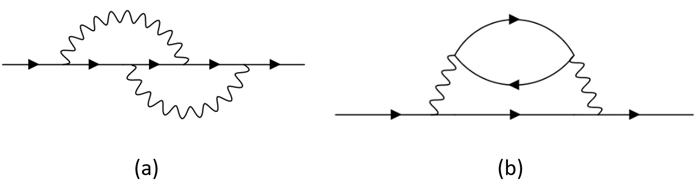
Graphene is a 2D Fermi-liquid when . This implies that the scattering rate of the quasi-particle around Fermi surface obeys . In perturbation theory in interaction parameter, two leading Feynman diagrams contributing to the electron lifetime are shown in Fig. (3). We evaluate these diagrams in the presence of the weak magnetic field using the obtained form of the electron propagator. The computation leads to an unexpected resultWang et al.: the quasiparticle lifetime acquires a singular in magnetic correction Here is the scattering rate of quasi-particle with frequency in the presence of the magnetic field, , . The expression is valid when . The magnetic correction above is more singular in frequency than the non-magnetic part. This singularity originates from the spin-dependent magnetic phase, , in electron propagators. Interestingly, the field-dependent interaction corrections to various observables in Graphene, including zero-bias anomaly in the density of states and ac/dc conductivities, also exhibit more singular behavior in either or temperature, Wang et al..
V Concluding remarks
In this paper we demonstrated that weak magnetic field manifests itself in the Friedel oscillations in two ways: it modifies (i) the phase of the oscillations and (ii) makes the magnitude of oscillations non-decaying in a parametrically large interval. The origin of the modification of the phase in oscillations, , can be traced to the curving of the classical trajectory of an electron in a weak magnetic field (see inset in Fig. 1). The trajectory is curved even at much smaller than the Larmour radius, leading to the magnetic phaseSedrakyan et al. 2007 . This effect just by itself leads to remarkable high-temperature interaction effects in 2DEGSedrakyan and Raikh 2008a; Sedrakyan and Raikh 2008b; Sedrakyan and Raikh 2008c.
Graphene also supports modification of the magnitude of the Friedel oscillations by a weak field. The origin of this effect is an emerging spin-dependent phase in electron propagators, . This effect manifests in persistent Friedel oscillations and leads to non-trivial magnetic corrections to many-body characteristics in Graphene. The transport and thermodynamic properties of monolayer Dirac materials, randomly strained Graphene and stacked and twisted Dirac materials will also be anomalously sensitive to this magnetic phase even at temperatures, , which is much higher than the cyclotron energySedrakyan et al. 2007.
Technically, to develop the theory of interaction effects in Dirac materials in the presence of the weak field, one can use the obtained form of the PO and/or Friedel oscillations in the Feynman diagrams (in the momentum or real space representations). However, a word of caution is in order here. Since the field dependence also enters the fermion Green’s functions, in the Feynman diagrams, one should also consider modified propagators on the same footing along with Friedel oscillations. The explicit form of the Feynman propagators in the weak B-field is derived in Appendix A.
Experimentally, Friedel oscillations can be observed with the scanning tunneling microscope (STM), which images 2D surfaces at the atomic levelSprunger et al. 1997; Dutreix et al. 2019; Stano et al. 2013. In STM, data are determined by backscattering processes along the energy contours. Experimental tests of these oscillations would include examining the temperature dependence of the Friedel oscillations through an extended range of temperatures , determining the persistent range of oscillations, , and investigating the effect of their -dependence.
VI Acknowledgements
. The research was supported by startup funds from the University of Massachusetts, Amherst (K.W. and T.A.S.), and by the Department of Energy, Office of Basic Energy Sciences, Grant No. DE-FG02-06ER46313 (M.E.R.).
Appendix A Real-space calculation of the Friedel oscillations
Consider the modification of the Friedel oscillations in graphene by a weak uniform magnetic field. The Hamiltonian that incorporates the field in Landau gauge reads
| (15) |
with . Here is the short-ranged impurity potential, is the Fermi velocity and . One can define , together with to form a su(2)-algebra. Clearly, the uniform field breaks the chiral symmetry since, in a finite fields, does not commute with . In the following, we report the result for the Green function in the asymptotic region , . Here is given by
| (16) |
where we only preserve the leading orders with the non-quantized condition . Here is the magnetic length, is the Fermi momentum and is the frequency measured from the Fermi energy. We also define functions by
| (17) | |||
where , describe breaking of the translational invariance and is a scale introduced by Sedrakyan, Mishchenko, and Raikh in Ref. Sedrakyan et al. 2007 to characterize the magnetic phase in the Green function of the 2D electron gas.
Having the form of Green’s function in the presence of a weak field, one can calculate the polarization operator.
| (18) | |||||
Here we still consider an impurity with . After putting expression expressions into the equation above, one can obtain the component of the polarization operator
| (19) | |||||
This result fits well with the Eq. (21) and Eq. (22) in the main text, the result obtained in the momentum space. The decay of the first oscillatory term here is consistent with the result of free Dirac electronsWunsch et al. 2006; Cheianov and Fal’ko 2006; Mariani et al. 2007, however there is an additional magnetic phase that breaks periodicity of oscillations. The ratio between magnitudes of the first and the second oscillatory functions is proportional to . When (i) , the polarization operator in real space decays as ; (ii) , the chiral symmetry breaking effect dominates. This symmetry-breaking term is proportional to , i.e., it oscillates with constant amplitude.
Finally, one can evaluate the effective electrostatic potential around the impurity (where we restore spin 1/2 back), which yields
| (20) | |||||
Appendix B Effect of disorder
In the main text, we considered the disorder potential to be , with . Around Eq. (2), we discuss the effects of other disorder potentials on the Hartree potential. This section provides further detailed calculations. Consider a non-magnetic impurity, which should be Hermitian and time-reversal symmetric . Then the could be expressed by ten parametersMcCann et al. 2006; Aleiner and Efetov 2006
| (21) |
where the matrices are given by
| (22) | |||
| (23) |
Here the Pauli matrices are acting on space of the valley indices while the Pauli matrices act in the space of A/B sublattices. Components of impurity potentials are explained as follows:
- •
is the diagonal disorder, the electric-static potential averaged over A/B sublattices.
- •
and introduce the hoppings between A and B.
- •
, introduce the intervalley scatterings, .
- •
defines the difference between on-site chemical potentials on A and B sublattices. It represents the sublattice symmetry breaking mass term.
The polarization operator is given by
Then we define a intermediate matrix, which does not depend on the nature of impurity potentials
After the integration, we find that reads as
| (24) |
where is the second pauli matrix and is defined by
| (25) | |||||
Here . Then the polarization operator is given by
| (26) |
Since is quasi-diagonal, the inter-valley scattering components of the impurity vanish after the trace. So we only need to take , , and into consideration, involving the matrices
Among these impurity potentials, we find that only -component gives non-zero contribution to PO in the leading order
| (27) | |||||
As we can see, only the diagonal disorder gives the persistent Friedel oscillations. Other impurity potentials do not contribute to the polarization operator in the leading order in impurity scattering. In this way, we see that Eq. (2) of main text will remain unchanged in the presence of generic non-magnetic impurity potentials.
Appendix C Derivation of effective momentums
In this section, we give a derivation of effective momentums , mentioned by the qualitative argument from maintext, in the operator formalism (summations over Landau levels). Since and , propagators at valley and , can be connnected by , we will only focus on the calculation of one valley, -valley.
Under a magnetic field, the free Dirac electrons are transformed into ladders of Landau levels. The positive part of landau levels are given by . Here is the Fermi velocity and is the magnetic length. The corresponding wavefunction at -valley is given by , where is the wavefunction of Landau level of 2D electrons. Considering the positive Fermi energy , we only need to consider the Landau levels around . Then from definition of propagators, we get the following expression
| (28) |
Here refer to sublattice and is the step function. The off-diagonal propagtors could be expressed in terms of diagonal ones via the following expression
| (29) |
with . The derivation (see Ref. Rusin and Zawadzki 2018 ) mainly involves the properties of Lagaurre polynomials. Thus we could only focus on the Landau summations for diagonal propagators. One puts the expression of and finds
| (30) |
One can transfer the index into by variable change . This method yields
| (31) |
We expand around the Fermi energy and find
Here it introduce an effective Fermi energy and effective cyclotron frequency . Subsequently, the effective Fermi energy introduces an effective momentum by . One immediately see .
One could use Eq. (29) to find that effective momentum in the off-diagonal Green functions is exactly the Fermi momentum. It indicates that , if . Combining two facts, one could conclude that
| (32) |
Appendix D Details of the calculation of the matrix elements
We start from the integral representation of the Laguerre polynomials
| (33) |
In the vicinity of the Kohn anomaly, , we have . Under this condition, the major contribution to the integral Eq. (5) comes from the vicinity of . Substituting into the integrand and expanding with respect to , we get
| (34) |
where the phase is given by . The last term in the brackets originates from the denominator in Eq. (5) expanded and exponentiated. This term is important since and, thus, .
From Eq. (34), and the form of , we conclude that the integrand in the product contains the phase
| (35) | |||||
while the integrand in the product contains the phase
| (36) | |||||
With the help of Eqs. (35), (36) one gets the integral representation for the square of the matrix element, which is the Eq. (6) in the main text.
Appendix E Details of obtaining the integral representation of the polarization operator
Since the main contribution to the sum in Eq. (3) comes from and close to , it is convenient to introduce the new variables , , so that the relevant , are much smaller than . Note also, that the first terms in Eqs. (35), (36) measure the proximity of the momentum, , to the Kohn anomaly . Indeed, with , we have , where . On other hand, the cubic terms in Eqs. (35), (36) are the smooth functions of , so it is sufficient to replace by in these terms. Using these notations in Eqs. (6), we rewrite the static polarization operator as a sum over and
| (37) | |||
Subsequent steps rely on the relative smallness of , . Using this smallness, we expand as , and replace the difference by . Finally, we extend the summation over and to .
The above simplifications allow to perform the summation over and explicitly. This is achieved with the help of the identity in Eq.(III.1). Upon applying this identity, the polarization operator Eq. (37) acquires the form
| (38) | |||||
Define , . Then the double integral assumes the form
We see that the exponents in both terms are the quadratic forms of . Thus, with respect to , the integrals of both terms are gaussian. The result of the integration reads
Then one could express it as the sum of two terms and to reproduce Eq. (8) and Eq. (9) in the maintext.
Appendix F Relation bewteen the Hartree potential and the static polarization opeartor
The modulation of the electron density, , around the impurity determines the Hartree potential by
| (39) |
Here is the screened Coulomb potential. Since the modulation originates from the backscattering of fermions, oscillates with the momentum . This implies that the Fourier component is nonzero only when . Upon the Fourier expansion of , one obtains
| (40) |
Here we use the expression of that . Since the Coulomb potential is rotational-invariant, . Thus the expression above is further simplified to be
| (41) |
One use the Fourier expansion of and immediately see
| (42) |
In the Born approximation, the modulation of density is estimated by . Here and is the static polarization operator in real space. Finally, one obtains the relation between the static polarization operator and the Hartree potential
| (43) |
Appendix G Details of the calculation of
The first step is to redefine the variable inside the integral of Eq. (15) of the main text
Then Eq. (15) of the main text is now written as the integral over
| (44) | |||||
with the new cut-off . The next step is to take the first derivatve of versus
| (45) | |||||
Here we use the integral expression of product of Airy functions
Then we write as summation of three Airy functions
| (46) |
Since (weak magnetic field), one can take Taylor Expansion of the product of Airy functions
around . Define . Up to the second order perturbation, Eq. (G) is rewritten as
| (47) |
Here, the leading term cancels since
while the first order perturbation also vanishes due to the fact
So the left term is the second order perturbation in the Taylor Expansion
| (48) |
Upon using , we reach
| (49) |
References
- Novoselov et al. (2004) K. S. Novoselov, A. K. Geim, S. V. Morozov, D. Jiang, Y. Zhang, S. V. Dubonos, I. V. Grigorieva, and A. A. Firsov, “Electric field effect in atomically thin carbon films,” Science 306, 666 (2004).
- Novoselov et al. (2005) K. S. Novoselov, A. K. Geim, S. V. Morozov, D. Jiang, M. I. Katsnelson, I. V. Grigorieva, S. V. Dubonos, and A. A. Firsov, “Two-dimensional gas of massless Dirac fermions in graphene,” Nature 438, 197 (2005).
- Sun et al. (2020) P. Z. Sun, Q. Yang, W. J. Kuang, Y. V. Stebunov, W. Q. Xiong, J. Yu, R. R. Nair, M. I. Katsnelson, S. J. Yuan, I. V. Grigorieva, M. Lozada-Hidalgo, F. C. Wang, and A. K. Geim, “Limits on gas impermeability of graphene,” Nature 579, 229 (2020).
- Zhang et al. (2005) Yuanbo Zhang, Yan-Wen Tan, Horst L. Stormer, and Philip Kim, “Experimental observation of the quantum Hall effect and Berry’s phase in graphene,” Nature 438, 201 (2005).
- Gusynin and Sharapov (2005) V. P. Gusynin and S. G. Sharapov, “Unconventional Integer Quantum Hall effect in graphene,” Phys. Rev. Lett. 95, 146801 (2005).
- Wunsch et al. (2006) B. Wunsch, T. Stauber, F. Sols, and F. Guinea, “Dynamical polarization of graphene at finite doping,” New J. of Phys. 8, 318 (2006).
- Altland (2006) A. Altland, “Low-energy theory of disordered graphene,” Phys. Rev. Lett. 97, 236802 (2006).
- Cheianov and Fal’ko (2006) V. V. Cheianov and V. I. Fal’ko, “Friedel Oscillations, impurity scattering, and temperature dependence of resistivity in graphene,” Phys. Rev. Lett. 97, 226801 (2006).
- Aleiner and Efetov (2006) I. L. Aleiner and K. B. Efetov, “Effect of disorder on transport in graphene,” Phys. Rev. Lett. 97, 236801 (2006).
- Tworzydło et al. (2006) J. Tworzydło, B. Trauzettel, M. Titov, A. Rycerz, and C. W. J. Beenakker, “Sub-poissonian shot noise in graphene,” Phys. Rev. Lett. 96, 246802 (2006).
- Rycerz et al. (2007) A. Rycerz, J. Tworzydło, and C. W. J. Beenakker, “Valley filter and valley valve in graphene,” Nature Physics 3, 172 (2007).
- Beenakker (2008) C. W. J. Beenakker, “Colloquium: Andreev reflection and klein tunneling in graphene,” Rev. Mod. Phys. 80, 1337 (2008).
- Tan et al. (2007) Y.-W. Tan, Y. Zhang, K. Bolotin, Y. Zhao, S. Adam, E. H. Hwang, S. Das Sarma, H. L. Stormer, and P. Kim, “Measurement of scattering rate and minimum conductivity in graphene,” Phys. Rev. Lett. 99, 246803 (2007).
- Mariani et al. (2007) E. Mariani, L. I. Glazman, A. Kamenev, and F. von Oppen, “Zero-bias anomaly in the tunneling density of states of graphene,” Phys. Rev. B 76, 165402 (2007).
- Tse et al. (2008) Wang-Kong Tse, Ben Yu-Kuang Hu, and S. Das Sarma, “Chirality-induced dynamic Kohn Anomalies in graphene,” Phys. Rev. Lett. 101, 066401 (2008).
- Bena (2008) C. Bena, “Effect of a single localized impurity on the local density of states in monolayer and bilayer graphene,” Phys. Rev. Lett. 100, 076601 (2008).
- Bena (2009) C. Bena, “Green’s functions and impurity scattering in graphene,” Phys. Rev. B 79, 125427 (2009).
- Castro Neto et al. (2009) A. H. Castro Neto, F. Guinea, N. M. R. Peres, K. S. Novoselov, and A. K. Geim, “The electronic properties of graphene,” Rev. Mod. Phys. 81, 109 (2009).
- Bolotin et al. (2009) Kirill I. Bolotin, Fereshte Ghahari, Michael D. Shulman, Horst L. Stormer, and Philip Kim, “Observation of the fractional quantum Hall effect in graphene,” Nature 462, 196 (2009).
- Bena (2010) C. Bena, “Local density of states in the presence of impurity scattering in graphene at high magnetic field,” Phys. Rev. B 81, 045409 (2010).
- Vozmediano et al. (2010) M. A. H. Vozmediano, M. I. Katsnelson, and F. Guinea, “Gauge fields in graphene,” Phys. Rep. 496, 109 (2010).
- Bácsi and Virosztek (2010) Á. Bácsi and A. Virosztek, “Local density of states and Friedel oscillations in graphene,” Phys. Rev. B 82, 193405 (2010).
- Gómez-Santos and Stauber (2011) G. Gómez-Santos and T. Stauber, “Measurable lattice effects on the charge and magnetic response in graphene,” Phys. Rev. Lett. 106, 045504 (2011).
- Goerbig (2011) M. O. Goerbig, “Electronic properties of graphene in a strong magnetic field,” Rev. Mod. Phys. 83, 1193 (2011).
- Vaishnav et al. (2011) J. Y. Vaishnav, J. Q. Anderson, and J. D. Walls, “Intravalley multiple scattering of quasiparticles in graphene,” Phys. Rev. B 83, 165437 (2011).
- Das Sarma et al. (2011) S. Das Sarma, S. Adam, E. H. Hwang, and E. Rossi, “Electronic transport in two-dimensional graphene,” Rev. Mod. Phys. 83, 407 (2011).
- Kotov et al. (2012) V. N. Kotov, B. Uchoa, V. M. Pereira, F. Guinea, and A. H. Castro Neto, “Electron-electron interactions in graphene: Current status and perspectives,” Rev. Mod. Phys. 84, 1067 (2012).
- Semenoff (2012) G. W. Semenoff, “Chiral symmetry breaking in graphene,” Phys. Scr. T146, 014016 (2012).
- Nandkishore et al. (2012) R. Nandkishore, L. S. Levitov, and A. V. Chubukov, “Chiral superconductivity from repulsive interactions in doped graphene,” Nature Physics 8, 158 (2012).
- Dutreix et al. (2013) C. Dutreix, L. Bilteanu, A. Jagannathan, and C. Bena, “Friedel oscillations at the Dirac cone merging point in anisotropic graphene and graphenelike materials,” Phys. Rev. B 87, 245413 (2013).
- Lawlor et al. (2013) J. A. Lawlor, S. R. Power, and M. S. Ferreira, “Friedel oscillations in graphene: Sublattice asymmetry in doping,” Phys. Rev. B 88, 205416 (2013).
- Amorim et al. (2016) B. Amorim, A. Cortijo, F. de Juan, A. G. Grushin, F. Guinea, A. Gutiérrez-Rubio, H. Ochoa, V. Parente, R. Roldán, P. San-Jose, J. Schiefele, M. Sturla, and M. A. H. Vozmediano, “Novel effects of strains in graphene and other two dimensional materials,” Phys. Rep. 617, 1 (2016).
- Rusin and Zawadzki (2018) T. M. Rusin and W. Zawadzki, “Theory of Friedel oscillations in monolayer graphene and group-vi dichalcogenides in a magnetic field,” Phys. Rev. B 97, 205410 (2018).
- Dutreix et al. (2019) C. Dutreix, H. González-Herrero, I. Brihuega, M. I. Katsnelson, C. Chapelier, and V. T. Renard, “Measuring the Berry phase of graphene from wavefront dislocations in Friedel oscillations,” Nature 574, 219 (2019).
- Agarwal and Mishchenko (2020) M. Agarwal and E. G. Mishchenko, “Dynamic response functions of two-dimensional Dirac fermions with screened coulomb and short-range interactions,” Phys. Rev. B 102, 125421 (2020).
- (36) A. Sedrakyan, A. Sinner, and K. Ziegler, “Deformation of graphene sheet: Interaction of fermions with phonons,” arXiv:2007.08372.
- Maiti and Sedrakyan (2019) S. Maiti and T. A. Sedrakyan, “Composite fermion state of graphene as a Haldane-Chern insulator,” Phys. Rev. B 100, 125428 (2019).
- Rudin et al. (1997) A. M. Rudin, I. L. Aleiner, and L. I. Glazman, “Tunneling zero-bias anomaly in the quasiballistic regime,” Phys. Rev. B 55, 9322 (1997).
- Friedel (1952) J. Friedel, Phil. Mag. 43, 153 (1952).
- Chen and Raikh (1999) Guang-Hong Chen and M. E. Raikh, “Small- anomaly in the dielectric function and high-temperature oscillations of the screening potential in a two-dimensional electron gas with spin-orbit coupling,” Phys. Rev. B 59, 5090 (1999).
- Bena (2016) C. Bena, “Friedel oscillations: Decoding the hidden physics,” Comptes Rendus Physique 17, 302 (2016).
- Sedrakyan et al. (2007) T. A. Sedrakyan, E. G. Mishchenko, and M. E. Raikh, “Smearing of the two-dimensional Kohn Anomaly in a nonquantizing magnetic field: Implications for interaction effects,” Phys. Rev. Lett. 99, 036401 (2007).
- (43) Ke Wang, M. E. Raikh, and T. A. Sedrakyan, Unpublished .
- González and Herrero (2010) J. González and J. Herrero, “Graphene wormholes: A condensed matter illustration of Dirac fermions in curved space,” Nucl. Phys. B 825, 426 (2010).
- Capozziello et al. (2020) S. Capozziello, R. Pincak, and E. Bartoš, “Chern-Simons current of left and right chiral superspace in graphene wormhole,” Symmetry 12, 774 (2020).
- Garcia et al. (2020) G. Q. Garcia, P. J. Porfírio, D. C. Moreira, and C. Furtado, “Graphene wormhole trapped by external magnetic field,” Nucl. Phys. B 950, 114853 (2020).
- Wehling et al. (2014) T.O. Wehling, A.M. Black-Schaffer, and A.V. Balatsky, “Dirac materials,” Adv. Phys. 63, 1 (2014).
- Yue et al. (1994) Dongxiao Yue, L. I. Glazman, and K. A. Matveev, “Conduction of a weakly interacting one-dimensional electron gas through a single barrier,” Phys. Rev. B 49, 1966 (1994).
- Zala et al. (2001) Gábor Zala, B. N. Narozhny, and I. L. Aleiner, “Interaction corrections at intermediate temperatures: Longitudinal conductivity and kinetic equation,” Phys. Rev. B 64, 214204 (2001).
- Adamov et al. (2006) Y. Adamov, I. V. Gornyi, and A. D. Mirlin, “Interaction effects on magneto-oscillations in a two-dimensional electron gas,” Phys. Rev. B 73, 045426 (2006).
- Bateman et al. (1953) H. Bateman, A. Erdélyi, W. Magnus, F. Oberhettinger, and F. G. Tricomi, Higher Transcendental Functions (McGraw-Hill Book Company, 1953).
- Sedrakyan and Raikh (2008a) T. A. Sedrakyan and M. E. Raikh, “Interaction effects in a two-dimensional electron gas in a random magnetic field: Implications for composite fermions and the quantum critical point,” Phys. Rev. B 77, 115353 (2008a).
- Sedrakyan and Raikh (2008b) T. A. Sedrakyan and M. E. Raikh, “Crossover from Weak Localization to Shubnikov–de Haas oscillations in a high-mobility 2D electron gas,” Phys. Rev. Lett. 100, 106806 (2008b).
- Sedrakyan and Raikh (2008c) T. A. Sedrakyan and M. E. Raikh, “Magneto-oscillations due to electron-electron interactions in the ac conductivity of a two-dimensional electron gas,” Phys. Rev. Lett. 100, 086808 (2008c).
- Sprunger et al. (1997) P. T. Sprunger, L. Petersen, E. W. Plummer, E. Lægsgaard, and F. Besenbacher, “Giant Friedel Oscillations on the Beryllium(0001) Surface,” Science 275, 1764 (1997).
- Stano et al. (2013) P. Stano, J. Klinovaja, A. Yacoby, and D. Loss, “Local spin susceptibilities of low-dimensional electron systems,” Phys. Rev. B 88, 045441 (2013).
- McCann et al. (2006) E. McCann, K. Kechedzhi, Vladimir I. Fal’ko, H. Suzuura, T. Ando, and B. L. Altshuler, “Weak-localization magnetoresistance and valley symmetry in graphene,” Phys. Rev. Lett. 97, 146805 (2006).