Non-backtracking Spectrum: Unitary Eigenvalues and Diagonalizability

Leo Torres

Network Science Institute, Northeastern University
leo@leotrs.com

Abstract

Much effort has been spent on characterizing the spectrum of the non-backtracking matrix of certain classes of graphs, with special emphasis on the leading eigenvalue or the second eigenvector. Much less attention has been paid to the eigenvalues of small magnitude; here, we fully characterize the eigenvalues with magnitude equal to one. We relate the multiplicities of such eigenvalues to the existence of specific subgraphs. We formulate a conjecture on necessary and sufficient conditions for the diagonalizability of the non-backtracking matrix. As an application, we establish an interlacing-type result for the Perron eigenvalue.

1 Introduction

A walk is called backtracking if it returns to a node immediately after leaving it, i.e. if it contains a sub-walk of the type $i\!\to\!j\!\to\!i$ . The non-backtracking matrix is the transition matrix of a random walker that does not perform backtracks, and it has received much attention lately. The main hurdle in studying the eigenvalue spectrum of the non-backtracking matrix is that it is not normal. This means that many standard tools in spectral graph theory do not apply to it as some of them apply only to symmetric matrices such as the adjacency and Laplacian matrices. In view of the spectral theorem, non-normality implies that the non-backtracking matrix does not admit a unitary basis of eigenvectors. However, it may still admit a basis of eigenvectors that is non-unitary or, equivalently, it may be diagonalized by a non-unitary matrix. In this work we study this possibility. For simplicity, we use the “NB-” prefix to mean “non-backtracking”. For example, we use NB-matrix and NB-eigenvalue to refer to the matrix and to one of its eigenvalues, respectively. All graphs considered are simple, undirected, unweighted, and connected.

We study the diagonalizability of the NB-matrix by considering three different types of graphs: those containing zero cycles (i.e. trees), exactly one cycle, and two or more cycles. These graphs allow for different long-term behaviors of NB-walks, which are codified in the NB-eigenvectors. Indeed, if the graph is a tree, every NB-walk will die out as soon as it reaches a node of degree one. Accordingly, every NB-eigenvalue of a tree is zero and the NB-matrix is never diagonalizable. If the graph contains exactly one cycle then every NB-walk must either die out eventually or continue to go around the cycle forever. Accordingly, the NB-spectrum of these graphs contains a cyclic group, namely the $n^{th}$ roots of unity where $n$ is the number of nodes in the cycle. Further, the NB-matrix of a cycle graph (a.k.a. circle graph) is a block-permutation matrix, which is always diagonalizable. Lastly, if the graph contains two or more cycles then the NB-walks may have complex long-term behaviors and, accordingly, the NB-eigenvalues no longer have a straightforward characterization as in the previous two cases. In this latter case, we find that under mild assumptions, and assuming a conjecture we formulate later, the NB-matrix is diagonalizable, and we exhibit some of the properties of the basis of eigenvectors.

Our approach to study graphs with at least two cycles is based on the fact that a matrix is diagonalizable if and only if each of its eigenvalues has equal algebraic and geometric multiplicities. We study the multiplicities of each possible eigenvalue according to its magnitude. Let the graph $G$ be given and let $\lambda$ be a NB-eigenvalue of $G$ . If $|\lambda|<1$ , we say $\lambda$ is an “inner” eigenvalue, while if $1<|\lambda|<\rho$ we say $\lambda$ is “outer”; here $\rho$ is the spectral radius of the matrix. If $|\lambda|=1$ we call it “unit” or “unitary”, and finally if $|\lambda|=\rho$ , we say $\lambda$ is a “leading” eigenvalue; see Figure 1.1. The multiplicities of inner and leading eigenvalues are well known, though here we revisit these results for completeness. The case of the eigenvalues $\lambda=\pm 1$ is also well-known.

Figure 1.1: Eigenvalue categorization by magnitude in the complex plane.

We thus focus on the unit and outer eigenvalues. The main contribution of this work is two-fold: we compute the multiplicities of complex unitary eigenvalues, and conjecture that in most cases the multiplicity of outer eigenvalues is always one, and thus they do not pose a hurdle to diagonalizability.

In the case of unit eigenvalues, we explicitly compute the unit eigenvalues and corresponding eigenvectors for any arbitrary graph. First, we prove that if a NB-eigenvalue $\lambda$ is unitary, then $\lambda$ must be a root of unity. In other words, there are no unit NB-eigenvalues with irrational argument. Then, we show that eigenvectors of unit eigenvalues are localized to specific subgraphs (a.k.a. motifs). Consider a set of nodes $\mathcal{C}$ of $r$ nodes in $G$ . $G$ will have a unit eigenvalue associated to $\mathcal{C}$ , and the corresponding eigenvector will be supported on $\mathcal{C}$ (i.e. it will be zero outside of $\mathcal{C}$ ), if one of the following holds; see Figure 1.2.

1.

If $\mathcal{C}$ induces a cycle, $r$ is odd, and all nodes in $\mathcal{C}$ have degree $2$ in $G$ , except for exactly one node which may have arbitrary degree. In this case, $\mathcal{C}$ is called a pendant of size $r$ .
2.

If $\mathcal{C}$ induces a cycle, $r$ is even, and all nodes in $\mathcal{C}$ have degree $2$ in $G$ , except perhaps for two diametrically opposite nodes which may have arbitrary degrees. (These two nodes may or may not be neighbors of each other.) In this case, $\mathcal{C}$ is called a collar of size $r$ .
3.

If $\mathcal{C}$ induces a “figure eight” graph made of two cycles of the same length joined at one node, $r$ is even, and all nodes in $\mathcal{C}$ have degree $2$ in $G$ , except perhaps for the one node at which the two cycles meet, which may have arbitrary degree. In this case, $\mathcal{C}$ is called a bracelet of size $r$ . Note a bracelet can be considered a degenerate form of a collar.

If $G$ contains a set $\mathcal{C}$ that is collar, a pendant, or a bracelet of size $r$ , then the $r^{th}$ roots of unity will all be NB-eigenvalues of $G$ , and the corresponding eigenvectors will be supported on $\mathcal{C}$ . We prove this result in Section (4.2.2).

Refer to caption — Figure 1.2: Motifs associated to unit eigenvalues. Dashed lines denote possible edges. Dotted lines denote missing nodes all of which have degree $2$ . a) Pendants of size $3,5,r$ . Node $0$ is the only one that may have degree larger than $2$ . b) Collars of size $4,6,r$ . The nodes $0$ and $r/2$ may have arbitrary degrees, and they may even be neighbors of each other. c) Bracelets of size $6,8,r$ . A bracelet can be considered as a degenerate case of a collar where nodes $0,r/2$ have been identified.

Figure 1.3: [Errata: Since the original upload of this manuscript, we have found that the graph in (a) has unit eigenvalues that are not explained by our results here. In particular, it has sixth roots of unity without having a bracelet or collar of size

6

. Future versions of this manuscript will deal with this edge case.] Two cospectral graphs, the "crab" (a) and the "squid" (b); see [7]. They each have two pendants of size

3

(green nodes) as well as one collar of size

4

(purple nodes).

In the case of outer eigenvalues, we formulate a conjecture about the conditions under which they all have multiplicity one. Table 1 shows the algebraic multiplicity $AM(\lambda)$ and geometric multiplicity $GM(\lambda)$ of each eigenvalue $\lambda$ in the case of graphs with at least two cycles.¹¹ 1 Contrast to Table $6.1$ in [10] which deals with the multiplicities of eigenvalues of a closely related matrix, the so-called deformed graph Laplacian. All together, our results show that the only eigenvalue $\lambda$ for which $AM(\lambda)$ may not coincide with $GM(\lambda)$ is $\lambda=0$ . Under mild assumptions relating to it, the NB-matrix is diagonalizable.

Finally, by way of application, we establish a form of eigenvalue interlacing for the unique real NB-eigenvalue of maximum modulus, a.k.a the Perron eigenvalue of the NB-matrix. This is done by using the diagonalizability of the NB-matrix to diagonalize its resolvent. Then, we use standard tools over this resolvent, such as the Perron-Frobenius theorem and Gershgorin’s disk theorem, to prove that the Perron eigenvalue can only increase when a new node is added to the graph.

We start by reviewing some preliminary facts in Section 2. We being our discussion by fully characterizing the NB-spectrum of trees in Section 3.1. In Section 3.2 we discuss how the tree-like parts of arbitrary graphs have no influence in the non-zero part of the spectrum and therefore from then on we focus on graphs with minimum degree at least $2$ , that is, graphs with no tree-like parts. In Section 3.3 we characterize the full spectrum of cycle graphs. In Section 4 we discuss the inner, unit, outer, and leading eigenvalues of graphs with two or more cycles. We review known results for inner and leading eigenvalues in Sections 4.1 and 4.4, respectively, while our main contributions for unit and outer eigenvalues are found in Sections 4.2 and 4.3, respectively. Finally, in Section 6 we use this knowledge to study the Perron eigenvalue after adding a new node to the graph.

Category	Sub-category	GM( $\lambda)$ (AM( $\lambda$ ); if different)	Section
Inner	$\lambda=0$	$n_{1}$ ( $2s_{1}$ )	3.2
	$0<\|\lambda\|<1$	impossible	4.1
Unit	$\lambda^{r}=1$ , even $r$	number of “collars” or “bracelets”	4.2
	$\lambda^{r}=1$ , odd $r$	number of “pendants”	4.2
	$\lambda^{r}\neq 1,\forall r\in\mathbb{Z}$	impossible	4.2
	$\lambda=1$	$m-n+1$	4.2.3
	$\lambda=-1$	$m-n$	4.2.3
Outer	$1<\|\lambda\|<\rho$	$1$ (conjecture)	4.3
Leading	$\|\lambda\|=\rho$	$1$	4.4

Table 1: Geometric multiplicity (GM) and algebraic multiplicity (AM), if different, of NB-eigenvalues on graphs with at least two cycles.

n_{1}

is the number of nodes of degree one,

s_{1}

is the number of nodes in the

1

-shell.

2 Preliminaries and notation

Generalities

All graphs considered are undirected, simple, connected, and contain at least $2$ nodes. For a node $i$ in $G$ , we write $d_{i}$ for its degree, i.e. the number of neighbors in $G$ . If the minimum degree of $G$ is at least $x$ we say $G$ is “md $x$ ”. If $S$ is a set of nodes of $G$ , by $G\setminus S$ we mean the subgraph induced by all nodes except those in $S$ . In Appendix A we recall standard nomenclature relating to eigenvalues and eigenvectors. We will also make use of the two following concepts: the $2$ -core of $G$ is the maximal induced subgraph of $G$ in which each node has degree at least $2$ , whereas the $1$ -shell of $G$ is the graph induced by all those nodes outside the $2$ -core. The $1$ -shell is always a forest, and we sometimes refer to it as the tree-like parts of $G$ . The nodes in the $1$ -shell can be further broken up into layers: the nodes of degree $1$ make up the first layer, while their neighbors make up the second layer. In general, the neighbors of the nodes in the $r^{th}$ layer that are in the $1$ -shell but not in any other layer $s$ for $s<r$ make up the $(r+1)^{th}$ layer. We will usually refer to the nodes in the $1$ -shell as $S$ , and to the $2$ -core of $G$ as $G\setminus S$ . In Figure 2.1 and Appendix B we expand upon these definitions and other relevant concepts.

Figure 2.1: a) The first layer of the

1

-shell of a graph is highlighted in orange. b) The second layer of the

1

-shell is highlighted; the first layer is grayed out. c) The

1

-shell, a forest, is grayed out; what is left is the

2

-core. d) The characteristic vectors of the green edges lie in the kernel of

B

. The characteristic vector of the magenta edge lies in the kernel of

B^{2}

Oriented edges and NB-walks

Let $G$ be a (undirected, unweighted, simple, connected) graph with $n$ nodes and $m$ edges. Let $E$ be the set of undirected edges of $G$ : if nodes $u$ and $v$ are joined by an edge, we write $u-v$ . Let $\bar{E}$ be the set of oriented edges of $G$ and write $i\to j\in\bar{E}$ for the oriented edge from node $i$ to node $j$ . We say that $i$ is the source and $j$ is the target of $i\to j$ . Unless specified otherwise, all vectors in this work are indexed by $\bar{E}$ , and we write $\mathbf{v}_{i\to j}$ for the value of the vector $\mathbf{v}$ at the oriented edge $i\to j$ . We write $\chi^{i\to j}$ for the characteristic vector of $i\to j$ , that is $\chi_{i\to j}^{i\to j}=1$ , while $\chi_{e}^{i\to j}=0$ for any oriented edge $e$ different than $i\to j$ .

A walk is a sequence of pairwise incident oriented edges, $u_{1}\to v_{1},u_{2}\to v_{2},\ldots,u_{r}\to v_{r}$ , where $v_{s}=u_{s+1}$ for $s=1,\ldots,r-1$ . Here, $r$ is the length of the walk. A walk is closed if $v_{r}=u_{1}$ . A walk is said to extend another walk when the source node of the first edge of the former walk is the target of the last edge of the latter walk. The walk $u\to v,v\to u$ is called a backtrack, i.e. if it traces the same edge in different directions one after the other. A walk of arbitrary length is called a non-backtracking walk if it does not contain backtracks. A closed walk is called a non-backtracking cycle if it is a closed non-backtracking walk and, additionally, its first and last edges are not a backtrack. Note that both NB-walks and NB-cycles may be self-intersecting. By abuse of notation, we also use cycle to refer to a set of nodes whose induced subgraph is a cycle graph (a.k.a. circle graph).

The NB-matrix of $G$ is a $2m\times 2m$ matrix indexed in the rows and columns by $\bar{E}$ . It is defined as

B_{k\to l,i\to j}\coloneqq\delta_{jk}\left(1-\delta_{il}\right).

(2.1)

$B$ can be understood as the (unnormalized) transition matrix of a random walker that does not trace backtracks. That is, $B_{k\to l,i\to j}$ is equal to $1$ whenever $k\to l$ extends $i\to j$ without forming a backtrack. The action of $B$ on a vector $\mathbf{v}$ represents the aggregation of all incoming edges, except for the backtrack (see Figure 2.2):

\left(B\mathbf{v}\right)_{k\to l}=\sum_{i}a_{ik}\mathbf{v}_{i\to k}-\mathbf{v}_{l\to k}.

(2.2)

Similarly, The powers of $B$ count the number of NB-walks: $B_{k\to l,i\to j}^{p}$ is equal to the number of NB-walks that start with $i\to j$ and end with $k\to l$ with length $p+1$ ; see Figure 2.2(c).

Figure 2.2: Top:

B\mathbf{v}

aggregates the values along all incoming edges, except for the backtrack, i.e., except for

\mathbf{v}_{l\to k}

. Bottom:

B^{2}\mathbf{v}

aggregates the values along all NB-paths of length

3

NB-eigenvalues

$B$ is not symmetric and thus its eigenvalues are in general complex numbers. Further, $B$ is not normal and thus it cannot be diagonalized by a unitary matrix. The famous Ihara-Bass determinant formula [12, 18] says that if $A$ is the adjacency matrix of $G$ and $D$ is the diagonal degree matrix, then

\det(I\text{\textminus}tB)=\left(1\text{\textminus}t^{2}\right){}^{m-n}\det\left(I\text{\textminus}tA+t^{2}(D\text{\textminus}I)\right).

(2.3)

Note that the algebraic multiplicity (AM) of a complex number $\lambda$ as an eigenvalue of $B$ equals the multiplicity of $1/\lambda$ as a root of $\det\left(I-tB\right)$ .

Let $\rho$ be the spectral radius of $B$ and recall $\lambda$ is a leading eigenvalue of $B$ if $|\lambda|=\rho$ . Perron-Frobenius theory determines conditions under which there is one leading eigenvalue that is positive and real. We call this the Perron eigenvalue of $B$ .

Lastly, suppose $B\mathbf{v}=\lambda\mathbf{v}$ , and let $k$ and $l$ be any pair of neighbors in $G$ . From (2.2) we get

\lambda\mathbf{v}_{k\to l}+\mathbf{v}_{l\to k}=\sum_{i}a_{ik}\mathbf{v}_{i\to k}.

(2.4)

When $\lambda$ is the Perron eigenvalue and $\mathbf{v}$ the corresponding right eigenvector, the right-hand side is called the NB-centrality of $k$ [14], denoted here by $\mathchoice{\vec{\mathbf{v}}^{{{k}}}}{\vec{\mathbf{v}}^{{{k}}}}{\vec{\mathbf{v}}^{{{k}}}}{\vec{\mathbf{v}}^{{{k}}}}$ ,

\mathchoice{\vec{\mathbf{v}}^{{{k}}}}{\vec{\mathbf{v}}^{{{k}}}}{\vec{\mathbf{v}}^{{{k}}}}{\vec{\mathbf{v}}^{{{k}}}}\coloneqq\sum_{i}a_{ik}\mathbf{v}_{i\to k}.

(2.5)

3 Graphs with zero or one cycles

In this Section we provide a complete description of the NB-eigenvalues and NB-eigenvectors of trees. Then, we show that the $1$ -shell of an arbitrary graph does not influence the non-zero NB-eigenvalues because the $1$ -shell is always a forest, and hence its contribution to the NB-spectrum can be reduced to the tree case. For this reason, after this section we will always assume that a graph is md $2$ or, equivalently, has empty $1$ -shell. We also provide a complete description of the spectrum of graphs with exactly $1$ cycle and empty $1$ -shell, i.e. cycle graphs. The unit NB-eigenvalues of graphs with two or more cycles are tightly related to the eigenvalues of cycle graphs.

3.1 Trees

If $G$ is a tree, as soon as a NB-walk reaches a node of degree one, it cannot be extended without backtracking. This immediately leads us to our first result.

Proposition 3.1.

If $G$ is a tree. $B$ is not diagonalizable.

Proof.

Let $n$ be the number of nodes of $G$ . A walk of length $n+1$ must visit at least one node more than once. However, a NB-walk in a tree cannot visit any node more than once since there are neither cycles nor backtracks. Therefore there are no NB-walks of length $n+1$ and $B^{n}=0$ . This means that $B$ is nilpotent or, equivalently, that all of its eigenvalues are zero. Lastly, a nilpotent matrix is diagonalizable only when it equals the zero matrix, which is impossible since $G$ is connected. ∎

Now, the kernels of $B,B^{2},B^{3},\ldots$ , track the composition of the $1$ -shell of $G$ in its successive layers. See Figure 2.1(d) for an example.

Proposition 3.2.

Let $i\to j$ be in the $\ell^{th}$ layer of the $1$ -shell of $G$ . Then, $B^{\ell}\chi^{i\to j}=0$ .

Proof.

Let $i\to j$ be in the $1^{st}$ layer of the $1$ -shell. Equation (2.1) implies $B\chi^{i\to j}=0$ . By induction, suppose the theorem is true for $\ell\!-\!1$ , and let $i\to j$ be in the $\ell^{th}$ layer. Using (2.1) again we have

B\chi^{i\to j}=\sum_{k\neq i}\chi^{j\to k}.

(3.1)

However, each $\chi^{j\to k}$ is now in the $\left(\ell-1\right)^{th}$ layer and thus in the kernel of $B^{\ell-1}$ . ∎

Note that since $G$ is a tree, it is equal to its $1$ -shell and thus the last two Propositions complete the characterization of the eigenvalues and eigenvectors of any tree. However, Proposition 3.2 applies to any $G$ , not just trees. This is the fundamental fact that we use next.

3.2 The $1$ -shell of arbitrary graphs

Suppose that $G$ has non-empty $2$ -core (i.e. it is not a tree) and non-empty $1$ -shell (i.e. it has at least one node of degree one). Let $i$ have degree $1$ and let $j$ be its neighbor. Then, $B$ can be written as

whereD,E $,and$ 0 $arecolumnvectors,and$ B’ $istheNB-matrixof$ G∖{i} $.UsingthetheoryofSchurcomplements(seee.g\cite[cite]{[\@@bibref{}{horn2012matrix}{}{}]}Equation0.8.5.1),wehave\par\begin{aligned} \det\left(B-tI\right)=\left|\vbox{\hbox{\hbox to0.0pt{\hbox{\kern 0.0pt\hbox{\kern 0.0pt\hbox{\kern 0.0pt\hbox{\vbox{\vbox{}\hrule width=0.0pt,height=0.0pt,depth=0.0pt}\kern 0.0pt\hbox{\vbox{\vbox{}\hrule width=0.0pt,height=0.0pt,depth=0.0pt}\kern 0.0pt\hbox{}}}}}}\hss}\hbox to0.0pt{\vbox{\vbox{\vbox{\vbox{\hbox{\hbox{}\vrule width=0.0pt,height=0.0pt,depth=0.0pt}}}}}\hss}\vbox{}}}\right|=t^{2}\det\left(B^{\prime}-tI+\frac{1}{t}\left(\vbox{\hbox{\hbox to0.0pt{\hbox{\kern 0.0pt\hbox{\vbox{\vbox{}\hrule width=0.0pt,height=0.0pt,depth=0.0pt}\kern 0.0pt\hbox{}}}\hss}\hbox to0.0pt{\vbox{\vbox{}}\hss}\vbox{}}}\right)\left(\vbox{\hbox{\hbox to0.0pt{\hbox{\kern 0.0pt\hbox{\kern 0.0pt\hbox{\kern 0.0pt\hbox{}}}}\hss}\hbox to0.0pt{\vbox{}\hss}\vbox{}}}\right)\right)=t^{2}\det\left(B^{\prime}-tI\right).\end{aligned}Inotherwords,thespectrumof$ B $isexactlythatof$ B’ $plustwoadditionalzeros.Nowassume$ Bv=λv $fornon-zero$ λ $andwrite$ v = ( )^T $,soithasthesameblock-structureasin(\ref{eqn:nbm-block}).Inthiscasewehave\par\begin{aligned} \left(\vbox{\hbox{\hbox to0.0pt{\hbox{\kern 0.0pt\hbox{\kern 0.0pt\hbox{\kern 0.0pt\hbox{\vbox{\vbox{}\hrule width=0.0pt,height=0.0pt,depth=0.0pt}\kern 0.0pt\hbox{\vbox{\vbox{}\hrule width=0.0pt,height=0.0pt,depth=0.0pt}\kern 0.0pt\hbox{}}}}}}\hss}\hbox to0.0pt{\vbox{\vbox{\vbox{\vbox{\hbox{\hbox{}\vrule width=0.0pt,height=0.0pt,depth=0.0pt}}}}}\hss}\vbox{}}}\right)\left(\vbox{\hbox{\hbox to0.0pt{\hbox{\kern 0.0pt\hbox{}}\hss}\hbox to0.0pt{\vbox{\vbox{\vbox{\vbox{\hbox{\hbox{}\vrule width=0.0pt,height=0.0pt,depth=0.0pt}}}}}\hss}\vbox{}}}\right)=\left(\vbox{\hbox{\hbox to0.0pt{\hbox{\kern 0.0pt\hbox{}}\hss}\hbox to0.0pt{\vbox{\vbox{\vbox{\vbox{\hbox{\hbox{}\vrule width=0.0pt,height=0.0pt,depth=0.0pt}}}}}\hss}\vbox{}}}\right)=\lambda\left(\vbox{\hbox{\hbox to0.0pt{\hbox{\kern 0.0pt\hbox{}}\hss}\hbox to0.0pt{\vbox{\vbox{\vbox{\vbox{\hbox{\hbox{}\vrule width=0.0pt,height=0.0pt,depth=0.0pt}}}}}\hss}\vbox{}}}\right),\end{aligned}whichimmediatelyreducesto\par\begin{equation}\begin{cases}B^{\prime}\mathbf{v}^{\prime}&=\lambda\mathbf{v}^{\prime}\\ \mathbf{v}_{i\to j}&=0\\ \lambda\mathbf{v}_{j\to i}&=E^{T}\mathbf{v}^{\prime}\end{cases}\end{equation}Therefore,ifwecanfindaneigenvector$ v’ $of$ B’ $,wecanuseittofindaneigenvector$ v $of$ B $.Iteratingtheaboveargumentsovereachnodeofthe$ 1 $-shellyieldsthefollowingresult.\begin{prop}Let $S$ be the set of nodes in the $1$-shell of $G$. The non-zero NB-eigenvalues are determined solely by $G\setminus S$, and all eigenvectors can be computed starting from an eigenvector of $G\setminus S$. \end{prop}\par\@proof Let$i$beanodeofdegreeoneof$G$.Theargumentsinthissectionshowthatthenon-zeroeigenvaluesdependonlyon$G\setminus\{i\}$,andthattheeigenvectorscanbecomputedusing(\ref{eqn:eigenvector-extension}).Nowlet$S_{1},S_{2}$bethesetnodesinthe$1^{st}$and$2^{nd}$layersofthe$1$-shell,respectively.Applytheaboveargumenttoeachnodein$S_{1}$inturntoshowthattheeigenvaluesaresolelydeterminedby$G\setminus S_{1}$,andthesamecanbesaidfortheeigenvectors.Butnowthenodesin$S_{2}$havedegreeonein$G\setminus S_{1}$.Aninductiveargumentfinishestheproof.\qed\end@proof Wewillhavemuchmoretosayaboutthenon-zeroeigenvaluesandtheireigenvectors.However,Proposition\ref{pro:reduction-to-2-core}establishesthat,inordertodoso,itisenoughtofocusonthe$ 2 $-coreofagraph.Fornow,wefullycharacterizethezeroeigenvalueandkernelofarbitrarygraphs.\begin{prop}Let $G$ be an arbitrary graph and let $S$ be the set of nodes in its $1$-shell, with $s_{1}=|S|$, and let $n_{1}$ be the number of nodes of degree one. We have $AM(0)=2s_{1}$, and $GM(0)=n_{1}$. \end{prop}\par\@proof When$\lambda=0$and$Bv=0$,Equations(\ref{eqn:eigenvector-in-two-directions})and(\ref{eqn:nb-centrality})togethershowthat\begin{equation}\mathbf{v}_{l\to k}\left(d_{k}-1\right)=0,\end{equation}\par foranyorientededge$l\to k$,where$d_{k}$isthedegreeof$k$.Thus,$\mathbf{v}$canonlybenon-zerowhenthereexistsatleastonenodeofdegreeoneinthegraph.Thisshows$GM(0)\geq n_{1}$.\par Now,iterating(\ref{eqn:schur-one-node})overeachelementof$S$,inascendingorderoflayers,showsthat$AM(0)$isexactlyequalto$2s_{1}$plusthealgebraicmultiplicityof$0$in$G\setminus S$.However,(\ref{eqn:kernel})showsthat$G\setminus S$neverhas$0$asaneigenvaluesinceitdoesnothavenodesofdegreeone.Therefore,$AM(0)=2s_{1}$.Further,Equation(\ref{eqn:kernel})showsthatthereisexactlyonevectorinthekernelforeachnodeofdegreeoneandtherefore$GM(0)=n_{1}$.\qed\end@proof\begin{cor}$B$ is invertible if and only if the $1$-shell of $G$ is empty. In that case, it is given by $$B_{k\to l,i\to j}^{-1}=\frac{\delta_{il}}{d_{l}-1}\left(1-\delta_{kj}\left(d_{l}-1\right)\right).$$\end{cor}\par\@proof ThefirststatementisdirectfromtheprecedingProposition.ThesecondstatementcanbecheckedmanuallyusingEquation(\ref{eqn:nbm}).\qed\end@proof Thisfinalizesthecharacterizationof$ λ=0 $inthegeneralcase.Forthepurposeofdiagonalizability,notethat$ 0 $isdefectiveunlessthe$ 1 $-shellisempty.\par$

3.3 Graphs with one cycle

Starting now and in the rest of the paper, we assume $G$ is md $2$ . We now focus on graphs with one cycle whose $1$ -shell is empty, i.e. cycle graphs. Let $G$ be a cycle graph with $n$ nodes. In this case, $B$ has the block form

B=\left(\begin{array}[]{cc}B^{cw}&\boldsymbol{0}\\ \boldsymbol{0}&B^{ccw}\end{array}\right),

where $B^{cw}\,\left(B^{ccw}\right)$ is indexed by the oriented edges going around the cycle in clockwise (resp. counter-clockwise) order, and are therefore matrices representing cyclic permutations of order $n$ .

Proposition 3.6.

Let $G$ be a cycle graph with $n$ nodes. Then, the eigenvalues of $B$ are the $n^{\text{th}}$ roots of unity, each with (algebraic and geometric) multiplicity $2$ . $B$ is diagonalizable.

Proof.

Results on eigenvalues of permutation matrices can be found in standard references. ∎

Cycle graphs are important not only because they can be fully characterized, but because NB-eigenvalues that are roots of unity are essential to our later discussion. They always appear, in any graph, and are related to the existence of collars, pendants, and bracelets (see Figure 1.2). Note that every cycle graph is itself a collar or a pendant.

3.4 Examples

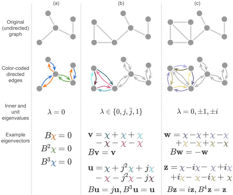
Figure 3.1(a) shows a tree with two layers. Per Proposition 3.1, all its NB-eigenvalues are zero. Per proposition 3.2, the characteristic vectors of the orange edges lie in the kernel of $B$ , while the characteristic vectors of the green and blue edges lie in the kernels of $B^{2}$ and $B^{3}$ , respectively. Per Proposition , we have $GM(0)=3$ and $AM(0)=8$ . Figure 3.1(b) shows a graph with one cycle and non-empty $1$ -shell. Note the $1$ -shell is isomorphic to the graph in (a), and the cycle is a pendant of size $3$ (see Figure 1.2). The $1$ -shell gives rise to the zero eigenvalue, and the composition of the kernels of $B,B^{2},B^{3}$ is similar to that of (a). The pendant gives rise to three new eigenvalues that are all third roots of unity. Example eigenvectors are shown. Figure 3.1(c) shows a graph with two cycles and non-empty $1$ -shell. The $1$ -shell is the same as in (a) and (b), and the cycle is a collar of length $4$ . As before, the $1$ -shell gives rise to the zero eigenvalue and the kernels of $B,B^{2},B^{3}$ . The collar gives rise to eigenvalues that are fourth roots of unity. Example eigenvectors are shown. The multiplicities of the roots of unity in (b) and (c) is given by Theorem 4.6.

Figure 3.2(a) shows the well-known Karate Club graph [21]. Its $1$ -shell is comprised of only one layer with one node (the orange node in the Figure), and therefore $AM(0)=2,GM(0)=1$ . The purple nodes form a collar of size $4$ . Any four of the green nodes that form a cycle form a collar of size $4$ . Note the nodes of degree greater than $2$ in the purple collar are not neighbors, while the nodes of degree greater than $2$ in the green collars are neighbors.

Figure 3.2: (a) The Karate Club graph. See Section 3.4 for discussion. (b) A graph made of two linearly independent and overlapping collars. See Section 4.2.4 for discussion. Note it is a subgraph of the Karate Club graph.

4 Graphs with two cycles or more

In this Section, all graphs have at least two cycles, and we continue to assume minimum md $2$ . We analyze the eigenvalues in order of increasing magnitude, following the categories shown in Figure 1.1. The case $\lambda=0$ has already been dealt with in Section 3.2. We recall well-known results on the impossibility of finding eigenvalues with $0<|\lambda|<1$ in Section 4.1, which completes the characterization of the inner eigenvalues. Next, we treat the unit eigenvalues, $|\lambda|=1$ , case by case in Section 4.2. We then focus on the outer eigenvalues in Section 4.3, where we formulate a conjecture on their simplicity. Finally, we recall known results on leading eigenvalues i.e. those with $|\lambda|=\rho$ .

4.1 The inner eigenvalues

It is a well-known fact that eigenvalues with $0<|\lambda|<1$ are in fact impossible. Kotani and Sunada [13], Theorem 1.3(a), prove this in the language of Zeta functions, by making use of the Ihara-Bass formula (2.3). For completeness, here we paraphrase their theorem in the language of the NB-matrix.

Theorem 4.1 (from [13]).

Let $G$ be a graph with minimum degree at least $2$ with at least two cycles. Then, every NB-eigenvalue $\lambda$ satisfies $1\leq|\lambda|$ . ∎

Remark.

The proof of this Theorem can be found in Section 6 of [13]. It can be read without much background in the theory of graph Zeta functions, by keeping in mind that if $\lambda$ is a NB-eigenvalue then $1/\lambda$ is a pole of (2.3).

4.2 The unit eigenvalues

We give a complete characterization of the unit eigenvalues and their eigenvectors in arbitrary graphs. Some of our arguments require the graph to be md $2$ , as we have been assuming, but Section 3 establishes that nodes of degree $1$ (and in fact any node in the $1$ -shell) have no influence on the unit eigenvalues. Thus, the results here are valid for arbitrary graphs, without restriction. We first prove that all unit eigenvalues must be roots of unity. In this case, there exists a set of nodes $\mathcal{C}$ that is always a pendant, a collar, or a bracelet such that the associated eigenvector $\mathbf{v}$ is supported on $\mathcal{C}$ , i.e. $\mathbf{v}_{k\to l}\neq 0$ if and only if $k,l\in\mathcal{C}$ .

4.2.1 Only roots of unity are NB-eigenvalues

Assume $B\mathbf{v}=\lambda\mathbf{v}$ . By the properties of unitary matrices, $\lambda$ is unitary if and only if $B^{*}B\mathbf{v}=BB^{*}\mathbf{v}=\mathbf{v}$ . Therefore, we start our discussion by computing $B^{*}B$ and $BB^{*}$ . For this purpose, define $\mathchoice{\vec{\mathbf{v}}^{{{l}}}}{\vec{\mathbf{v}}^{{{l}}}}{\vec{\mathbf{v}}^{{{l}}}}{\vec{\mathbf{v}}^{{{l}}}}\coloneqq\sum_{i}a_{il}\mathbf{v}_{i\to l}$ and $\mathchoice{\hphantom{{}^{{{k}}}}\vec{\mathbf{v}}^{{\kern-9.3545pt{k}\kern 6.5382pt}}_{{\kern-6.1493pt\kern 6.5382pt}}}{\hphantom{{}^{{{k}}}}\vec{\mathbf{v}}^{{\kern-9.3545pt{k}\kern 6.5382pt}}_{{\kern-6.1493pt\kern 6.5382pt}}}{\hphantom{{}^{{{k}}}}\vec{\mathbf{v}}^{{\kern-8.58159pt{k}\kern 6.5382pt}}_{{\kern-6.1493pt\kern 6.5382pt}}}{\hphantom{{}^{{{k}}}}\vec{\mathbf{v}}^{{\kern-8.58159pt{k}\kern 6.5382pt}}_{{\kern-6.1493pt\kern 6.5382pt}}}\coloneqq\sum_{i}a_{ik}\mathbf{v}_{k\to i}$ . Recall from Equation (2.5) that if $\mathbf{v}$ is the Perron eigenvector of $B$ , then $\mathchoice{\vec{\mathbf{v}}^{{{k}}}}{\vec{\mathbf{v}}^{{{k}}}}{\vec{\mathbf{v}}^{{{k}}}}{\vec{\mathbf{v}}^{{{k}}}}$ is the NB-centrality of $k$ .

Lemma 4.2.

For any vector $\mathbf{v}$ , the following hold (see Figure 4.1).

	$\displaystyle\left(B^{*}B\mathbf{v}\right)_{k\to l}$	$\displaystyle=\left(d_{l}-2\right)\mathchoice{\vec{\mathbf{v}}^{{{l}}}}{\vec{\mathbf{v}}^{{{l}}}}{\vec{\mathbf{v}}^{{{l}}}}{\vec{\mathbf{v}}^{{{l}}}}+\mathbf{v}_{k\to l}$		(4.1)
	$\displaystyle\left(BB^{*}\mathbf{v}\right)_{k\to l}$	$\displaystyle=\left(d_{k}-2\right)\mathchoice{\hphantom{{}^{{{k}}}}\vec{\mathbf{v}}^{{\kern-9.3545pt{k}\kern 6.5382pt}}_{{\kern-6.1493pt\kern 6.5382pt}}}{\hphantom{{}^{{{k}}}}\vec{\mathbf{v}}^{{\kern-9.3545pt{k}\kern 6.5382pt}}_{{\kern-6.1493pt\kern 6.5382pt}}}{\hphantom{{}^{{{k}}}}\vec{\mathbf{v}}^{{\kern-8.58159pt{k}\kern 6.5382pt}}_{{\kern-6.1493pt\kern 6.5382pt}}}{\hphantom{{}^{{{k}}}}\vec{\mathbf{v}}^{{\kern-8.58159pt{k}\kern 6.5382pt}}_{{\kern-6.1493pt\kern 6.5382pt}}}+\mathbf{v}_{k\to l}.$		(4.2)

Proof.

This is direct from the definition of $B$ . For brevity, we show only the case $B^{*}B\mathbf{v}$ .

	$\displaystyle\left(B^{*}B\mathbf{v}\right)_{k\to l}$	$\displaystyle=\sum_{i\to j}\delta_{il}\left(1-\delta_{jk}\right)\sum_{r\to s}\delta_{is}\left(1-\delta_{jr}\right)\mathbf{v}_{r\to s}$
		$\displaystyle=\sum_{j\neq k}a_{jl}\left(\sum_{r}a_{rl}\mathbf{v}_{r\to l}-\mathbf{v}_{j\to l}\right)$
		$\displaystyle=\left(d_{l}-1\right)\mathchoice{\vec{\mathbf{v}}^{{{l}}}}{\vec{\mathbf{v}}^{{{l}}}}{\vec{\mathbf{v}}^{{{l}}}}{\vec{\mathbf{v}}^{{{l}}}}-\mathchoice{\vec{\mathbf{v}}^{{{l}}}}{\vec{\mathbf{v}}^{{{l}}}}{\vec{\mathbf{v}}^{{{l}}}}{\vec{\mathbf{v}}^{{{l}}}}+\mathbf{v}_{k\to l}.$

∎

Figure 4.1: The action of

B,B^{*},B^{*}B

and

BB^{*}

on a vector

\mathbf{v}

. See Lemma 4.2.

Remark.

Note that $\mathchoice{\hphantom{{}^{{{k}}}}\vec{\mathbf{v}}^{{\kern-9.3545pt{k}\kern 6.5382pt}}_{{\kern-6.1493pt\kern 6.5382pt}}}{\hphantom{{}^{{{k}}}}\vec{\mathbf{v}}^{{\kern-9.3545pt{k}\kern 6.5382pt}}_{{\kern-6.1493pt\kern 6.5382pt}}}{\hphantom{{}^{{{k}}}}\vec{\mathbf{v}}^{{\kern-8.58159pt{k}\kern 6.5382pt}}_{{\kern-6.1493pt\kern 6.5382pt}}}{\hphantom{{}^{{{k}}}}\vec{\mathbf{v}}^{{\kern-8.58159pt{k}\kern 6.5382pt}}_{{\kern-6.1493pt\kern 6.5382pt}}}$ sums over the directed edges that have $k$ as a source, reflected by the use of “ $k\!\to$ ” in the notation. Similarly, $\mathchoice{\vec{\mathbf{v}}^{{{k}}}}{\vec{\mathbf{v}}^{{{k}}}}{\vec{\mathbf{v}}^{{{k}}}}{\vec{\mathbf{v}}^{{{k}}}}$ sums over the directed edges that have $k$ as a target, reflected by the use of “ $\to\!k$ ”. We pronounce $\mathchoice{\hphantom{{}^{{{k}}}}\vec{\mathbf{v}}^{{\kern-9.3545pt{k}\kern 6.5382pt}}_{{\kern-6.1493pt\kern 6.5382pt}}}{\hphantom{{}^{{{k}}}}\vec{\mathbf{v}}^{{\kern-9.3545pt{k}\kern 6.5382pt}}_{{\kern-6.1493pt\kern 6.5382pt}}}{\hphantom{{}^{{{k}}}}\vec{\mathbf{v}}^{{\kern-8.58159pt{k}\kern 6.5382pt}}_{{\kern-6.1493pt\kern 6.5382pt}}}{\hphantom{{}^{{{k}}}}\vec{\mathbf{v}}^{{\kern-8.58159pt{k}\kern 6.5382pt}}_{{\kern-6.1493pt\kern 6.5382pt}}}$ as “ $\mathbf{v}$ from k” and $\mathchoice{\vec{\mathbf{v}}^{{{k}}}}{\vec{\mathbf{v}}^{{{k}}}}{\vec{\mathbf{v}}^{{{k}}}}{\vec{\mathbf{v}}^{{{k}}}}$ as “ $\mathbf{v}$ into $k$ ”.

Example 4.3.

Figure 4.2: The nodes in

\mathcal{D}

induce a cycle. The node

k\in\mathcal{D}

has a neighbor

l\notin\mathcal{D}

. Left: a vector

\mathbf{v}

supported on

\mathcal{D}

. Right: if

\mathbf{v}

is an eigenvector, the sum of all values incoming to

k

must be zero. If

\left(B\mathbf{v}\right)_{k\to l}

is non-zero, we say that

\mathbf{v}

leaks out of

\mathcal{D}

via

k

. Nodes with degree

2

can never leak.

Due to Lemma 4.2, to understand the eigenvectors of unit eigenvalues, it is sufficient to understand those $\mathbf{v}$ that satisfy $\left(d_{k}-2\right)\mathchoice{\hphantom{{}^{{{k}}}}\vec{\mathbf{v}}^{{\kern-9.3545pt{k}\kern 6.5382pt}}_{{\kern-6.1493pt\kern 6.5382pt}}}{\hphantom{{}^{{{k}}}}\vec{\mathbf{v}}^{{\kern-9.3545pt{k}\kern 6.5382pt}}_{{\kern-6.1493pt\kern 6.5382pt}}}{\hphantom{{}^{{{k}}}}\vec{\mathbf{v}}^{{\kern-8.58159pt{k}\kern 6.5382pt}}_{{\kern-6.1493pt\kern 6.5382pt}}}{\hphantom{{}^{{{k}}}}\vec{\mathbf{v}}^{{\kern-8.58159pt{k}\kern 6.5382pt}}_{{\kern-6.1493pt\kern 6.5382pt}}}=\left(d_{l}-2\right)\mathchoice{\vec{\mathbf{v}}^{{{l}}}}{\vec{\mathbf{v}}^{{{l}}}}{\vec{\mathbf{v}}^{{{l}}}}{\vec{\mathbf{v}}^{{{l}}}}=0$ for each pair of neighboring $k,l$ . For this purpose, consider the following situation and the accompanying Figure 4.2. Let $G$ be a graph with NB-matrix $B$ . Let $\mathcal{D}$ be a set of nodes whose induced subgraph is a cycle. Suppose $B\mathbf{v}=\lambda\mathbf{v}$ with $\lambda\neq 0$ and that $\mathbf{v}$ is supported on $\mathcal{D}$ . Let $k\in\text{$\mathcal{D}$},l\notin\mathcal{D}$ be neighbors. Since $\mathbf{v}$ is an eigenvector supported on $\mathcal{D}$ , we have

0=\lambda\mathbf{v}_{k\to l}=\left(B\mathbf{v}\right)_{k\to l}=\sum_{i}a_{ik}\mathbf{v}_{i\to k}-\mathbf{v}_{l\to k}=\mathchoice{\vec{\mathbf{v}}^{{{k}}}}{\vec{\mathbf{v}}^{{{k}}}}{\vec{\mathbf{v}}^{{{k}}}}{\vec{\mathbf{v}}^{{{k}}}},

(4.3)

where the last equality uses the fact that $\mathbf{v}_{l\to k}=0$ . Thus, a necessary condition for $\mathbf{v}$ to be an eigenvector supported on a cycle $\mathcal{D}$ is that for every $k\in\mathcal{D}$ with a neighbor outside of $\mathcal{D}$ , we must have $\mathchoice{\vec{\mathbf{v}}^{{{k}}}}{\vec{\mathbf{v}}^{{{k}}}}{\vec{\mathbf{v}}^{{{k}}}}{\vec{\mathbf{v}}^{{{k}}}}=0$ . Note that if $k\in\mathcal{D}$ has no neighbors outside of $\mathcal{D}$ , i.e. if its degree is $2$ , then there is no restriction on $\mathchoice{\vec{\mathbf{v}}^{{{k}}}}{\vec{\mathbf{v}}^{{{k}}}}{\vec{\mathbf{v}}^{{{k}}}}{\vec{\mathbf{v}}^{{{k}}}}$ . In other words, $\mathbf{v}$ satisfies $\left(d_{k}-2\right)\mathchoice{\vec{\mathbf{v}}^{{{k}}}}{\vec{\mathbf{v}}^{{{k}}}}{\vec{\mathbf{v}}^{{{k}}}}{\vec{\mathbf{v}}^{{{k}}}}=0$ for each $k$ , and therefore $B^{*}B\mathbf{v}=\mathbf{v}$ by Lemma 4.2. Furthermore, we have $BB^{*}\mathbf{v}=\mathbf{v}$ as well, by Lemma C.1. Lastly, if $r$ is the length of the cycle induced by $\mathcal{D}$ , we have $B^{r}\mathbf{v}=\mathbf{v}$ and thus $\lambda^{r}=1$ .

Before moving forward, let us capture the property $\left(d_{k}-2\right)\mathchoice{\vec{\mathbf{v}}^{{{k}}}}{\vec{\mathbf{v}}^{{{k}}}}{\vec{\mathbf{v}}^{{{k}}}}{\vec{\mathbf{v}}^{{{k}}}}=0$ with the following terminology, inspired by Example 4.2.

Definition 4.4.

Consider a vector $\mathbf{v}$ (not necessarily an eigenvector) with support $\mathcal{D}$ (not necessarily a cycle). If there is a $k\in\mathcal{D}$ such that $\left(d_{k}-2\right)\mathchoice{\vec{\mathbf{v}}^{{{k}}}}{\vec{\mathbf{v}}^{{{k}}}}{\vec{\mathbf{v}}^{{{k}}}}{\vec{\mathbf{v}}^{{{k}}}}\neq 0$ , we say that $\mathbf{v}$ leaks out of $\mathcal{D}$ via $k$ , or simply that $\mathbf{v}$ is leaky. If $\mathbf{v}$ does not leak via any node, we say that $\mathbf{v}$ is non-leaky. See Figure 4.2.

Example 4.2 shows that if $\mathbf{v}$ is an eigenvector supported on a cycle, then $\mathbf{v}$ must be non-leaky and its corresponding eigenvalue must be a root of unity. The following theorem is essentially a generalization of this observation.

Theorem 4.5.

Suppose $B\mathbf{v}=\lambda\mathbf{v}$ with $\lambda\neq 0$ . $\mathbf{v}$ is non-leaky if and only if $\lambda$ is a root of unity.

Proof.

If $\lambda$ is a root of unity then it is unitary; by Lemma C.2, $\mathbf{v}$ is non-leaky. Now assume $\mathbf{v}$ is non-leaky and let $\mathcal{D}$ be the support of $\mathbf{v}$ . We proceed in two cases.

1.

Assume that $\mathcal{D}$ contains no nodes of degree $2$ and take two neighbors $k,l$ with $\mathbf{v}_{k\to l}\neq 0$ . Since $\mathbf{v}$ is non-leaky, we must have $\mathchoice{\vec{\mathbf{v}}^{{{k}}}}{\vec{\mathbf{v}}^{{{k}}}}{\vec{\mathbf{v}}^{{{k}}}}{\vec{\mathbf{v}}^{{{k}}}}=\mathchoice{\vec{\mathbf{v}}^{{{l}}}}{\vec{\mathbf{v}}^{{{l}}}}{\vec{\mathbf{v}}^{{{l}}}}{\vec{\mathbf{v}}^{{{l}}}}=0$ . By Equation (2.4) this is equivalent to $\lambda\mathbf{v}_{k\to l}+\mathbf{v}_{l\to k}=0=\lambda\mathbf{v}_{l\to k}+\mathbf{v}_{k\to l}$ . Multiply the first equation by $\lambda$ and replace in the second equation to obtain $0=\left(\lambda^{2}-1\right)\mathbf{v}_{k\to l}.$ Therefore, $\lambda$ must be a square root of unity.
2.

Assume that $k\in\mathcal{D}$ has degree $2$ . We will show there exists a vector $\mathbf{c}$ such that $B\mathbf{c}=\lambda\mathbf{c}$ and $\mathbf{c}$ is non-leaky and supported on a cycle. In that case, $\lambda$ must be a root of unity by Example 4.2. Let $i,l\in\mathcal{D}$ be the two neighbors of $k$ , and note that $\lambda\text{$\mathbf{v}$}_{k\to l}=\mathbf{v}_{i\to k}$ . Take a $\mathcal{C}\subset\mathcal{D}$ such that $i,k,l\in\mathcal{C}$ and the graph induced by $\mathcal{C}$ is a cycle. This is always possible due to Lemma C.3. Suppose $\mathcal{C}$ contains $r$ nodes and label them by consecutive numbers $k=1,l=2,\ldots,i=r$ . Define $\mathbf{c}_{i\to k}\coloneqq\mathbf{v}_{i\to k}$ and $\mathbf{c}_{k\to l}\coloneqq\mathbf{v}_{k\to l}$ . Define all other edges as $\mathbf{c}_{j\to(j+1)}\coloneqq\lambda\mathbf{c}_{(j-1)\to j},\,j=2,\ldots,r-1$ . By construction, $\mathbf{c}$ is non-leaky and supported on a cycle; by Example (4.2) it must be an eigenvector with eigenvalue $\lambda$ . Therefore, $\lambda^{r}=1$ .

∎

Theorem 4.6.

$\lambda$ is not defective, i.e. $AM(\lambda)=GM(\lambda)$ .

Proof.

We show that any generalized eigenvector must be an eigenvector. Let $\mathbf{c}$ be such that $\left(B-\lambda I\right)^{2}\mathbf{c}=0$ , and define $\mathbf{v}\coloneqq\left(B-\lambda I\right)\mathbf{c}$ . Note that $\mathbf{v}$ is an eigenvector of eigenvalue $\lambda$ (or it is the zero vector). We first prove that $\mathbf{c}$ must be non-leaky; we proceed in three cases. First, if $\mathbf{v}_{k\to l}$ equals $0$ , we have $\left(B\mathbf{c}\right)_{k\to l}=\lambda\mathbf{c}_{k\to l}$ . That is, $\mathbf{c}$ behaves like an eigenvector outside the support of $\mathbf{v}$ . In particular, $\left(d_{k}-2\right)\mathchoice{\hphantom{{}^{{{k}}}}\vec{\mathbf{c}}^{{\kern-9.3545pt{k}\kern 6.5382pt}}_{{\kern-6.1493pt\kern 6.5382pt}}}{\hphantom{{}^{{{k}}}}\vec{\mathbf{c}}^{{\kern-9.3545pt{k}\kern 6.5382pt}}_{{\kern-6.1493pt\kern 6.5382pt}}}{\hphantom{{}^{{{k}}}}\vec{\mathbf{c}}^{{\kern-8.58159pt{k}\kern 6.5382pt}}_{{\kern-6.1493pt\kern 6.5382pt}}}{\hphantom{{}^{{{k}}}}\vec{\mathbf{c}}^{{\kern-8.58159pt{k}\kern 6.5382pt}}_{{\kern-6.1493pt\kern 6.5382pt}}}$ = 0 for any $k$ not in the support of $\mathbf{v}$ . Second, for any node $k$ of degree $2$ , we have ${\left(d_{k}-2\right)\mathchoice{\hphantom{{}^{{{k}}}}\vec{\mathbf{c}}^{{\kern-9.3545pt{k}\kern 6.5382pt}}_{{\kern-6.1493pt\kern 6.5382pt}}}{\hphantom{{}^{{{k}}}}\vec{\mathbf{c}}^{{\kern-9.3545pt{k}\kern 6.5382pt}}_{{\kern-6.1493pt\kern 6.5382pt}}}{\hphantom{{}^{{{k}}}}\vec{\mathbf{c}}^{{\kern-8.58159pt{k}\kern 6.5382pt}}_{{\kern-6.1493pt\kern 6.5382pt}}}{\hphantom{{}^{{{k}}}}\vec{\mathbf{c}}^{{\kern-8.58159pt{k}\kern 6.5382pt}}_{{\kern-6.1493pt\kern 6.5382pt}}}=0}$ , regardless of whether or not $k$ is in the support of $\mathbf{v}$ .

Third, let $k$ be in the support of $\mathbf{v}$ with $d_{k}>2$ and thus $\mathchoice{\hphantom{{}^{{{k}}}}\vec{\mathbf{v}}^{{\kern-9.3545pt{k}\kern 6.5382pt}}_{{\kern-6.1493pt\kern 6.5382pt}}}{\hphantom{{}^{{{k}}}}\vec{\mathbf{v}}^{{\kern-9.3545pt{k}\kern 6.5382pt}}_{{\kern-6.1493pt\kern 6.5382pt}}}{\hphantom{{}^{{{k}}}}\vec{\mathbf{v}}^{{\kern-8.58159pt{k}\kern 6.5382pt}}_{{\kern-6.1493pt\kern 6.5382pt}}}{\hphantom{{}^{{{k}}}}\vec{\mathbf{v}}^{{\kern-8.58159pt{k}\kern 6.5382pt}}_{{\kern-6.1493pt\kern 6.5382pt}}}=0$ . Using the definition $\mathbf{v}_{k\to l}={\mathchoice{\hphantom{{}^{{{k}}}}\vec{\mathbf{c}}^{{\kern-9.3545pt{k}\kern 6.5382pt}}_{{\kern-6.1493pt\kern 6.5382pt}}}{\hphantom{{}^{{{k}}}}\vec{\mathbf{c}}^{{\kern-9.3545pt{k}\kern 6.5382pt}}_{{\kern-6.1493pt\kern 6.5382pt}}}{\hphantom{{}^{{{k}}}}\vec{\mathbf{c}}^{{\kern-8.58159pt{k}\kern 6.5382pt}}_{{\kern-6.1493pt\kern 6.5382pt}}}{\hphantom{{}^{{{k}}}}\vec{\mathbf{c}}^{{\kern-8.58159pt{k}\kern 6.5382pt}}_{{\kern-6.1493pt\kern 6.5382pt}}}}-\mathbf{c}_{l\to k}-\lambda\,\mathbf{c}_{k\to l}$ and summing over every neighbor $l$ of $k$ , we obtain $\lambda{\mathchoice{\hphantom{{}^{{{k}}}}\vec{\mathbf{c}}^{{\kern-9.3545pt{k}\kern 6.5382pt}}_{{\kern-6.1493pt\kern 6.5382pt}}}{\hphantom{{}^{{{k}}}}\vec{\mathbf{c}}^{{\kern-9.3545pt{k}\kern 6.5382pt}}_{{\kern-6.1493pt\kern 6.5382pt}}}{\hphantom{{}^{{{k}}}}\vec{\mathbf{c}}^{{\kern-8.58159pt{k}\kern 6.5382pt}}_{{\kern-6.1493pt\kern 6.5382pt}}}{\hphantom{{}^{{{k}}}}\vec{\mathbf{c}}^{{\kern-8.58159pt{k}\kern 6.5382pt}}_{{\kern-6.1493pt\kern 6.5382pt}}}}=\left(d_{k}-1\right){\mathchoice{\vec{\mathbf{c}}^{{{k}}}}{\vec{\mathbf{c}}^{{{k}}}}{\vec{\mathbf{c}}^{{{k}}}}{\vec{\mathbf{c}}^{{{k}}}}}$ , or equivalently

\lambda{\mathchoice{\hphantom{{}^{{{k}}}}\vec{\mathbf{c}}^{{\kern-9.3545pt{k}\kern 6.5382pt}}_{{\kern-6.1493pt\kern 6.5382pt}}}{\hphantom{{}^{{{k}}}}\vec{\mathbf{c}}^{{\kern-9.3545pt{k}\kern 6.5382pt}}_{{\kern-6.1493pt\kern 6.5382pt}}}{\hphantom{{}^{{{k}}}}\vec{\mathbf{c}}^{{\kern-8.58159pt{k}\kern 6.5382pt}}_{{\kern-6.1493pt\kern 6.5382pt}}}{\hphantom{{}^{{{k}}}}\vec{\mathbf{c}}^{{\kern-8.58159pt{k}\kern 6.5382pt}}_{{\kern-6.1493pt\kern 6.5382pt}}}}-{\mathchoice{\vec{\mathbf{c}}^{{{k}}}}{\vec{\mathbf{c}}^{{{k}}}}{\vec{\mathbf{c}}^{{{k}}}}{\vec{\mathbf{c}}^{{{k}}}}}=\left(d_{k}-2\right){\mathchoice{\vec{\mathbf{c}}^{{{k}}}}{\vec{\mathbf{c}}^{{{k}}}}{\vec{\mathbf{c}}^{{{k}}}}{\vec{\mathbf{c}}^{{{k}}}}}.

(4.4)

In the following, we show that $\mathbf{c}$ does not leak via $k$ by showing that the two members of this last equation in fact equal zero. We proceed in two sub-cases.

Assume $\lambda^{2}=1$ . Let $l$ be a node outside the support of $\mathbf{v}$ , i.e. $\mathbf{c}$ behaves like an eigenvector on $k\to l$ and

\lambda\mathbf{c}_{k\to l}=\left(B\mathbf{c}\right)_{k\to l}={\mathchoice{\vec{\mathbf{c}}^{{{k}}}}{\vec{\mathbf{c}}^{{{k}}}}{\vec{\mathbf{c}}^{{{k}}}}{\vec{\mathbf{c}}^{{{k}}}}}-\mathbf{c}_{l\to k}=\sum_{l\in supp(\mathbf{v})}\mathbf{c}_{l\to k}+\sum_{l\notin supp(\mathbf{v})}\mathbf{c}_{l\to k}-\mathbf{c}_{l\to k}.

Note that $\sum_{l\notin supp(\mathbf{v})}\mathbf{c}_{l\to k}=0$ since $\mathbf{c}$ is an eigenvector outside of the support of $\mathbf{v}$ and therefore it does not leak through $k$ . Therefore $\lambda\mathbf{c}_{k\to l}=\sum_{l\in supp(\mathbf{v})}\mathbf{c}_{l\to k}-\mathbf{c}_{l\to k}$ . On the other hand, we have $\mathbf{c}_{k\to l}+\lambda\mathbf{c}_{l\to k}={\mathchoice{\vec{\mathbf{c}}^{{{l}}}}{\vec{\mathbf{c}}^{{{l}}}}{\vec{\mathbf{c}}^{{{l}}}}{\vec{\mathbf{c}}^{{{l}}}}}=0$ , since $\mathbf{c}$ does not leak through $l$ . These two equations simplify to

\sum_{l\in supp(\mathbf{v})}\mathbf{c}_{l\to k}=\left(1-\lambda^{2}\right)\mathbf{c}_{l\to k}=0.

All together, we have

{\mathchoice{\vec{\mathbf{c}}^{{{k}}}}{\vec{\mathbf{c}}^{{{k}}}}{\vec{\mathbf{c}}^{{{k}}}}{\vec{\mathbf{c}}^{{{k}}}}}=\sum_{l\in supp(\mathbf{v})}\mathbf{c}_{l\to k}+\sum_{l\notin supp(\mathbf{v})}\mathbf{c}_{l\to k}=0+0=0,

and Equation (4.4) equals zero, as desired.

Assume $\lambda^{r}=1$ , with $r\neq 2$ . To fix ideas, assume that $\mathbf{v}$ is supported on a single cycle. In this case, $k$ has exactly two neighbors in the support of $\mathbf{v}$ , call them $i$ and $j$ . Since $\mathbf{v}$ is non-leaky, we have

	$\displaystyle\mathchoice{\hphantom{{}^{{{k}}}}\vec{\mathbf{v}}^{{\kern-9.3545pt{k}\kern 6.5382pt}}_{{\kern-6.1493pt\kern 6.5382pt}}}{\hphantom{{}^{{{k}}}}\vec{\mathbf{v}}^{{\kern-9.3545pt{k}\kern 6.5382pt}}_{{\kern-6.1493pt\kern 6.5382pt}}}{\hphantom{{}^{{{k}}}}\vec{\mathbf{v}}^{{\kern-8.58159pt{k}\kern 6.5382pt}}_{{\kern-6.1493pt\kern 6.5382pt}}}{\hphantom{{}^{{{k}}}}\vec{\mathbf{v}}^{{\kern-8.58159pt{k}\kern 6.5382pt}}_{{\kern-6.1493pt\kern 6.5382pt}}}$	$\displaystyle=0$
	$\displaystyle\mathbf{v}_{k\to j}+\mathbf{v}_{k\to i}$	$\displaystyle=0$
	$\displaystyle{\mathchoice{\vec{\mathbf{c}}^{{{k}}}}{\vec{\mathbf{c}}^{{{k}}}}{\vec{\mathbf{c}}^{{{k}}}}{\vec{\mathbf{c}}^{{{k}}}}}-\mathbf{c}_{j\to k}-\lambda\mathbf{c}_{k\to j}+{\mathchoice{\vec{\mathbf{c}}^{{{k}}}}{\vec{\mathbf{c}}^{{{k}}}}{\vec{\mathbf{c}}^{{{k}}}}{\vec{\mathbf{c}}^{{{k}}}}}-\mathbf{c}_{i\to k}-\lambda\mathbf{c}_{k\to i}$	$\displaystyle=0$
	$\displaystyle\sum_{l\notin supp(\mathbf{v})}\mathbf{c}_{l\to k}+\mathbf{c}_{i\to k}+\sum_{l\notin supp(\mathbf{v})}\mathbf{c}_{l\to k}+\mathbf{c}_{j\to k}$	$\displaystyle=\lambda\left(\mathbf{c}_{k\to i}+\mathbf{c}_{k\to j}\right)$
	$\displaystyle\mathbf{c}_{i\to k}+\mathbf{c}_{j\to k}$	$\displaystyle=\lambda\left(\mathbf{c}_{k\to i}+\mathbf{c}_{k\to j}\right)$
	$\displaystyle\mathbf{c}_{i\to k}+\mathbf{c}_{j\to k}+\sum_{l\notin supp(\mathbf{v})}\mathbf{c}_{l\to k}$	$\displaystyle=\lambda\left(\mathbf{c}_{k\to i}+\mathbf{c}_{k\to j}+\sum_{l\notin supp(\mathbf{v})}\mathbf{c}_{k\to l}\right)$
	$\displaystyle{\mathchoice{\vec{\mathbf{c}}^{{{k}}}}{\vec{\mathbf{c}}^{{{k}}}}{\vec{\mathbf{c}}^{{{k}}}}{\vec{\mathbf{c}}^{{{k}}}}}$	$\displaystyle=\lambda{\mathchoice{\hphantom{{}^{{{k}}}}\vec{\mathbf{c}}^{{\kern-9.3545pt{k}\kern 6.5382pt}}_{{\kern-6.1493pt\kern 6.5382pt}}}{\hphantom{{}^{{{k}}}}\vec{\mathbf{c}}^{{\kern-9.3545pt{k}\kern 6.5382pt}}_{{\kern-6.1493pt\kern 6.5382pt}}}{\hphantom{{}^{{{k}}}}\vec{\mathbf{c}}^{{\kern-8.58159pt{k}\kern 6.5382pt}}_{{\kern-6.1493pt\kern 6.5382pt}}}{\hphantom{{}^{{{k}}}}\vec{\mathbf{c}}^{{\kern-8.58159pt{k}\kern 6.5382pt}}_{{\kern-6.1493pt\kern 6.5382pt}}}},$

where we have used that $\sum_{l\notin supp(\mathbf{v})}\mathbf{c}_{l\to k}=\sum_{l\notin supp(\mathbf{v})}\mathbf{c}_{k\to l}=0$ . This shows that Equation (4.4) equals zero. The general case when $\mathbf{v}$ is not supported on a single cycle is similar but taking into consideration that $k$ has exactly two neighbors in each of the cycles on which $\mathbf{v}$ is supported.

We have established that $\mathbf{c}$ is non-leaky. Now write $\mathbf{c}=\mathbf{c}^{\prime}+\mathbf{c}^{\prime\prime}$ , where $\mathbf{c}^{\prime}$ is supported on the same support as $\mathbf{v}$ , and $\mathbf{c}^{\prime\prime}$ is supported outside of it. As per our previous observation, $\mathbf{c}^{\prime\prime}$ is an eigenvector of eigenvalue $\lambda$ and therefore it is non-leaky. Since $\mathbf{c}$ is also non-leaky, $\mathbf{c}^{\prime}$ must be non-leaky as well. Per Lemma C.4, $\mathbf{c}^{\prime}$ must be the linear combination of eigenvectors. All of these must correspond to the same eigenvalue $\lambda$ as otherwise, $\mathbf{v}$ would not be in the kernel of $\left(B-\lambda I\right)$ . We have proved that both $\mathbf{c}^{\prime}$ and $\mathbf{c}^{\prime\prime}$ are eigenvectors of $\lambda$ , and thus $\mathbf{c}$ is as well and $\mathbf{v}$ was the zero vector all along. ∎

We have proved that the only numbers on the unit circle that may be NB-eigenvalues are the roots of unity, and when they are, they are never defective. We proceed to compute the exact multiplicity of the complex roots of unity and real roots of unity in turn.

4.2.2 Complex roots of unity

Theorem 4.5 shows that, in graphs with no nodes of degree $2$ , only $\pm 1$ may be unit NB-eigenvalues. In graphs that do have complex roots of unity, we have the following characterization. In this section, we fix a nonzero $\lambda$ and let $B\mathbf{v}=\lambda\mathbf{v}$ with $\lambda^{r}=1$ but $\lambda^{2}\neq 1$ .

Proposition 4.7.

$\mathbf{v}$ can we written as $\mathbf{v}=\sum_{i=1}^{t}\mathbf{c}^{i}$ , where each $\mathbf{c}^{i}$ is an eigenvector supported on a different cycle.

Proof.

With the notations used in Theorem 4.5, put $\mathbf{v}^{0}\coloneqq\mathbf{v}$ and $\mathbf{c}^{1}\coloneqq\mathbf{c}$ . Define $\mathbf{v}^{1}\coloneqq\mathbf{v}^{0}-\mathbf{c}^{1}$ . Since both $\mathbf{v}^{0}$ and $\mathbf{c}^{1}$ are non-leaky eigenvectors, $\mathbf{v}^{1}$ is a non-leaky eigenvector as well. Let $\mathcal{D}_{1}$ be the support of $\mathbf{v}^{1}$ . By construction, we have $\mathbf{v}_{i\to k}^{1}=\mathbf{v}_{k\to l}^{1}=0$ and therefore $k\notin\mathcal{D}_{1}$ . But since $\lambda^{2}\neq 1$ , there must be a $k_{2}\in\mathcal{D}_{1}$ with degree $2$ . Thus we can construct another $\mathbf{c}^{2}$ supported on a cycle containing $k_{2}$ and define $\mathbf{v}^{2}\coloneqq\mathbf{v}^{1}-\mathbf{c}^{2}$ . Note that the support of $\mathbf{v}^{2}$ is a proper subset of $\mathcal{D}_{1}$ as it does not contain $k_{2}$ . We can iterate this construction for $t$ steps until support $\mathbf{v}^{t}$ is supported on a single cycle, i.e. until $\mathbf{v}^{t}=\mathbf{c}^{t}$ . ∎

Proposition 4.8.

Let $\mathcal{C}$ be a set of $r$ nodes that induce either a cycle or a figure eight graph, and suppose $\lambda^{r}=1$ but $\lambda^{2}\neq 1$ . Assume there exists an eigenvector supported on the edges in the graph induced by $\mathcal{C}$ . Then there is only one such eigenvector, up to a scalar.

Proof.

Let $B\mathbf{v}=\lambda\mathbf{v}$ , where $\mathbf{v}$ is nonzero within the graph induced by $\mathcal{C}$ and zero outside of it, and thus $\mathbf{v}$ has $2r$ nonzero coordinates. It is sufficient to show that the condition of being a non-leaky eigenvector supported on $\mathcal{C}$ determines a system of $2r-1$ equations. Label the nodes of $\mathcal{C}$ by $0,2,\ldots,r-1$ such that the node $i$ is adjacent to the nodes labeled $i-1$ and $i+1$ ; here labels are taken $\mod r$ . Since $\mathbf{v}$ is an eigenvector, we have $\mathbf{v}_{i\to(i+1)}=\lambda\mathbf{v}_{(i-1)\to i}$ and $\mathbf{v}_{\left(i+1\right)\to i}=\lambda\mathbf{v}_{i\to\left(i-1\right)}$ for each $i$ ; this gives $2r-2$ independent equations. Without loss of generality we may assume that the node with label $0$ has degree greater than $2$ . Since $\mathbf{v}$ does not leak through the node with label $0$ , we have $0=\mathchoice{\vec{\mathbf{v}}^{{{0}}}}{\vec{\mathbf{v}}^{{{0}}}}{\vec{\mathbf{v}}^{{{0}}}}{\vec{\mathbf{v}}^{{{0}}}}=\mathbf{v}_{r-1\to 0}+\mathbf{v}_{1\to 0}$ , which is an equation independent of the others, for a total of $2r-1$ equations, completing the proof. (Note that in a cycle graph, the condition of non-leakiness is trivial as all nodes have degree $2$ . In that case, we only have a system with $2r-2$ equations, whence the geometric multiplicity of $\lambda$ is $2$ ; cf. Section 3.3.) ∎

Proposition 4.9.

If $r$ is odd, $\mathcal{C}$ must be a pendant. If $r$ is even, $\mathcal{C}$ must be a collar or a bracelet.

Proof.

Suppose the node with label $0$ has degree larger than $2$ and suppose $\mathbf{v}_{r-1\to 0}=1$ , which fixes all other coordinates to be $\mathbf{v}_{i\to\left(i+1\right)}=\lambda^{-i}$ and $\mathbf{v}_{\left(i+1\right)\to i}=-\lambda^{r+1-i}$ . It suffices to inspect $\mathchoice{\vec{\mathbf{v}}^{{{i}}}}{\vec{\mathbf{v}}^{{{i}}}}{\vec{\mathbf{v}}^{{{i}}}}{\vec{\mathbf{v}}^{{{i}}}}=\mathbf{v}_{\left(i-1\right)\to i}+\mathbf{v}_{\left(i+1\right)\to i}=\lambda^{-\left(i-1\right)}-\lambda^{r+1-i}$ for each $i$ ; if $\mathchoice{\vec{\mathbf{v}}^{{{i}}}}{\vec{\mathbf{v}}^{{{i}}}}{\vec{\mathbf{v}}^{{{i}}}}{\vec{\mathbf{v}}^{{{i}}}}\neq 0$ then $i$ must have degree $2$ . The properties of sums of roots of unity are well-known. In particular, if $r$ is odd, $\mathchoice{\vec{\mathbf{v}}^{{{i}}}}{\vec{\mathbf{v}}^{{{i}}}}{\vec{\mathbf{v}}^{{{i}}}}{\vec{\mathbf{v}}^{{{i}}}}$ is zero only when $i=0$ . In other words, only the node with label $0$ can have degree greater than $2$ , which means that $\mathcal{C}$ is a pendant. If $r$ is even, $\mathchoice{\vec{\mathbf{v}}^{{{i}}}}{\vec{\mathbf{v}}^{{{i}}}}{\vec{\mathbf{v}}^{{{i}}}}{\vec{\mathbf{v}}^{{{i}}}}$ is zero only when $i=0$ or $i=r/2$ . In this case, and if $\mathcal{C}$ induces a cycle, then it is a collar; if it induces a figure eight graph (and the nodes $0$ and $r/2$ are actually the same), it is a bracelet. ∎

Corollary 4.10.

$GM(\lambda)$ equals the number of pendants or collars or bracelets of length $r$ . Equivalently, the eigenspace corresponding to $\lambda$ has a basis $\{\mathbf{c}^{i}\}_{i=1}^{t}$ such that the support of each $\mathbf{c}^{i}$ is a pendant or a collar or a bracelet. ∎

4.2.3 Real roots of unity

We proceed to find the algebraic and geometric multiplicity of $\lambda=\pm 1$ . Theorem (4.6) establishes that these quantities are equal, though we present different proofs for each. The proofs for computing the algebraic multiplicity are related to the Ihara-Bass formula of Equation (2.3), while the proofs for computing the geometric multiplicities yield a basis for the corresponding eigenspace similar to that exhibited for complex roots of unity in Corollary 4.10; see Corollary 4.16.

A graph $G$ has at least two cycles if and only if it has more edges than nodes: $m>n$ . In this case, the Ihara-Bass formula (2.3) immediately implies that $AM(\pm 1)\geq m-n$ . For this Section, recall that $D-A$ is called the Laplacian matrix of $G$ , which is always singular, and whose rank is $n-1$ if and only if the graph is connected. An argument closely related to the following proof can be found in [16, 10], though we have arrived at it independently.

Proposition 4.11.

Let $G$ have at least two cycles, i.e. $m>n$ . Then $AM(1)=m-n+1$ .

Proof.

Define $f(u)\coloneqq\det\left(I-uA+u^{2}(D-I)\right)$ and observe that $f(1)=\det\left(D-A\right)=0$ . Therefore, $f(u)=(u-1)g(u)$ and the Ihara-Bass formula (2.3) implies $AM(1)\geq m-n+1$ . Showing $g(1)\neq 0$ finishes the proof. First, note that $g(1)$ equals $f^{\prime}(1)$ . The so-called Jacobi formula shows $f^{\prime}(1)=\Tr\left(\adj\left(D-A\right)\left(D-A+D-2I\right)\right)$ (see [17], Equation (41)). Further, well-known properties of the adjugate show that $\adj\left(D-A\right)=\eta\mathbf{1}\mathbf{1}^{T}$ for some nonzero $\eta$ (see [11], Section 0.8.2 and [15]). All together, we have

$\displaystyle g(1)=f^{\prime}(1)$	$\displaystyle=\Tr\left(\adj\left(D-A\right)\left(D-A+D-2I\right)\right)$	(4.5)
	$\displaystyle=\eta\Tr\left(\mathbf{1}\mathbf{1}^{T}\left(D-A\right)+\mathbf{11}^{T}\left(D-2I\right)\right)$
	$\displaystyle=\eta\mathbf{1}^{T}\left(D-A\right)\mathbf{1}+\eta\mathbf{1}^{T}\left(D-2I\right)\mathbf{1}$
	$\displaystyle=\eta\left(2m-2n\right)\neq 0,$	(4.6)

where the third line uses Lemma C.5. ∎

Proposition 4.12.

Let $G$ have at least two cycles. Then $GM(1)=m-n+1$ .

Proof.

Since $GM$ is bounded above by $AM$ , we have $GM(1)\leq m-n+1$ . Thus we only need to show that there exists a set of $m-n+1$ linearly independent vectors that satisfy $B\mathbf{v}=\mathbf{v}$ . Inspection of (2.4) when $\lambda=1$ shows that there exists a global constant $q$ such that

\mathbf{v}_{k\to l}+\mathbf{v}_{l\to k}=q=\mathchoice{\vec{\mathbf{v}}^{{{l}}}}{\vec{\mathbf{v}}^{{{l}}}}{\vec{\mathbf{v}}^{{{l}}}}{\vec{\mathbf{v}}^{{{l}}}}

for any neighboring nodes $k,l$ . Summing the left equation for each edge yields

\frac{1}{2}\sum_{k,l}a_{kl}\left(\mathbf{v}_{k\to l}+\mathbf{v}_{l\to k}\right)=mq,

while summing the right equation for each of the $n$ nodes yields

nq=\sum_{l}\mathchoice{\vec{\mathbf{v}}^{{{l}}}}{\vec{\mathbf{v}}^{{{l}}}}{\vec{\mathbf{v}}^{{{l}}}}{\vec{\mathbf{v}}^{{{l}}}}.

Note these two equations sum each of the coordinates of $\mathbf{v}$ exactly once; thus $nq=mq$ and $q=0$ . We conclude that $\mathbf{v}$ satisfies the system

\begin{cases}\mathchoice{\vec{\mathbf{v}}^{{{l}}}}{\vec{\mathbf{v}}^{{{l}}}}{\vec{\mathbf{v}}^{{{l}}}}{\vec{\mathbf{v}}^{{{l}}}}=0&\text{for each node }l,\\ \mathbf{v}_{k\to l}+\mathbf{v}_{l\to k}=0&\text{for each edge }k-l.\end{cases}

(4.7)

Now take a spanning tree $T$ of $G$ and an edge $u_{0}-v_{0}$ not in $T$ . The edge $u_{0}-v_{0}$ determines a unique NB-cycle $c$ all of whose edges are in $T$ except for $u_{0}-v_{0}$ . Choose an arbitrary orientation for the cycle, say $c=u_{0}\to v_{0},u_{1}\to v_{1},\ldots,u_{r}\to v_{r}=u_{0}$ and consider the vector $\mathbf{v}^{u_{0}\to v_{0}}\coloneqq\sum_{i=0}^{r}\chi^{u_{i}\to v_{i}}-\chi^{v_{i}\to u_{i}}$ . It can be manually checked that $\mathbf{v}$ satisfies (4.7). (See Figure 3.1(b) for an example.) Now, for each $\left(k-l\right)\notin T$ , define $\mathbf{v}^{k\to l}$ similarly to $\mathbf{v}^{u_{0}\to v_{0}}$ above. The set $\{\mathbf{v}^{k\to l}:\left(k-l\right)\notin T\}$ is linearly independent since each vector $\mathbf{v}^{k\to l}$ has a non-zero entry at coordinate $k\to l$ , and all other vectors are zero at that coordinate. Since there are exactly $m-n+1$ edges not in $T$ , we have proved $GM(1)\geq m-n+1$ . ∎

Corollary 4.13.

$GM(1)$ is the number of linearly independent ways there are to assign current flows to a graph in such a way that they satisfy Kirchoff’s law of circuits.

Proof.

If we interpret $G$ as an electrical circuit and the coordinate $\mathbf{v}_{k\to l}$ as the current flow in the direction of $k$ toward $l$ , then (4.7) is exactly equivalent to Kirchoff’s law. ∎

For our treatment of $\lambda=-1$ , recall that $D+A$ is called the signless Laplacian of $G$ . The proofs of the two following propositions are similar to those of Propositions 4.11 and 4.12.

Proposition 4.14.

Let $G$ have at least two cycles. Then $AM(-1)=m-n+1$ if $G$ is bipartite and $AM(-1)=m-n$ if $G$ is not bipartite.

Proof.

Define $f(u)$ as in Proposition 4.11 and observe that $f(-1)=\det\left(D+A\right)$ , where $D+A$ is called the signless Laplacian of $G$ . It is known that $D+A$ is singular if and only if $G$ is bipartite [4]. Therefore, if $G$ is not bipartite, $f(-1)\neq 0$ and $AM(-1)=m-n$ due to the Ihara-Bass formula (2.3). If $G$ is bipartite, $f(-1)=0$ and $AM(-1)\geq m-n+1$ . In this case, write $f(u)=(1+u)g(u)$ and note $f^{\prime}(-1)=g(-1)$ . To finish, we show $g(-1)\neq 0$ . Let the partition of the node set be $U_{1}$ and $U_{2}$ and define the vector $\mathbf{v}$ by putting $\mathbf{v}_{i}=1$ if $i\in U_{1}$ and $\mathbf{v}_{j}=-1$ if $j\in U_{2}$ . A similar procedure as in Proposition 4.11 shows that

g(-1)=f^{\prime}(-1)=\Tr\left(\adj\left(D+A\right)\left(2I-D\right)\right)=\mathbf{v}^{T}\left(2I-D\right)\mathbf{v}=\eta\left(2n-2m\right)\neq 0,

for some nonzero number $\eta$ . ∎

Proposition 4.15.

Let $G$ have at least two cycles. Then $GM(-1)=m-n+1$ if $G$ is bipartite and $GM(-1)=m-n$ if $G$ is not bipartite.

Proof.

Inspection of (2.4) when $\lambda=-1$ and an argument similar to that in Proposition 4.12 shows that if $B\mathbf{v}=-\mathbf{v}$ then

\begin{cases}\mathchoice{\vec{\mathbf{v}}^{{{l}}}}{\vec{\mathbf{v}}^{{{l}}}}{\vec{\mathbf{v}}^{{{l}}}}{\vec{\mathbf{v}}^{{{l}}}}=0&\text{for each node }l,\\ \mathbf{v}_{k\to l}=\mathbf{v}_{l\to k}&\text{for each edge $k-l$}.\end{cases}

(4.8)

To fix ideas, suppose the cycle $\mathcal{C}=x\to y,y\to z,z\to t,t\to z$ exists in $G$ , and consider the vector $\mathbf{v}$ with $\mathbf{v}_{x\to y}=\mathbf{v}_{y\to x}=\mathbf{v}_{z\to t}=\mathbf{v}_{t\to z}=1$ and $\mathbf{v}_{y\to z}=\mathbf{v}_{z\to y}=\mathbf{v}_{t\to x}=\mathbf{v}_{x\to t}=-1$ , so that $\mathbf{v}$ satisfies Equation (4.8). (See Figure (3.1)(c) for an example.) In general, if $\mathcal{C}$ has even length, $\mathbf{v}$ will satisfy (4.8). The dimension of the space spanned by the even-length cycles has been studied in [5, 6, 9], and it is known to be $m-n$ when $G$ is not bipartite and $m-n+1$ when it is. ∎

Corollary 4.16.

The eigenspace of $\lambda=1$ admits a basis where each element is supported on a different cycle (any cycle in the graph, not only pendants or collars or bracelets), while the eigenspace of $\lambda=-1$ admits a basis where each element is supported on a different cycle of even length.∎

Remark.

We can use our knowledge of the multiplicities of unit eigenvalues to study the poles of the so-called Ihara-Zeta function through the Ihara-Bass formula (2.3) as well as other matrices that may be associated to the underlying graph. For example, with $f(u)$ as defined in Proposition 4.11, evaluating $f(i)$ yields that the matrix $A-iD$ has nullity equal to the number of collars of size $4$ in the graph. In the future, it will be interesting to see if this “complex Laplacian” matrix $A-iD$ holds any more interesting information about the graph.

4.2.4 Examples

In Figure 3.1, panel (b) shows eigenvectors $\mathbf{v},\mathbf{u}$ each of which is supported on a single cycle, and correspond to third roots of unity. Panel (c) shows eigenvectors $\mathbf{w},\mathbf{z}$ , each of which is supported on a single cycle, corresponding to fourth roots of unity.

Consider a graph with a pendant of size $3$ . Since the pendant has six directed edges, its existence is associated to six NB-eigenvalues. Three of them are the third roots of unity, as per the results of this section. The other three may or may not be roots of unity, and the corresponding eigenvectors will in general not be supported on the pendant. This is illustrated in Figure 4.3. Panel (a) shows a graph with one cycle and non-empty $1$ -shell; its eigenvalues are described by Sections 3.2 and 3.3. Panel (b) shows the same graph with one new edge added, forming a new pendant of size $3$ . The multiplicities of the third roots of unity equal the number of pendants of size $3$ in this graph. Further, the other three eigenvalues associated to the addition of the new pendant are in fact the fundamental sixth roots of unity, corresponding to the formation of a bracelet of size $6$ . The corresponding eigenvectors are not supported on either pendant, but on the whole graph. The leading eigenvalues of this graph are explained by Theorem 4.17. Panel (c) shows the same graph as in (a) but with two new edges, forming now a collar of size $4$ . The only unit eigenvalues are those corresponding to the pendant and the collar, all other eigenvalues are outer or leading.

In summary, by adding a new collar or pendant of size $r$ to an arbitrary graph, there will always be $r$ new eigenvalues that are $r^{th}$ roots of unity, as well as a new eigenvalue equal to $-1$ . In some cases, as in Figure 4.3(b), the other $r-1$ new eigenvalues will be roots of unity as well, of some order not necessarily $r$ . In other other cases, as in Figure 4.3(c), those other eigenvalues are not unitary. Studying these $r-1$ eigenvalues, as well as what happens to all the previous ones, is an interesting direction of future research.

We now illustrate some further facts about non-leaky vectors. In the graph of Figure 4.3(c), let $\mathbf{v}_{1},\mathbf{v}_{2}$ be such that $B\mathbf{v}_{1}=j\mathbf{v}_{1}$ and $B\mathbf{v}_{2}=i\mathbf{v}_{2}$ and $\mathbf{v}_{1}$ is supported on the pendant and $\mathbf{v}_{2}$ is supported on the collar. Note that $\mathbf{v}\coloneqq\mathbf{v}_{1}+\mathbf{v}_{2}$ is non-leaky and it satisfies $B^{12}\mathbf{v}=\mathbf{v}$ , but it is not an eigenvector, in accordance with Lemma C.4. Thus, non-leaky vectors are not necessarily always eigenvectors, even if their support can be decomposed in different cycles; cf. Corollary 4.10.

Now consider the graph in Figure 3.2(b). Following Corollary 4.10, there is a basis of the eigenspace corresponding to $\lambda=i$ such that each element of a basis is supported on a different collar of length $4$ . In this case, though there are three nodes of degree $2$ , there are only two linearly independent such collars, as any two of them overlap in exactly three edges. Thus, the collars giving rise to the basis are all different, but they may be overlapping. Note the graph in Figure 3.2(b) is a subgraph of the graph shown in panel (a) of the same Figure, and thus the basis corresponding to the eigenspace of $\lambda=i$ in this graph also consists of overlapping collars. Finally, note that each collar giving rise to these bases contains at least one unique node of degree $2$ ; this is the node used in case $2$ of the proof of Theorem 4.5.

Figure 4.3: Eigenvalues of example graphs. See Section 4.2.4 for discussion. Here,

i^{2}=-1

j\coloneqq\frac{-1+i\sqrt{3}}{2}

h\coloneqq\frac{1+i\sqrt{3}}{2}

. Adding a new collar or pendant to the graph in (a) generates six new eigenvalues. In (b), all six are unitary, owing to the fact that a bracelet of size

6

has been formed. In (c), only three of the new eigenvalues are unitary.

4.3 The outer eigenvalues: a conjecture

In our experience, the eigenvalues with $|\lambda|=1$ or $\lambda=0$ are the only eigenvalues we have found in practice to have multiplicity greater than $1$ in random graphs and real networks. (The case of leading eigenvalues $|\lambda|=\rho$ is treated in the next section). In the case of outer eigenvalues, we believe results similar to the case of random matrices [8, 19] will hold for the NB-matrix. In particular, it is know that some ensembles of random matrices have simple spectrum. If that is the case for the outer NB-eigenvalues, the only eigenvalue that can be expected to be defective is $\lambda=0$ (as per Proposition ). In view of this observation, we present the following conjecture on the diagonalizability of the NB-matrix.

Conjecture.

The NB-matrix of $G$ is diagonalizable if and only if $G$ has empty $1$ -shell.

4.4 The leading eigenvalues

Let $G$ be a graph whose NB-matrix has spectral radius $\rho$ . Kotani and Sunada show that $\rho=1$ if and only if $G$ is a cycle graph. Further, they fully characterize those eigenvalues with $|\lambda|=\rho>1$ for graphs with more than one cycle in Theorem 1.4 of [13] using the language of graph Zeta functions. For completeness, here we paraphrase their theorem in the language of the NB-matrix.

Theorem 4.17 (from [13]).

Let $G$ be a md $2$ graph with at least $2$ cycles. Let $\nu$ be the greatest common divisor of the set of lengths of all NB-cycles. Then, every $\lambda=\rho\exp\left(2\pi ik/\nu\right)$ for $k=1,\ldots,\nu-1$ is a NB-eigenvalue of $G$ with multiplicity $1$ . ∎

Remark.

The proof of this Theorem is a consequence of Lemma 2.1 of [13]. Essentially, it is a consequence of applying the Perron-Frobenius theorem to the NB-matrix. Indeed, in the language of Perron-Frobenius theory, the NB-matrix of $G$ is always irreducible with period $\nu$ .

Corollary 4.18 (from [13]).

Suppose $G$ has minimum degree at least $3$ .

1.

If $G$ is bipartite, then $\nu=2$ and there are only two leading eigenvalues, namely $\rho$ and $-\rho$ .
2.

If $G$ is not bipartite, then $\nu=1$ and there is only one leading eigenvalue, namely $\rho.$ In this case, we call $\lambda=\rho$ the Perron eigenvalue. ∎

Remark.

The Corollary is a consequence of Theorem 1.5 of [13]. Recall from Section 3 that the $1$ -shell does not affect the non-zero eigenvalues. Therefore, the corollary can be slightly strengthened by changing the assumption that $G$ has minimum degree at least $3$ to the assumption that the $2$ -core of $G$ has minimum degree at least $3$ .

5 Diagonalizability

Let $G$ be a a graph with NB-matrix $B$ and empty $1$ -shell. If $B$ can be written in diagonal form as $B=Z\Lambda Z^{-1}$ or, equivalently, as $B^{*}=\left(Z^{-1}\right)^{*}\Lambda^{*}Z^{*}$ , where $\Lambda$ is a diagonal matrix, then the columns of $Z$ contain the right eigenvectors of $B$ while the rows of $Z^{-1}$ contain the left eigenvectors. Since $B$ is not normal, we know that $Z$ , if it exists, cannot be unitary, but we may still find relationships among the columns of $Z$ and the rows of $Z^{-1}$ , i.e. between the right and left eigenvectors.

To do so, we use a special kind of symmetry exhibited by $B$ , sometimes called PT-symmetry [3]. Let $P$ be the operator defined as $P\chi^{i\to j}=\chi^{j\to i}$ . It is readily seen that this operator is involutory ( $P^{2}=I$ ), symmetric ( $P^{*}=P$ ), and orthogonal ( $P^{-1}=P$ ). We can use Equation (2.1) to prove that $PB$ is symmetric [3]. The right and left NB-eigenvectors are related through $P$ .

Lemma 5.1.

Let $\mathbf{v}$ be a right eigenvector of $B$ with eigenvalue $\lambda$ . Then the row vector $\mathbf{v}^{T}P$ is a left eigenvector of $B$ of eigenvalue $\lambda$ .

Proof.

That $\mathbf{v}$ is a right eigenvector implies that $\mathbf{v}^{T}B^{T}=\lambda\mathbf{v}^{T}$ . Since $PB$ is symmetric and $P^{2}=I$ , we have $B^{T}=PBP$ . Use these two equations and multiply by $P$ again to find $\mathbf{v}^{T}PB=\lambda\mathbf{v}^{T}P$ . ∎

Remark.

Importantly, in the proof of this Lemma we take the transpose $\left(B^{T}\right)$ and not the adjoint $\left(B^{*}\right)$ . This is immaterial for $B$ since it is a real matrix and thus $B^{*}=B^{T}$ ; but it is important for both $\mathbf{v}$ and $\lambda$ . Taking the adjoint leads to the fact that $\mathbf{\bar{v}}^{T}$ is a left eigenvector of $\bar{\lambda}$ , which is a fact that holds for any real matrix, without the assumption of PT-symmetry.

As both $Z^{-1}$ and $Z^{T}P$ contain left eigenvectors in the rows, we are tempted to ask whether $Z^{-1}=Z^{T}P$ . If this were the case, it would imply $P=ZZ^{T}$ , which in turn implies that $P$ is positive semi-definite. However, this is false as $P$ has eigenvalues $\pm 1$ . What then can be said about $Z^{-1}$ ? We answer this question in two parts.

First, let $R$ be a matrix whose columns are a maximal set of right eigenvectors corresponding to unit eigenvalues. Suppose $B_{R}$ is the restriction of $B$ to the space spanned by the columns of $R$ . We have that $B_{R}$ is a unitary matrix (since all its eigenvalues are unitary) and therefore it is unitarily diagonalizable. In fact, we have $B_{R}=RUR^{*}$ , where $U$ is a diagonal matrix with the unit eigenvalues, as well as $RR^{*}=I$ .

Second, consider the eigenvectors of non-unit eigenvalues. Suppose $B\mathbf{v}=\lambda_{1}\mathbf{v}$ and $B\mathbf{u}=\lambda_{2}\mathbf{u}$ . Since every left eigenvector is orthogonal to a right eigenvector of a different eigenvalue, we have $\mathbf{v}^{T}P\mathbf{u}=0$ whenever $\lambda_{1}\neq\lambda_{2}$ . We refer to this property as $P$ -orthogonality. In particular, if $\lambda_{1}$ is a simple eigenvalue then $\mathbf{v}$ will be $P$ -orthogonal to every other eigenvector. Now let $Q$ be a matrix whose columns are a maximal set of right eigenvectors corresponding to the non-unit eigenvalues, and let $B_{Q}$ be the restriction of $B$ to the space spanned by the columns of $Q$ . If our conjecture on the simplicity of outer eigenvalues holds, we will have $B_{Q}=QVQ^{T}P$ , where $V$ is a diagonal matrix containing all the non-unit eigenvalues. In addition, the columns of $Q$ can be chosen such that $Q^{T}PQ=I$ , and in this case we say $Q$ is $P$ -orthogonal.

In all, when the conjecture on the simplicity of outer eigenvalues is true, we can write

B=Z\Lambda Z^{-1}=\left(\begin{array}[]{c;{2pt/2pt}c}Q&R\end{array}\right)\times\left(\begin{array}[]{c;{2pt/2pt}c}V&\\ \hline\cr[2pt/2pt]&U\\ \end{array}\right)\times\left(\begin{array}[]{c}Q^{T}P\\ \hline\cr[2pt/2pt]R^{*}\end{array}\right),

where $Q^{T}PQ=I$ , $R^{*}R=I$ , $Q^{T}PR=0$ , and $R^{*}Q=0$ .

6 Application: the Perron eigenvalue after node addition

In [20], the authors investigated the following question relating to the Perron eigenvalue of the NB-matrix of a graph undergoing node addition.²² 2 Reference [20] is stated in terms of node removal, but all the arguments therein apply to the present setting of node addition as well. Let $G$ be a graph and add a new node $c$ to form a new graph $G^{c}$ ; see Figure 6.1. Let $B,B^{c}$ be the corresponding NB-matrices, and $\lambda,\lambda_{c}$ be the corresponding Perron eigenvalues. In [20], the authors use heuristics to bound the difference $\lambda_{c}-\lambda$ , which they call the eigen-drop, and develop algorithms exploiting these heuristics to find the node that generates the largest difference. Importantly, their arguments depend on the diagonalizability of $B$ and $B^{c}$ , which has been established here in previous sections. Our present goal is to rigorously show that $\lambda_{c}>\lambda$ , a fact that was only assumed in [20].

\displaystyle\quad\quad\quad\quad\quad\left(\begin{array}[]{ccc}&&\\ &B&\\ &&\\ \end{array}\right)\quad\quad\quad\quad\quad\quad\quad\quad\quad\quad\quad B^{c}=\left(\begin{array}[]{c;{2pt/2pt}c}\begin{array}[]{ccc}&&\\ &B&\\ &&\\ \end{array}&D\\ \hline\cr[2pt/2pt]E&F\\ \end{array}\right)\hskip-25.00003pt\begin{tabular}[]{l}$\left.\phantom{\begin{array}[]{c}\\ D\\ \\ \end{array}}\right\}2m$\\ $\left.\phantom{\begin{array}[]{c}F\end{array}}\right\}2d$\end{tabular}

Figure 6.1: Top: Construction of

G^{c}

from

G

by adding a new node

c

with degree

d

. All edges incident to

c

are in dashed yellow lines. Bottom: corresponding NB-matrices. Adapted with permission from [20].

We quickly recall some of the necessary results from [20]. Due to space limitations we do not reproduce the proofs here. In what follows, let $G$ have $n$ nodes and $m$ edges. Construct $G^{c}$ by adding a new node $c$ of degree $d$ to $G$ . Accordingly, $B$ is a square matrix of size $2m$ and $B^{c}$ is a square matrix of size $2m+2d$ . We can write $B^{c}$ in block form as shown in the bottom right of Figure 6.1, where $B$ is the NB-matrix of the original graph, and $F$ is indexed in the rows and columns by yellow edges. Accordingly, $D$ is indexed in the rows by blue edges and in the columns by yellow edges, and vice versa for $E$ . Note that all of $B,D,E,F$ are sub-matrices of $B^{c}$ and thus we know their general element is given by Equation (2.1). In [20] it was established that $F^{2}=0$ and $DE=0$ . Now define $X\coloneqq DFE$ and note $X_{k\to l,i\to j}=a_{ck}a_{cj}(1-\delta_{jk})$ . Following the top right of Figure 6.1, $X$ is a binary matrix that keeps track of NB-walks that consist of four edges of colors blue-yellow-yellow-blue. Note these are precisely those paths formed by the addition of the new node $c$ and thus $X$ will be essential to our discussion. Finally, in [20] it was also shown that

\det\left(B^{c}-tI\right)=t^{2d}\det\left(B-tI+\frac{X}{t^{2}}\right),

whenever $t$ is not an eigenvalue of $F$ , i.e. whenever $t\neq 0$ since $F$ is nilpotent.

Now define $Y(t)\coloneqq\left(B-tI\right)^{-1}$ and factor it to get

\det\left(B^{c}-tI\right)=t^{2d}\det\left(B-tI\right)\det\left(I+\frac{Y(t)X}{t^{2}}\right).

(6.1)

Here, $Y(t)$ is called the resolvent of $B$ and it is of utmost importance to the theory of random matrices, where its trace is called the Stjelties transform of $B$ . Observe from Equation (6.1) that every non-zero eigenvalue $t$ of $B^{c}$ that is not an eigenvalue of $B$ must satisfy that $\det\left(I+\frac{Y(t)X}{t^{2}}\right)=0$ and therefore $-t^{2}$ must be an eigenvalue of $Y(t)X$ . In the following lines, we give $Y(t)$ a suitable form, which will then allow us to show that there exists a real eigenvalue of $B^{c}$ , namely its Perron eigenvalue $\lambda_{c}$ , such that $\lambda_{c}>\lambda$ . We proceed in several steps:

1.

Use the assumption of diagonalizability of $B$ to rewrite its resolvent $Y(t)$ .
2.

Apply the Perron-Frobenius theorem to $Y(t)X$ to find its Perron eigenvalue $y(t)$ .
3.

Define the auxiliary matrix $H\coloneqq H(t)$ which also has $y(t)$ as an eigenvalue.
4.

Apply Gershgorin’s Disk theorem to $H$ to show that at some $t_{0}$ it holds that $y(t_{0})=-t_{0}^{2}$ , as desired. This $t_{0}$ will in fact be $\lambda_{c}$ , the Perron eigenvalue of $B^{c}$ .

Step 1: Rewriting the resolvent.

Suppose $B$ is diagonalizable with $R$ a matrix of right eigenvectors as columns and $L$ a matrix with left eigenvectors as rows.³³ 3 Do not confuse this $R$ matrix with that used in Section 5. In fact, if our conjecture on outer eigenvalues is true, the $R$ matrix used in this Section takes the form of the $Z$ matrix in Section 5, and $L$ becomes $Z^{-1}$ . Define $T$ as the diagonal matrix with $T_{ii}=T_{ii}(t)\coloneqq 1/\sqrt{\lambda_{i}-t}$ for $i=1,\ldots,2m$ where $\lambda_{i}$ are the eigenvalues of $B$ sorted according to decreasing modulus; we continue referring to $\lambda_{1}$ as simply $\lambda$ . If two eigenvalues have the same modulus, sort them arbitrarily. Then we can write

Y(t)=\left(B-tI\right)^{-1}=\left(L\Lambda R-tI\right)^{-1}=R\left(\Lambda-tI\right)^{-1}L=RT^{2}L=\sum_{i}\frac{\mathbf{v}_{i}^{R}\mathbf{v}_{i}^{L}}{\lambda_{i}-t},

(6.2)

where $\Lambda$ contains all eigenvalues in order, and $\mathbf{v}_{i}^{R},\mathbf{v}_{i}^{L}$ are right and left eigenvectors corresponding to $\lambda_{i}$ , respectively, chosen such that $\mathbf{v}_{i}^{L}\mathbf{v}_{i}^{R}=1$ . As mentioned above, we are looking for an eigenvalue of $Y(t)X=RT^{2}LX$ that equals $-t^{2}$ . In what follows we drop the dependence on $t$ when possible for ease of notation.

Lemma 6.1 (Step 2: Apply the Perron-Frobenius theorem).

Fix $t$ with $|t|>\lambda$ and let $\rho(t)$ be the spectral radius of $Y(t)X$ . Then $Y(t)X$ has a simple real negative eigenvalue $y(t)$ such that $y(t)=-\rho(t)$ .

Proof.

Since $|t|>\lambda_{1}$ , we can use the Neumann series to inspect each entry of $YX$ : for any two oriented edges $e_{1},e_{2}$ we have

\left(YX\right){}_{e_{1}e_{2}}=-\sum_{k=0}^{\infty}\frac{1}{t^{k+1}}\left(B^{k}X\right)_{e_{1}e_{2}}.

(6.3)

Since the graph is connected, for each entry $e_{1}e_{2}$ there exists a $k$ such that $\left(B^{k}\right)_{e1e2}$ is positive. Therefore, $\left(YX\right)_{e_{1}e_{2}}$ is negative unless every element in the $e_{2}$ column of $X$ is zero. Thus, $YX$ is non-positive. Furthermore, after reordering its columns, $YX$ has the block form

YX=\left(\begin{array}[]{cc}Y_{1}&0\\ Y_{2}&0\end{array}\right),

for some square matrix $Y_{1}$ and rectangular matrix $Y_{2}$ . This implies that the eigenvalues of $YX$ are equal to the eigenvalues of $Y_{1}$ . But the entries of $Y_{1}$ are all strictly negative, thus the Perron-Frobenius theorem implies that there is a negative real number $y=y(t)$ such that it is a simple eigenvalue of $YX$ equal to $-\rho$ . ∎

Step 3: Define the auxiliary matrix.

For the purpose of bounding $y$ , we consider the matrix $H=H(t)=TLXRT.$ Note that $H$ and $YX$ are cyclic permutations of the same matrix product and therefore they have the same eigenvalues. In particular $y$ is an eigenvalue of $H$ , for each $t$ .

Theorem 6.2 (Step 4: Apply Gershgorin’s Disk theorem).

There exists a real number $\lambda_{c}$ with $\lambda_{c}>\lambda$ such that $-\lambda_{c}^{2}$ is an eigenvalue of $Y(\lambda_{c})X$ and $\lambda_{c}$ is an eigenvalue of $B^{c}$ .

Proof.

Put $r_{i}\coloneqq\sum_{j\neq i}\left|H_{ij}\right|$ and define the $i^{th}$ Gershgorin disk as $D_{i}\coloneqq\left\{z:\left|z-H_{ii}\right|\leq r_{i}\right\}$ . (Note here that both the center and the radius of each disk $D_{i}$ are changing as a function of $t$ .) Gershgorin’s disk theorem says that all eigenvalues of $H$ must be contained in the union of all $D_{i}$ . Furthermore, a strengthened version of the theorem says that if one of the disks is isolated from the rest, then it must contain exactly one eigenvalue. To prove the existence of $\lambda_{c}$ , we proceed in three steps, as illustrated in Figure 6.2:

1.

First we show that for some small $\epsilon>0$ , at $t=\lambda+\epsilon$ , $D_{1}$ is disjoint from all other circles and that it must contain $y$ , the least eigenvalue of $H$ .
2.

Second, also at $t=\lambda+\epsilon$ , we prove that every real number in $D_{1}$ is less than $-t^{2}$ .
3.

Finally, we show that as $t$ goes to $\infty$ , every number inside each $D_{i}$ must be smaller in magnitude than $-t^{2}$ .

Since $y$ is a real continuous function of $t$ , these three assertions imply that at some point $\lambda_{c}$ in $[\lambda+\epsilon,+\infty)$ , we must have $y(\lambda_{c})=-\lambda_{c}^{2}$ , and therefore the theorem follows. We address all three claims in turn with the following inequalities. Write $\alpha_{ij}\coloneqq\mathbf{v}_{i}^{L}X\mathbf{v}_{j}^{R}$ such that we can write

D_{i}=\left\{z:\left|z-H_{ii}\right|<r_{i}\right\}=\left\{z:\left|z-\frac{\alpha_{ii}}{\lambda_{i}-t}\right|\leq\frac{1}{\sqrt{t-\lambda_{i}}}\sum_{j\neq i}\left|\frac{\alpha_{ij}}{\sqrt{t-\lambda_{j}}}\right|\right\}.

(6.7)

For step (1), consider $D_{1}$ when $t$ approaches $\lambda$ from the right. Write $H_{11}+\delta r_{1}$ for an arbitrary number inside $D_{1}$ where $\delta$ is a complex number with $\left|\delta\right|\leq 1$ . Similarly, write $H_{ii}+\delta^{\prime}r_{i}$ for an arbitrary element in $D_{i}$ , $i\neq 1$ , where $\delta$ is a complex number with $\left|\delta^{\prime}\right|\leq 1$ . Then we have

\left|H_{11}+\delta r_{1}\right|=\left|\frac{\alpha_{11}}{\lambda_{1}-t}+\frac{\delta}{\sqrt{t-\lambda_{1}}}\sum_{j\neq 1}\left|\frac{\alpha_{1j}}{\sqrt{t-\lambda_{j}}}\right|\right|\geq\left|\frac{\alpha_{ii}}{\lambda_{i}-t}+\frac{\delta^{\prime}}{\sqrt{t-\lambda_{i}}}\sum_{j\neq i}\left|\frac{\alpha_{ij}}{\sqrt{t-\lambda_{j}}}\right|\right|=\left|H_{ii}+\delta^{\prime}r_{i}\right|.

(6.8)

The inequality holds regardless of $\delta,\delta^{\prime}$ when $\lambda_{1}\leftarrow t$ and therefore $D_{1}$ is disjoint from all other disks. Since $y$ is the least eigenvalue of $H$ , $D_{1}$ contains $y$ and no other eigenvalue of $H$ .

For (2), consider an arbitrary real number inside $D_{1},$ namely $H_{11}+\delta r_{1}$ for some real $\delta\in[-1,1]$ . We have

H_{11}+\delta R_{1}=\frac{\alpha_{11}}{\lambda_{1}-t}+\frac{\delta}{\sqrt{t-\lambda_{1}}}\sum_{j\neq 1}\left|\frac{\alpha_{1j}}{\sqrt{t-\lambda_{j}}}\right|\leq-t^{2},

(6.9)

which holds when $t$ is sufficiently close to, but larger than, $\lambda_{1}$ and whenever $\alpha_{11}$ is non-negative. But applying the Perron-Frobenius theorem on $B$ implies that $\mathbf{v}_{1}^{R}$ and $\mathbf{v}_{1}^{L}$ are both strictly positive and therefore $\alpha_{11}=\mathbf{v}_{1}^{L}X\mathbf{v}_{1}^{R}$ is non-negative.⁴⁴ 4 This $\alpha_{11}$ is what the authors of [20] called the X-non-backtracking centrality of the newly added node $c$ .

For (3), when $t\to\infty$ we have

-t^{2}\leq\frac{\alpha_{ii}}{t-\lambda_{i}}+\frac{\delta}{\sqrt{t-\lambda_{i}}}\sum_{j\neq i}\left|\frac{\alpha_{ij}}{\sqrt{t-\lambda_{j}}}\right|,

(6.10)

for each real $\delta\in[-1,1]$ . This finishes the proof. ∎

This Theorem establishes a weak version of eigenvalue interlacing for the NB-matrix. Indeed, after adding (or removing) the rows and columns incident to the same node $c$ , the Perron eigenvalue behaves as expected: it can only increase when a new node is added to the graph, and it can only decrease when a node is removed from the graph. However, the other eigenvalues do not seem to behave similarly. It remains an open question if more general versions of interlacing apply to the NB-matrix.

Figure 6.2: Left: when

t\!=\!\lambda\!+\!\epsilon

y(t)

lies inside

D_{1}

which in turn lies to the left of

-t^{2}

and is disjoint from the rest. Right: when

t\to\infty

y(t)

lies in some of the

D_{i}

, all of which lie to the right of

-t^{2}

Acknowledgements

This work was supported by NSF IIS-1741197. L.T. thanks Gabor Lippner for many invaluable conversations, and Blevmore Labs for consulting services regarding the construction Figures 2.2 and 4.1.

References

[1] Vladimir Batagelj and Matjaz Zaversnik. An O(m) algorithm for cores decomposition of networks. arXiv preprint cs/0310049, 2003.
[2] Vladimir Batagelj and Matjaz Zaversnik. Fast algorithms for determining (generalized) core groups in social networks. Adv. Data Analysis and Classification, 5(2):129–145, 2011.
[3] Charles Bordenave, Marc Lelarge, and Laurent Massoulié. Non-backtracking spectrum of random graphs: community detection and non-regular Ramanujan graphs. In Proc. of the 56th IEEE Annual Symposium on Foundations of Computer Science (FOCS), pages 1347–1357, 2015.
[4] Dragoš Cvetković, Peter Rowlinson, and Slobodan K Simić. Signless laplacians of finite graphs. Linear Algebra and its Applications, 423(1):155–171, 2007.
[5] Dragoš Cvetković, Peter Rowlinson, and Slobodan Simic. Spectral generalizations of line graphs: On graphs with least eigenvalue -2. London Mathematical Society Lecture Note Series. Cambridge University Press, 2004.
[6] Dragoš Cvetković, Peter Rowlinson, and Slobodan Simić. Graphs with least eigenvalue -2: Ten years on. Linear Algebra and its Applications, 484:504 – 539, 2015.
[7] Christina Durfee and Kimball Martin. Distinguishing graphs with zeta functions and generalized spectra. Linear Algebra Appl., 481:54–82, 2015.
[8] László Erdös, Antti Knowles, Horng-Tzer Yau, and Jun Yin. Spectral statistics of Erdös-Rényi graphs II: Eigenvalue spacing and the extreme eigenvalues. Comm. Math. Phys., 314(3):587–640, 2012.
[9] Chris Godsil and Gordon F Royle. Algebraic graph theory, volume 207. Springer Science & Business Media, 2013.
[10] Peter Grindrod, Desmond J. Higham, and Vanni Noferini. The deformed graph Laplacian and its applications to network centrality analysis. SIAM J. Matrix Anal. Appl., 39(1):310–341, 2018.
[11] Roger A Horn and Charles R Johnson. Matrix analysis. Cambridge University Press, 2012.
[12] Mark Kempton. Non-backtracking random walks and a weighted Ihara’s theorem. arXiv preprint arXiv:1603.05553, 2016.
[13] Motoko Kotani and Toshikazu Sunada. Zeta functions of finite graphs. J. Math. Sci. Univ. Tokyo, 7(1):7–25, 2000.
[14] Travis Martin, Xiao Zhang, and M. E. J. Newman. Localization and centrality in networks. Phys. Rev. E, 90:052808, Nov 2014.
[15] Russell Merris. Laplacian matrices of graphs: A survey. Linear algebra and its applications, 197:143–176, 1994.
[16] Sam Northshield. A note on the zeta function of a graph. J. Combin. Theory Ser. B, 74(2):408–410, 1998.
[17] Kaare Brandt Petersen and Michael Syskind Pedersen. The matrix cookbook. Technical report, Technical University of Denmark, November 2012. Version 20121115, http://www2.compute.dtu.dk/pubdb/pubs/3274-full.html.
[18] Harold M Stark and Audrey A Terras. Zeta functions of finite graphs and coverings. Advances in Mathematics, 121(1):124–165, 1996.
[19] Terence Tao and Van Vu. Random matrices have simple spectrum. Combinatorica, 37(3):539–553, 2017.
[20] Leo Torres, Kevin S Chan, Hanghang Tong, and Tina Eliassi-Rad. Node immunization with non-backtracking eigenvalues. arXiv preprint arXiv:2002.12309, 2020.
[21] Wayne W Zachary. An information flow model for conflict and fission in small groups. Journal of anthropological research, 33(4):452–473, 1977.

Appendix A Eigenvalues and eigenvectors

Let $B$ be an arbitrary square matrix, and $\lambda,\mathbf{v}$ be such that $B\mathbf{v}=\lambda\mathbf{v}$ . Here, $\lambda$ is called an eigenvalue of $B$ and $\mathbf{v}$ a right eigenvector of $B$ . If, on the other hand, we have $\mathbf{v}^{T}B=\lambda\mathbf{v}^{T}$ then $\mathbf{v}^{T}$ is called a left eigenvector of $B$ . The characteristic polynomial of $B$ is $\det\left(B-tI\right)$ and its roots are the eigenvalues of $B$ . The algebraic multiplicity of $\lambda$ , denoted $AM(\lambda)$ , is the multiplicity of $\lambda$ as a root of the characteristic polynomial of $B$ . The right (or left) eigenspace of an eigenvalue $\lambda$ is the linear subspace spanned by all right (left) eigenvectors corresponding to $\lambda$ . The geometric multiplicity of $\lambda$ , $GM(\lambda)$ , is the dimension of the corresponding right eigenspace. It holds that $AM(\lambda)\geq GM(\lambda)$ , and when the inequality is strict, $\lambda$ is called defective. $B$ is diagonalizable when it can be written as $B=U\Lambda U^{-1}$ , with $\Lambda$ a diagonal matrix. Equivalently, $B$ is diagonalizable if the two multiplicities of every eigenvalue coincide. $B$ is invertible when $0$ is not an eigenvalue. $B$ is normal if $BB^{*}=B^{*}B$ , where $B^{*}=\bar{B}^{T}$ is the conjugate transpose. The celebrated spectral theorem says that a matrix is diagonalizable by a unitary transformation, that is $B=UDU^{*}$ with $UU^{*}=I$ , if and only if $B$ is normal.

Appendix B $k$ -cores

For an arbitrary graph $G$ and an integer $k$ , the $k$ -core of $G$ is the maximal induced subgraph of $G$ where each node has degree at least $k$ . The $k$ -core of $G$ can be obtained using the following algorithm. First identify all the nodes whose degree is less than $k$ , and remove them from $G$ . After this removal, the degree of some other nodes may have dropped below $k$ . Keep removing nodes of degree less than $k$ until there are none. The resulting graph is the $k$ -core [1, 2].

The NB-eigenvalues are tightly related to the $2$ -core of $G$ . The $1$ -shell of $G$ is made up of the nodes and edges not in the $2$ -core, i.e. all those nodes removed at some step in the aforementioned algorithm. The $1$ -shell of $G$ is always a forest, and, as such, it allows the following decomposition. All nodes of degree $1$ in $G$ , i.e. the leaves, as well as all edges incident to them, form the $1^{st}$ layer of the $1$ -shell. Identify all those nodes whose degree drops to $1$ after removing the nodes and edges in the $1^{st}$ layer. These nodes, and the remaining edges incident to them, form the $2^{nd}$ layer of the $1$ -shell. The remaining layers of the $1$ -shell are defined inductively. In this way, every node and edge in the $1$ -shell belongs to exactly one of its layers. These definitions imply, for example, that a tree has empty $2$ -core, a tree is equal to the subgraph induced by its $1$ -shell, that $2$ -cores have no nodes of degree one, and that graphs in which all nodes have degree at least $2$ have empty $1$ -shell. In the main body we use these equivalent properties without proof.

Now consider an undirected edge $u-v$ belonging to the $r^{th}$ layer of the $1$ -shell. It is always the case that one of its endpoints belongs to the $r^{th}$ layer and the other belongs to the $\left(r+1\right)^{th}$ layer. Further, if $u$ belongs to the $r^{th}$ layer, we say that the oriented edge $u\to v$ is pointing inward, while $v\to u$ is pointing outward. Intuitively, outward edges are pointing in the direction of the leaves of $G$ , while inward edges point in the direction of the $2$ -core. Lastly, note that each oriented edge is part of at least one NB-cycle if and only if it is inside the $2$ -core.

Appendix C Technical lemmas

Lemma C.1.

Assume $B\mathbf{v}=\lambda\mathbf{v}$ . Then for any node $k$ we have

\left(d_{k}-1\right)\mathchoice{\vec{\mathbf{v}}^{{{k}}}}{\vec{\mathbf{v}}^{{{k}}}}{\vec{\mathbf{v}}^{{{k}}}}{\vec{\mathbf{v}}^{{{k}}}}=\lambda\,\mathchoice{\hphantom{{}^{{{k}}}}\vec{\mathbf{v}}^{{\kern-9.3545pt{k}\kern 6.5382pt}}_{{\kern-6.1493pt\kern 6.5382pt}}}{\hphantom{{}^{{{k}}}}\vec{\mathbf{v}}^{{\kern-9.3545pt{k}\kern 6.5382pt}}_{{\kern-6.1493pt\kern 6.5382pt}}}{\hphantom{{}^{{{k}}}}\vec{\mathbf{v}}^{{\kern-8.58159pt{k}\kern 6.5382pt}}_{{\kern-6.1493pt\kern 6.5382pt}}}{\hphantom{{}^{{{k}}}}\vec{\mathbf{v}}^{{\kern-8.58159pt{k}\kern 6.5382pt}}_{{\kern-6.1493pt\kern 6.5382pt}}}.

(C.1)

Proof.

Replacing (2.5) in (2.4) and summing over all neighbors of $k$ we obtain the result. ∎

Lemma C.2.

Let $B\text{$\mathbf{v}$=$\lambda\mathbf{v}$}$ with $\lambda\neq 0$ . $\mathbf{v}$ is non-leaky if and only if $B^{*}B\mathbf{v}=BB^{*}\mathbf{v}=\mathbf{v}$ if and only if $\lambda$ is unitary.

Proof.

Since $\mathbf{v}$ is non-leaky, then $\mathchoice{\hphantom{{}^{{{k}}}}\vec{\mathbf{v}}^{{\kern-9.3545pt{k}\kern 6.5382pt}}_{{\kern-6.1493pt\kern 6.5382pt}}}{\hphantom{{}^{{{k}}}}\vec{\mathbf{v}}^{{\kern-9.3545pt{k}\kern 6.5382pt}}_{{\kern-6.1493pt\kern 6.5382pt}}}{\hphantom{{}^{{{k}}}}\vec{\mathbf{v}}^{{\kern-8.58159pt{k}\kern 6.5382pt}}_{{\kern-6.1493pt\kern 6.5382pt}}}{\hphantom{{}^{{{k}}}}\vec{\mathbf{v}}^{{\kern-8.58159pt{k}\kern 6.5382pt}}_{{\kern-6.1493pt\kern 6.5382pt}}}=0$ for each $k$ . Since $\mathbf{v}$ is an eigenvector, Lemma C.1 implies that $\mathchoice{\vec{\mathbf{v}}^{{{k}}}}{\vec{\mathbf{v}}^{{{k}}}}{\vec{\mathbf{v}}^{{{k}}}}{\vec{\mathbf{v}}^{{{k}}}}=0$ as well. By Lemma 4.2, we have $B^{*}B\mathbf{v}=BB^{*}\mathbf{v}=\mathbf{v}$ . The converse is true by definition.

Multiply $B\text{$\mathbf{v}$=$\lambda\mathbf{v}$}$ by its conjugate transpose to get $\mathbf{v}^{*}B^{*}B\mathbf{v}=\bar{\lambda}\lambda\mathbf{v}^{*}\mathbf{v}$ . Assuming $B^{*}B\mathbf{v}=BB^{*}\mathbf{v}=\mathbf{v}$ , we get $\bar{\lambda}\lambda=1$ , i.e. $\lambda$ is unitary. Now assume $\lambda$ is unitary. Then the restriction of $B$ to the span of $\mathbf{v}$ is a unitary operator and therefore $B^{*}B\mathbf{v}=BB^{*}\mathbf{v}=\mathbf{v}$ must hold true. ∎

Lemma C.3.

Let $G$ have minimum degree at least $2$ and suppose $\lambda,\mathbf{v}$ are such that $B\mathbf{v}=\lambda\mathbf{v}$ . Then there must exist a cycle $i_{1}\to i_{2}\to i_{3}\to\ldots\to i_{1}$ such that each $\mathbf{v}_{i_{r}\to i_{r+1}}$ is nonzero.

Proof.

Since $\mathbf{v}$ is nonzero, there must exist a nonzero component $\mathbf{v}_{i\to j}$ . But $\lambda\mathbf{v}_{i\to j}=\left(B\mathbf{v}\right)_{i\to j}=\sum_{k\neq j}a_{ij}\mathbf{v}_{k\to i}$ , which means there exists a $k$ such that $\mathbf{v}_{k\to i}\neq 0$ . Apply the same argument to $\mathbf{v}_{k\to i}$ to obtain, say, $\mathbf{v}_{l\to k}\neq 0$ . The walk constructed by iterating this argument will never contain backtracks and can always continue to be extended. We can keep adding edges to this walk until we pick an edge that is already part of the walk. At this point, the walk must contain a cycle in each of whose edges $\mathbf{v}$ is nonzero. ∎

Lemma C.4.

Let $\mathbf{v}$ be a non-leaky vector. Then it must be the linear combination of eigenvectors each of which corresponds to a unitary eigenvalue.

Proof.

Let $B_{L}$ be the restriction of $B$ to the space spanned by all non-leaky vectors. Per Lemma 4.2, we have that $B_{L}B_{L}^{*}=B_{L}^{*}B_{L}=I$ , that is $B_{L}$ is unitary. Therefore, there exists a basis of this space comprised of eigenvectors of $B$ corresponding to unit eigenvalues. ∎

Lemma C.5.

Given an arbitrary $n\times n$ matrix $X$ and a vector $\mathbf{v}\in\mathbb{R}^{n}$ , we have $\Tr\left(\mathbf{v}\mathbf{v}^{T}X\right)=\mathbf{v}^{T}X\mathbf{v}$ .

Proof.

Since the matrix $\mathbf{v}\mathbf{v}^{T}$ has rank one by definition, then $\mathbf{v}\mathbf{v}^{T}X$ has rank at most one. Its rank is zero if and only if $X\mathbf{v}=0$ , and in this case we have $\Tr\left(\mathbf{v}\mathbf{v}^{T}X\right)=0=\mathbf{v}^{T}X\mathbf{v}$ . Now assume the rank of $\mathbf{v}\mathbf{v}^{T}X$ is one and define $R=\frac{\mathbf{v}\mathbf{v}^{T}X}{\mathbf{v}^{T}X\mathbf{v}}$ . Note that $R$ is idempotent and therefore its rank equals its trace (see e.g. [17], Equation (423)). Thus

1=\Tr\frac{\mathbf{v}\mathbf{v}^{T}X}{\mathbf{v}^{T}X\mathbf{v}},

which finishes the proof. ∎

Non-backtracking Spectrum: Unitary Eigenvalues and Diagonalizability

Abstract

1 Introduction

2 Preliminaries and notation

Generalities

Oriented edges and NB-walks

NB-eigenvalues

3 Graphs with zero or one cycles

3.1 Trees

Proposition 3.1.

Proof.

Proposition 3.2.

Proof.

3.2 The 11-shell of arbitrary graphs

3.3 Graphs with one cycle

Proposition 3.6.

Proof.

3.4 Examples

4 Graphs with two cycles or more

4.1 The inner eigenvalues

Theorem 4.1 (from [13]).

Remark.

4.2 The unit eigenvalues

4.2.1 Only roots of unity are NB-eigenvalues

Lemma 4.2.

Proof.

Remark.

Example 4.3.

Definition 4.4.

Theorem 4.5.

Proof.

Theorem 4.6.

Proof.

4.2.2 Complex roots of unity

Proposition 4.7.

Proof.

Proposition 4.8.

Proof.

Proposition 4.9.

Proof.

Corollary 4.10.

4.2.3 Real roots of unity

Proposition 4.11.

Proof.

Proposition 4.12.

Proof.

Corollary 4.13.

Proof.

Proposition 4.14.

Proof.

Proposition 4.15.

Proof.

Corollary 4.16.

Remark.

4.2.4 Examples

4.3 The outer eigenvalues: a conjecture

Conjecture.

4.4 The leading eigenvalues

Theorem 4.17 (from [13]).

Remark.

Corollary 4.18 (from [13]).

Remark.

5 Diagonalizability

Lemma 5.1.

Proof.

Remark.

6 Application: the Perron eigenvalue after node addition

Step 1: Rewriting the resolvent.

Lemma 6.1 (Step 2: Apply the Perron-Frobenius theorem).

Proof.

Step 3: Define the auxiliary matrix.

Theorem 6.2 (Step 4: Apply Gershgorin’s Disk theorem).

Proof.

Acknowledgements

References

Appendix A Eigenvalues and eigenvectors

Appendix B kk-cores

Appendix C Technical lemmas

Lemma C.1.

Proof.

3.2 The $1$ -shell of arbitrary graphs

Appendix B $k$ -cores