Short- and long-term forecasting of electricity prices using embedding of calendar information in neural networksJournal: Journal of Commodity Markets
Abstract
Electricity prices strongly depend on seasonality of different time scales, therefore any forecasting of electricity prices has to account for it. Neural networks have proven successful in short-term price-forecasting, but complicated architectures like LSTM are used to integrate the seasonal behaviour. This paper shows that simple neural network architectures like DNNs with an embedding layer for seasonality information can generate a competitive forecast. The embedding-based processing of calendar information additionally opens up new applications for neural networks in electricity trading, such as the generation of price forward curves. Besides the theoretical foundation, this paper also provides an empirical multi-year study on the German electricity market for both applications and derives economical insights from the embedding layer. The study shows that in short-term price-forecasting the mean absolute error of the proposed neural networks with an embedding layer is better than the LSTM and time-series benchmark models and even slightly better as our best benchmark model with a sophisticated hyperparameter optimization. The results are supported by a statistical analysis using Friedman and Holm’s tests.
Keywords:
Machine Learning, Neural Networks, Embedding, Electricity Market, Spot Price, Forecasting, Price-Forward Curve, Renewables1 Introduction
Forecasting electricity prices is an important task in the trading process of energy utilities. This paper focuses on short-term price forecasting in the day-ahead market and long-term forecasting of the price profile. Typical applications for short-term forecasting are proprietary trading and short-term dispatching of power plants. The long-term price profile, on the other hand, is needed to generate (usually hourly) price-forward curves from observed futures market prices. Both forecasting tasks face a very strong dependency on calendar information, i.e. season (as a proxy for expected temperature levels), day of the week, and hour. This is visible in figure 1, which shows a typical time series of EPEX day-ahead electricity prices for Germany. This paper shows how calendar information can be used in neural-network-based forecasting models to significantly improve the forecasting quality compared to the default of using dummy variables. Our main contribution is to prove the use of embeddings as a very successful way to represent calendar information.
Our paper focuses on the following research questions:
- •
How can calendar information be included in neural-network-based price forecasting?
- •
How does an approach based on embeddings perform in short-term price forecasting and long-term profile forecasting?
- •
Which economic insights can be gained from the embedding layer?
We base our empirical work on the EPEX German day-ahead electricity market and use only publicly available data.
The following section 2 gives a literature review on electricity price forecasting (EPF), followed by section 3 which introduces our approach based on neural networks and in particular embeddings, as well as their application to calendar information. Empirical results are presented in section 4. Embeddings can be used to check the plausibility of the results, which is presented in section . Finally section concludes.
2 Applications and related literature on electricity price forecasting
This paper distinguishes between two applications of EPF:
- •
Short-term price forecasting: the aim is to forecast the (usually hourly) prices for the next day as closely as possible
- •
Long-term profile forecasting: the aim is to generate a time series of hourly prices for several years into the future; in this application, the relation between the prices should be as realistic as possible (e.g. the relative behaviour of prices on a Sunday compared to prices on a weekday).
We provide more details on the applications and existing literature for both cases.
Short-term price forecasting
In short-term forecasting, we want to predict the 24 hourly prices of the next day, one day-ahead. A good forecast is needed for trading in the day-ahead market and in decision support concerning power-plant dispatch, the scheduling of an industrial plant, or trading in alternative markets like secondary control or other auxiliary services. The prediction of electricity prices has been widely studied by the research community in areas such as financial mathematics and machine learning.
Overview
aggarwal2009 gives an early overview including 47 papers published between 1997 and 2006, with topics ranging from game-theoretic to time series and machine learning models. Weron2014 provides an extensive overview including game-theoretic, fundamental, reduced-form, statistical, and machine learning models.
One distinguishes univariate models (same model for each hour) and multivariate models (separate models for each hour) and ziel2018 show that there is no clear preference in empirical results. The modelling methods range from time-series approaches as in Ugurlu2018; Narajewski2019, dynamic regression and transfer functions (nogales2002), wavelet transformation followed by an ARIMA model (conejo2005) and weighted nearest neighbor techniques (troncoso2007).
Machine learning
There are many applications of machine learning methods in electricity price forecasting. amjady2006 compares the performance of a fuzzy neural network with one hidden layer to ARIMA, wavelet-ARIMA, multilayer perceptron, and radial basis function network models for the Spanish market. chen2012 use a neural network with one hidden layer on Australian data. On the same market, mosbah2016 use a multilayer neural network focusing on forecasting the next month, but their analysis is based on data from 2005 only. As in this study, keles2016 use neural networks to forecast prices on the EPEX German/Austrian power market and show that the machine-learning approach performs better than a competitive time-series model like seasonal ARIMA. In recent years, following the rapid progress of deep learning, more sophisticated variants of neural networks have become popular in EPF (Lago2018; Zhu2018; Brusaferri2019; Kuo2018; marcjasz2018). Lago2018 compare different neural networks and show, using a Diebold-Mariano test, that deep feed-forward, GRU (gated recurrent unit) and LSTM (long-short-term memory) networks perform best on Belgian market data. Note that the Diebold-Mariano test refers to the test introduced in Dieboldmariano1995. LAGO2021 also propose machine-learning models for EPF (which we will use later in our study) and introduce a methodolody to benchmark EPF-models. In the literature there is evidence that a LSTM approach tends to be a competitive neural network setup in EPF, which can be ascertained from various recent studies (see below after the details on LSTM neural networks). Therefore we explain LSTM in more detail and also add it as a benchmark in our study.
LSTM in EPF
The Long short-term memory (LSTM), proposed in Hochreiter1997, is a deep learning framework that has proven successful with time series problems due to its versatility and great efficiency at remembering information from the time-series history in the long and short term. LSTMs are a particular variant of Recurrent Neural Networks (RNN). The LSTM networks solved the short-term memory problem suffered by their predecessors, RNNs. For each time step, the LSTM cell takes three different inputs: the current input data, the short-term memory from the previous cell, and the long-term memory. The short-term memory is also known as the hidden state, and long-term memory is generally referred to as the cell state. Figure 2 shows the internal architecture of a LSTM cell. Another relevant characteristic of the LSTM cell is the use of gates to regulate the information to be kept or discarded at each time step. These gates are known as the Input Gate, the Forget Gate, and the Output Gate.
In the following, we summarize the literature on the application of LSTM in EPF. Zhu2018 use hourly price data from the New England and PJM day-ahead market, and train the model with different input lengths, forecasting horizons and data sizes. The experimental study shows good results in comparison with Support Vector Machines (SVM) and Decision Trees (DT). The LSTM network designed in Zhu2018 uses the previous prices in a certain time window of length (lookback window, ) as features. The authors achieved the best results using , which shows that the price depends heavily on all prices of the previous 24 hours. Lian2018 present a study for day-ahead electricity price forecasting using LSTM on the Australian market in the Victoria region and the Singapore market. They use not only historical prices as features in the model but also external variables, like holidays, day of the week, hour of the day, weather conditions, oil prices and demand. Their LSTM model predicts only the next hour, so the whole day (24 hours) is forecasted in a recursive manner. In Bano2020 the authors study the New York Independent System Operator (NY-ISO)11 1 NY-ISO provides electricity to different countries like United States, Canada and Israel.. They compare several machine-learning-techniques using one year of hourly data (2016-2017). In their experimental study, the authors combine Multilayer Perceptrons (MLP), LSTMs, SVMs and Logistic Regression (LR) models with two feature selection methods. They conclude that LSTM networks perform better than MLPs for the EPF problem. A novel approach based on Gated Recurrent Units (GRU) is introduced in Ugurlu2018 to EPF in the Turkish day-ahead market. The authors compare their proposal with seven methods based on neural networks, including the well-known LSTM and the Convolutional Neural Network (CNN). They use a rolling window of three historical years to predict one day ahead. In their experimental study, the LSTM approach outperforms all selected state-of-the-art methods with a Mean Absolute Forecast Error (MAE) of 5.36.
As shown in our literature review we expect being LSTMs the most promising machine learning approach in EPF, while they perform very well on electricity markets around the world. However, according to LAGO2021, it is hardly possible to define a generally advantageous state-of-the-art EPF method. They claim that there is no sufficient evidence for LSTMs to be more accurate than other methods. To facilitate the comparison between different EPF approaches they also introduce two very well studied, accurate and open source benchmark models (see section below). We take both models from LAGO2021 as benchmarks.
Features
In the literature, the features (also dependent variables or model input) used vary from price data only (Weron2005) to a whole range of fundamental data like demand, commodity prices, renewable infeed, weather data, etc. (Lian2018). Some studies, e.g. ziel2016; schnuerchWagner2020, use deep price information from order-book data. To keep our study as concise as possible, we only use the most dominant features. This is calendar information, which plays a major role in the structure of electricity prices as shown in section 1. Moreover, due to the high share of renewables in the German market, we also use forecasted infeed from wind and photovoltaic (solar radiation) in some of our short-term models. The important role of wind and photovoltaic in the German market has been proven in many studies. The first work that recognized the need to integrate wind and photovoltaic power into models of the German power market is wagner2014, which also proved their strong impact on the day-ahead electricity price. Using multivariate regression methods, various authors have quantified the influence renewable infeed has on price (cludius2014; wuerzburg2013). Due to the regulation, higher renewable infeed generally leads to lower market prices. This relation is shown for two exemplary periods in figure 3.
Long-term profile forecasting
The second application to which we apply our proposed forecasting approach is the long-term profile forecasting. The need for a long-term profile forecast is due to the fact that for weeks, months, or even years ahead, no hourly price information can be obtained from the market until the day before delivery. However, for many applications in electricity trading, future price expectations are needed on an hourly granularity. Typical applications include power plant dispatch (hourly price expectations serve as an input for deterministic or stochastic optimization), pricing of contracts for delivery like full-service contracts, production planning in industry, or even as a seasonality component in stochastic price models, as in HinWa2020, for use in risk-management or the valuation of contracts of delivery with options.
The futures, as traded on electricity markets, always have a delivery period of years, months, or other intervals. The market participants break them down into hourly prices using historically observed day-ahead market prices (which are in hourly granularity). The resulting price curve is called (hourly) price forward curve (HPFC). A good overview of the concept of HPFC’s and multiple approaches for their construction is given in Sae2017. In general, the generation of an HPFC can be separated into two steps:
- Step 1
-
Long-Term Profile: Generation of an hourly profile using historical hourly prices
- Step 2
-
Absence of Arbitrage: Transformation of the curve according to market quotes for futures to achieve an arbitrage-free HPFC
The larger part of the existing literature is on the absence of arbitrage, which often focuses on methods to smoothen the curve. Two prominent approaches to transform the long-term profile into an HPFC are proposed in FleLem2003 and BenEtAl2007. FleLem2003 calculate the values of the HPFC directly by minimizing the distance to the long-term profile simultaneously to optimize the smoothness of the HPFC. The absence of arbitrage is ensured by constraints in the optimization. In BenEtAl2007, on the other hand, the HPFC is not directly constructed. Instead they calculate a correction term consisting of multiple polynomial splines. This provides a smoothing function which adds up with the long-term profile to an HPFC. Especially for the latter method there are multiple extensions. In Sae2017 the polynomial splines are substituted by trigonometric splines. CalEtAl2007 introduces a second correction term so that there is one term for base load futures and one for peak load futures. Our model, which we outline in the upcoming sections, can be used to generate a long-term profile. Again, we benchmark it against popular approaches from the literature, which we detail in the following.
For the generation of the long-term profile, there are two common approaches in the literature, see KieselEtAl2019 and HinWa2020. Up to the daily granularity we use two of the approaches - namely the dummy median and the dummy sinusoidal approaches, from HinWa2020 - as benchmark models. To model the profile of hourly prices we base our approach on CalEtAl2007 and Bloe2008, which use dummy variables with different clusters for days with a similar hourly structure.
Dummy Variables are indicator variables combined with a certain value. They are used in cases where a state is either present or not, e.g. the month of a given date either is January or not. In the literature, one commonly distinguishes between four groups of dummy variables: quarters, months, day types22 2 We use 1. Mondays, 2. Tuesdays, Wednesdays and Thursdays, 3. Fridays, 4. Saturdays, Partial Holidays and Bridge Days and 5. Sundays and Public Holidays. and hours. They build consecutively on each other to form the long-term forecast. The hourly dummy variables are clustered firstly by the quarter of the considered day and then by the day type. Hence we have 20 different hourly structures. The formula for the dummy-variable-based forecast is then:
| (1) |
Sinusodials Since the dummy variable approach yields profiles with jumps at every time step we introduce a second approach based on trigonometric functions. This tends to produce smoother curves in contrast to the dummy variables. However, it has the drawback that the periodicity ignores irregularly occurring events, such as Easter. Therefore, it is usually combined with the dummy approach such that sinusodials are used for quarterly and monthly variations, while the weekly and daily profiles are modelled by dummy variables. This leads to the following formula for this approach:
| (2) |
Note that for calibration the day-ahead prices are deseasonalized with the yearly median price. This is not an issue for the application, as the expected yearly average price is observed from traded Year-Futures. The parameters of the dummy variables are robustly calculated using the median. For the sinusodials, the parameters are calculated via a least-squares approach. The results are shown in section 4.
3 Embeddings for calendar information and proposed neural network
Dense Neural Networks (DNN) are fully connected networks. Each neuron in a layer receives an input from all the neurons present in the previous layer as outlined in figure 4. Despite the fact that this neural network architecture is quite old (McCulloch1943; Hopfield1982), they have gained great popularity in recent years due to the evolution of Deep Learning (DL). The introduction of dense layers in neural networks has brought about a considerable improvement in their performance (Huang2017). Another contribution of DL is word embedding (Bengio03aneural), which almost 20 years after its creation has taken natural language processing (NLP) to levels never before reached. Word embedding is one of the most fascinating areas in DL at the moment and draws the attention of a huge community of researchers (Bian2014; Goyal2018; Khabiri2019). Algorithms like Word2vec or Doc2vec have allowed natural language analysis that, until a few years ago, was just a futuristic dream.
.
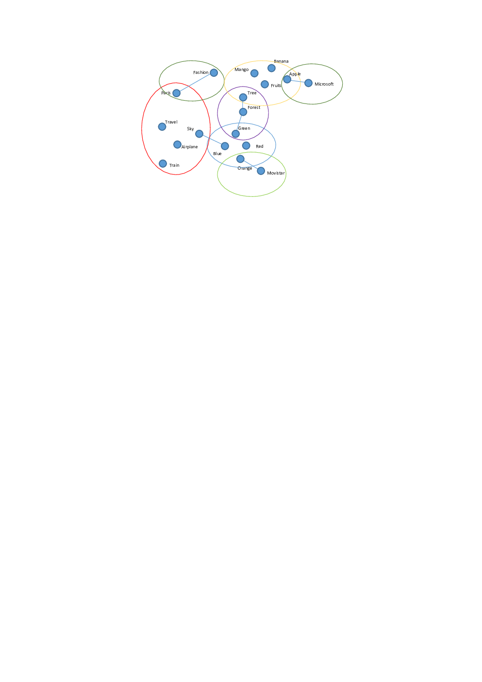

A word embedding : is a parameterized function mapping words to high-dimensional vectors (Chen2017). Typically, the function is a lookup table, parameterized by a matrix, , with one row for each word: . is initialized with a random vector for each word. During the training, it learns meaningful vectors in order to perform some task. The resulting embedding vectors can be interpreted as semantic features, and can be used to understand similarities or differences between words. The distance between vectors describes their semantic similarity. Using the numeric/semantic vectors, it is possible to gain additional insights, as shown in figure 5 for an NLP example. We observe that words with a similar semantic meaning are close to each other in the 2-dimensional projection of the embedding space. In this paper, we utilize the advantage that an embedding layer turns categorical variables into vectors. We use the concept of word embedding to encode the calendar features (month, weekday, hour) into a neural network. The resulting embedding vectors are used for two purposes:
- 1.
As features in the neural network representing calendar information
- 2.
To graphically understand how electricity prices behave depending on time variables and derive economical insights
Proposed neural network
In this paper we propose a dense neural network with an embedding layer to encode the calendar information. Figure 6 illustrates the network. The input features are calendar data and, in some applications, infeed forecasts for renewables. The actual neural network consists of two hidden layers with Relu (Rectified Linear Unit) activation and an output layer with linear activation (as this is a regression task). In section 4 we will describe the models and parameters in more detail.
Embedding layer for calendar features
The embedding layer is used to encode the calendar information. Embeddings are an alternative to one-hot-encoding of categorical features. As for every layer in a neural network including the embedding layer, the number of neurons has to be chosen carefully (the number of dimensions is a hyperparameter you can tweak geron2019hands on embeddings). Scientific literature does not provide explicit guidelines and, to the best of our knowledge, embeddings have not been used in EPF so far. However, there are some studies on the dimensionality of word embeddings (Yin2018; Gu2020; Wendlandt2018). The authors point out the importance of a correct choice of the dimensionality of the embedding, as a high dimension can lead to overfitting and a very low dimension can not capture all the meaning of the categorical variable. Most of these studies agree that the dimension must be selected empirically as it depends on the data. We optimized the dimension between 15 % and 35 % in 5% intervals and found that 25 % gives the best overall results, even though the differences were rather small.
We consider the following embedding variables:
- •
Hour: The categorical variable takes values in , so in a one-hot-encoding it has dimension 24. For its embedding dimension we chose six.
- •
Weekday: The categorical variable takes values in , where depends on the representation of holidays outlined below. Its embedding dimension is two. We consider three approaches to deal with holidays:
- –
Approach 1: weekday considering each weekday (Sunday, Monday, … Saturday) separately and adding a category for holidays.
- –
Approach 2: weekday considering seven weekdays and three types of holidays: Partial holiday, public holiday and bridge day 33 3 Bridge, partial, and public holiday describe days with influence through public holidays. Public is the actual public holiday, partial is a public holiday in only parts of Germany and bridge describes days between a public holiday and weekends..
- –
Approach 3: This approach uses two embedding variables, i.e. treating holiday and weekday separately. This is motivated by the fact, that every holiday also has an associated weekday (i.e. Easter Sunday is a holiday, but also a Sunday): weekday and type_holiday .
A list of holidays used is in appendix . In this paper we present the results for Approach 2, as it gave the mean absolute deviation. The interested reader can get detailed results for Approaches 1 and 3 by contacting the authors.
- –
- •
Month: The categorical variable takes values in and its embedding dimension is three.
- •
Year: The categorical variable takes values in and its embedding dimension is three.
- •
Cross-feature month-hour: Due to differences in daylight hours, there is a relationship in electricity demand between month and hour-of-the-day. The categorical variable takes values in and its embedding dimension is ten.
- •
Cross-feature weekday-hour: Due to differences in human behaviour (e.g. people get up later on the weekend) there is a relationship in electricity demand between weekday and hour. The categorical variable takes values in and its embedding dimension is fifteen.
4 Empirical performance on the German electricity market
In this section we carry out an experimental study on the German electricity market. We distinguish the two applications as outlined in detail in section 2. In both applications we conduct a statistical analysis to show the significance of the results.
- Short-term forecasting:
-
For the short-term forecasting we use a DNN with an embedding layer to encode the calendar information and six different benchmark models. Four of them are neural network models, one is a time series approach and one is a naive method. In addition to calendar information we also use forecasts on renewable infeed (wind and photovoltaic) as features (see below for details).
We follow a training framework with daily recalibration, so we retrain the model every day with historical data available. As we forecast the day-ahead market, which is traded at 12 o’clock for the next day, we can rely our model on prices up to the current day (which was traded the day-before) and forecasts on renewable infeed for the next day. In our experimental study we use a history of five years to train the model. In other words, using a five-year history of the data available up to the time the prediction model is run, the model predicts the prices for each of the next 24 hours.
- Long-term profile forecasting:
-
For the long-term forecasting we use a DNN with an embedding layer and, as a benchmark, popular methods from the literature (dummy variables and sinusoidal). We forecast four years ahead.
Data
For our study we use data from the German44 4 Note that the German spot market had been a larger market including Austria (EPEX DE/AT) until October 1st 2018. Day-Ahead electricity market (EPEX DE) from 2010 through 201955 5 Due to missing data from EEX Transparency, we excluded 11/01/2010 and 10/02/2010 from our analysis., as traded on EPEX Spot66 6 https://www.epexspot.com/en/market-data. We also use data on the expected generation from renewables in Germany, which we collect from the EEX transparency platform77 7 https://www.eex-transparency.com/power/de/production/usage/. We compiled our data sets from FTP-files which we licensed from the German Energy Exchange EEX88 8 https://www.eex.com/de/marktdaten/strom, but the data can be viewed without a license on the corresponding websites. More details on the data are in table 1. We use an Ex-Ante timestamp (i.e. hour 1 describes the price or renewable infeed for the time between 1:00 AM and 2:00 AM).
It is a known fact that neural networks work much better when variables are normalized. That is why in our experimental study the renewable variables are scaled using a technique known as standard scaler:
| (3) |
The values and are computed over the training set only. The prices were not normalized in our models because they are the output feature (makes no difference in training), except for the LSTM models, which use prices also as an input feature.
| EPEX DE(/AT) | Expected production | ||
|---|---|---|---|
| Photovoltaic | Wind | ||
| Features | date, price | date, expected volume | date, expected volume |
| Start date | 1/1/2010 | 1/1/2010 | 1/1/2010 |
| Final date | 31/12/2019 | 31/12/2019 | 31/12/2019 |
The evaluation metric used in this study is the mean absolute error (MAE):
| (4) |
where is the number of hours, is the realized price on the exchange and is the predicted price.
Short-term forecasting
This section summarizes the results of the day-ahead forecasting of hourly prices. We compare our proposed neural networks using embeddings and benchmarks from the literature.
Setup
For the experimental study we design different configurations for DNN and LSTM models, see table 2 and 3.
In general there are alternative approaches to include calendar information in neural networks. We compare the embedding approach to two alternatives:
- •
Using ordinal variables:
- –
weekday: numeric variable
- –
month: numeric variable
- –
hour: numeric variable
- –
- •
| (5) |
| (6) |
To select the configurations for the DNN we follow recommendations from Kapoor2019 and use the formula in equ. (7) (as also referenced in a blog-post (Hyperparater2018) on the towardsdatascience.com-website, a platform very popular among practitioners):
| (7) |
is the number of input neurons, the number of output neurons, the number of samples in the training data, and represents a scaling factor that is usually between 2 and 10. We calculate and compare the following models to forecast the 24 hourly prices of the next day.
We compare the following model architectures. For most of them we do calculations with two sets of features, namely only calendar information as well as calendar information and renewables (forecasts on the infeed of wind and photovoltaic/solar energy).
- Naive
-
A naive model using past prices. The output of the naive method for hour of date is the price at hour of the last observed day of the same type (e.g. working day, Saturday).
- LEAR
-
LASSO Estimated Auto-Regressive model is one of two benchmark models presented in LAGO2021. The model is based on a parameter-rich ARX (Auto-Regressive with exogenous features) structure which is estimated by LASSO (least-absolute-shrinkage and selection operator). They show that long calibration windows (three and four years) lead to the best results. For our LEAR model we chose five years as calibration window, as we used the same time frame for the recalibration of our DNN models.
- LSTM
-
Neural-network with LSTM-architecture and configuration as in table 3.
- DNN-Lago
-
Dense neural network, which is the second benchmark model presented in LAGO2021. This model is based on a multivariate framework. The input features and hyperparameters of every model configuration are calculated in a separate pre-processing using Bayesian optimization. We use the first five years of our dataset for the hyperparamter optimization. The resulting configurations are shown as configurations c4 and c5 in table 2.
- DNN-ordinal
-
Dense neural network with three different configurations c1, c2 and c3 as shown in table 2. This model is also evaluated without calendar information using only renewables as features.
- DNN-sin-cos
-
Dense neural network with three different configurations c1, c2 and c3 as shown in table 2. Calendar information is encoded as a circle function as in schnuerchWagner2020.
- DNN-embedding
-
Our approach as presented in the previous section. We use three different configurations c1, c2 and c3 as shown in table 2.
The models are trained on the last five years preceding the day we forecast and are retrained daily. Training the LSTM models is computationally extensive and could take more than one day in practice. For this reason we use a simple configuration for our experimental study. All DNN configurations are summarized in table 2. We use MSE as loss function. Note that we do show only the most important hyperparameters for the sake of clarity.
| Parameters | c1 | c2 | c3 | c4 | c5 |
|---|---|---|---|---|---|
| Hidden layers | 1 | 2 | 2 | 2 | 2 |
| Neurons per layer | 2085 | 128/128 | 2285/1024 | 484/381 | 234/203 |
| Activation layers | Relu | Relu | Relu | Sigmoid | Relu |
| Epochs | 10 | 10 | 10 | auto | auto |
| Optimizer | RMSprop | RMSprop | RMSprop | Adam | Adam |
| Parameters | |
|---|---|
| Hidden layers | 3 |
| Neurons per layer | 10/10/24 |
| Type of layer | LSTM/LSTM/dense |
| Activation layers | Relu |
| Epochs | 10 |
| Optimizer | Adam |
Results
We predict the next 24 hours using the past five years of data. We repeat these experiments for every day starting on the 1st of January 2015. Note that, therefore, all results are out-of-sample and provide a valid benchmark for use in practice. In the following, we present the mean hourly absolute error per year, for every different configuration and training sample. Any interested reader can get detailed results (every hour) by contacting the authors. Table 4 shows the results.
| Method | Features | Config. | 2015 | 2016 | 2017 | 2018 | 2019 | |
|---|---|---|---|---|---|---|---|---|
| LSTM | renewables | - | 7.12 | 6.52 | 7.94 | 9.38 | 8.77 | |
| Naive | - | - | 7.34 | 6.19 | 9.89 | 10.43 | 9.77 | |
| LEAR | renewables | - | 4.22 | 4.26 | 4.70 | 5.92 | 4.84 | |
| DNN-Lago | renewables | c4 | 3.68 | 3.70 | 5.32 | 5.01 | 4.52 | |
| c5 | 3.76 | 3.52 | 4.56 | 4.77 | 4.53 | |||
| DNN-ordinal | renewables | c1 | 8.30 | 6.98 | 9.76 | 9.77 | 9.49 | |
| c2 | 8.23 | 6.69 | 9.66 | 9.52 | 9.11 | |||
| c3 | 8.51 | 6.88 | 9.56 | 9.83 | 8.72 | |||
| calendar | c1 | 7.76 | 6.76 | 9.87 | 10.06 | 9.10 | ||
| c2 | 7.78 | 6.71 | 9.77 | 10.15 | 9.11 | |||
| c3 | 7.21 | 6.47 | 9.38 | 9.87 | 8.65 | |||
| + renewables | c1 | 5.44 | 4.98 | 7.05 | 6.73 | 6.97 | ||
| c2 | 5.57 | 4.92 | 7.03 | 6.83 | 7.14 | |||
| c3 | 5.16 | 4.66 | 6.52 | 6.63 | 6.15 | |||
| DNN-sin-cos | calendar | c1 | 7.06 | 5.93 | 8.93 | 10.05 | 8.18 | |
| c2 | 6.71 | 5.67 | 8.75 | 9.33 | 8.01 | |||
| c3 | 6.26 | 5.47 | 8.48 | 8.70 | 7.59 | |||
| + renewables | c1 | 4.29 | 3.93 | 5.58 | 5.89 | 5.83 | ||
| c2 | 4.13 | 3.72 | 5.43 | 5.51 | 5.39 | |||
| c3 | 3.88 | 3.49 | 4.85 | 4.90 | 4.77 | |||
| DNN-embedding | calendar | c1 | 5.92 | 5.06 | 8.11 | 8.44 | 8.41 | |
| c2 | 6.04 | 5.25 | 8.16 | 8.38 | 7.37 | |||
| c3 | 5.86 | 5.00 | 7.87 | 8.19 | 7.24 | |||
| + renewables | c1 | 3.78 | 3.42 | 5.12 | 4.93 | 5.00 | ||
| c2 | 3.82 | 3.38 | 5.09 | 4.98 | 4.78 | |||
| c3 | 3.50 | 3.21 | 4.69 | 4.65 | 4.46 |
Our proposed approach based on embeddings performs well compared to the benchmarks. The DNN-embeddings + renewables approach has an overall MAE of 4.10 EUR/MWh for its best configuration (DNN-emb-renew-c3). Other competitive approaches include DNN-Lago (4.23) and DNN-sin-cos (4.38). Figure shows an example of hourly prediction for September of 2016 using renewables and embeddings for calendar information. It can be observed that our model is able to nicely capture the seasonal structure.
We can conclude that our proposed method is very competitive with the existing state-of-the-art machine-learning based forecast of electricity prices. However, we think that it provides those good results with a fairly simple model architecture. In order to statistically support our findings we conduct an extensive analysis using non-parametric tests in the following.