The gravitational wave background signal from tidal disruption events20202020The gravitational wave background signal from tidal disruption events–References

Let us consider a star of mass $M_{*}$ and radius $R_{*}$, on a parabolic orbit around a non-spinning black hole of mass $M_{\rm h}$. The TDE takes place when the tidal forces due to the BH overcome the stellar self-gravity. For the purpose of the present paper, it is sufficient to use the so-called impulse approximation, which means that the star interacts with the hole only at the pericenter $r_{\rm p}$, where it gets disrupted. Because of the varying quadrupole moment of the BH-star system, we expect a GW burst at pericenter (Kobayashi et al. 2004). A simple estimate of the (maximum) GW strain emitted by the source is (see, e.g., Thorne 1998)

where ${\color[rgb]{0,0,0}d}$ is the distance of the source from Earth and $E_{\rm kin}$ is the kinetic energy of the star, since due to the high mass ratio between the BH and the star we can consider the BH at rest in the centre of mass frame (see appendix A of Toscani et al. 2019 for a more detailed discussion on this assumption). Assuming the star to be a point-like particle in Keplerian motion, we write $E_{\rm kin}$ as

Thus, the GW strain becomes

with an associated frequency

where we have introduced the Schwarzschild radius $r_{\rm s}$ of the BH, the Schwarzschild radius $r_{\rm s*}$ of the star, and the maximum pericenter distance for tidal disruption (a.k.a tidal radius)

In fact, $r_{\rm t}$ should have also a numerical factor of a few, due to the internal structure of the star, relativistic effects in the process of disruption and other physical details of the system. We take this factor to be 1 for simplicity. The penetration factor $\beta$ is defined as

This factor varies between a minimum value $\beta_{\rm min}=1$ (i.e. $r_{\rm p}=r_{\rm t}$), and a maximum value $\beta_{\rm max}=r_{\rm t}/r_{\rm s}$, when the pericenter is equal to the BH Schwarzschild radius. Within this radius the star is directly swallowed rather than disrupted by the BH. For $\beta=1$ and a Sun-like star disrupted by a $10^{6}\,\text{M}_{☉}$ static BH at $\approx 16\,\text{Mpc}$ from us, equations (3)-(4) give $h\approx 10^{-22}$ and $f\approx 10^{-4}\,\text{Hz}$ (cf. Kobayashi et al. 2004).

Before developing the calculations in a more formal way, we can give an estimate of the GW background from MS stars and WDs in the following way. We approximate the FT of the strain as $h/f$ (we will justify why it is possible to do this in section 3) and we write

where $N^{\rm tde}$ is the number of tidal disruption events, $\dot{N}^{\rm tde}_{\rm gal}$ is the rate of TDEs per galaxy and $N^{\rm gal}$ is the number of galaxies. Thus, we can write equation (31) as

If we consider a Sun-like star disrupted by a $10^{6}\,\text{M}_{☉}$ BH, we have that the frequency is $\approx 10^{-4}\,\text{Hz}$ (cf. section 2.1) and the TDE rate is $\dot{N}^{\rm tde}_{\rm gal}\approx 10^{-4}\text{yr}^{-1}\,\text{gal}^{-1}$ (see, e.g., Stone & Metzger 2016). If we consider about 0.01 galaxies per unit of cubic Megaparsec (see, e.g, Montero-Dorta & Prada 2009), we can estimate that up to $z\sim 1$ (i.e. $4\times 10^{3}\,\text{Mpc}$) there are $0.01\,\text{gal}/\text{Mpc}^{3}\times(4\times 10^{3}\,\text{Mpc})^{3}\approx 10^{8}\,\text{galaxies}$. Inserting all this information in equation (33), we get

So we expect the GW background from TDEs of MS stars to be around the same order of magnitude of the the strain from the single event. Moreover, if we compare the background from MS stars and the one from WDs we obtain

and considering a MS star as in the previous example, and a WD disrupted by a $10^{5}\,\text{M}_{☉}$ BH with an estimated rate of $\dot{N}^{\rm WD}_{\rm gal}\approx{\color[rgb]{0,0,0}10^{-4}}\,\text{/y/gal}$ (see, e.g., Stone & Metzger 2016), we have

So the background of Sun-like stars disrupted by a $10^{6}\,\text{M}_{☉}$ BH is around the same order of magnitude as the background of WDs disrupted by a ${\color[rgb]{0,0,0}10^{5}}\,\text{M}_{☉}$ BH and, since both the signals are not very strong, we do not expect them to be detected (at least for LISA and TianQin). However, if we assume that these WDs are disrupted not in galactic nuclei but by IMBHs residing in globular clusters, with a disruption rate around $\dot{N}^{\rm WD}_{\rm gc}\approx{\color[rgb]{0,0,0}10^{-3}}/\text{y}/\text{gc}$ (see, e.g., Baumgardt et al. 2004a), we get

Thus, if we take into account WDs disrupted by IMBHs in globular clusters, the estimated number of GCs per galaxy becomes a key factor in the derivation of this background. Now that we have explored the expected magnitude of the background, we move to a full description of the physical scenario at hand.

We need to find the proper expression for $d\#/dtdz$. Since we assume a fixed stellar mass, the other possible variables that this quantity can depend on, apart from $z$ and $t$, are the mass of the IMBH in the GC, $M_{\rm h}$, and the number of GCs per galaxy, $N_{\rm gal}^{\rm gc}$. We assume that the mass distribution of IMBHs is a $\delta$ function at a fixed value of $M_{\rm h}$, that we take as a free parameter in the range $10^{3}\text{M}_{☉}\leq M_{\rm h}\leq 10^{5}\text{M}_{☉}$. So, the only variable left is $N_{\rm gal}^{\rm gc}$. It is reasonable to assume that there is a scale relation between this quantity and the luminosity of the galaxy that hosts the GCs. Since this luminosity can be more conveniently expressed in terms of the mass of the SMBH in the nucleus of the galaxy, $M_{\bullet}$ (see, e.g., Faber & Jackson 1976 and Ferrarese & Merritt 2000), we can write

In particular, equation (38) can be expressed as

where $\dot{N}_{\rm gc}^{\rm tde}$ is the rate of TDEs of WDs per globular cluster, $N_{\rm gal}^{\rm gc}$ is the number of globular clusters per galaxy, ${dn}/{dM_{\rm\bullet}}$ is the number density of galaxies per unit SMBH mass and ${dV_{\rm c}}/{dz}$ is the comoving volume per redshift slice $dz$. In the following paragraphs we explicit each term of equation (39).

For MS stars, the number of sources per unit of time per unit of redshift will depend on the mass of the SMBH involved in the disruption, $M_{\bullet}$, so we can write

For the term $\dot{N}^{\rm tde}_{\rm gal}$, we need to consider that this rate will depend on both the stellar mass and the distance between the star and the black hole (see section 3.1.1 for the considerations about full and empty loss cone). If we assume

where $\phi(M_{*})$ is the Salpeter function (Salpeter 1955) normalized in the interval $[1,+\infty)$

we can write

In the calculations we take $M_{*}=100\,\text{M}_{☉}$ and $\beta=r_{\rm t}/r_{\rm s}$ as upper limits for $M_{*}$ and $\beta$ rispectively. For the rate, we take the one calculated by Stone & Metzger 2016

We need to specialize equation (25) for TDEs, which means that we have to find the expression for $\tilde{h}(f)$. In paragraph 2.1 we have explained that it is suitable to approximate this GW signal from TDEs with a burst. Thus, we are in practice considering the strain like a constant function over the interval [-$\tau$/2,$\tau$/2] (where $\tau$ is the duration of the signal), and zero outside. For these reasons, we can write the FT of the signal as

so that equation (22) can be expressed as

where we have considered that the strain does not depend on the orientation of the source for our problem. Thus, equation (67) becomes

(in the last step, we consider $\beta\propto f^{2/3}$, cf. section 2).

Considering all the steps illustrated in the previous sections, the final formula for the background is

where $\mathcal{A}_{\rm WD}$ is a model dependent constant given by

with

In the calculation, we have taken a GC core density $n_{\rm c}\approx 10^{5}\,\text{pc}^{-3}$ and core radius $r_{\rm c}\approx 0.5\,\text{pc}$. The mass dimensionless variable $\mathcal{M}=M_{\bullet}/10^{8}\text{M}_{☉}$ ranges in the interval $10^{-2}\leq\mathcal{M}\leq 1$, spanning the mass range $10^{6}\text{M}_{☉}-10^{8}\text{M}_{☉}$. The term in square brackets results from the integral over the parameter $\beta$, so we have this term only when considering the full loss cone scenario. We report in Tables 1-2 the typical values of $\mathcal{A}_{\rm WD}$ for different choices of the parameters, in the empty and full loss cone, respectively.
Let us estimate the frequency range we expect the signal to cover. The observed frequency is related to the rest frame frequency by $f=f_{\rm r}/(1+z)$. So, when the redshift is zero, the observed frequency coincides with the frequency of the source, meanwhile for higher redshifts $f$ decreases, approaching 0 for $z\rightarrow\infty$.

However, although in the above integral we consider $0\leq z<\infty$, from a physical point of view we expect most of the signal to be collected from within a finite redshift $z_{\rm max}$ that we derive by inspecting $\mathcal{I}(z)$ in equation (71). This function is plotted in Figure 1 for two extreme values of the parameter $\lambda$, i.e. $\lambda=1$ and $\lambda=2.2$, setting $f_{\rm r}=0.07\,\text{Hz}$.

The function vanishes for $z\geq 3$, thus the lowest frequency at which we observe the signal is $f\approx 0.07/4=0.02~\text{Hz}$. We therefore expect the frequency interval of the background signal in the empty loss cone regime to be $[0.02~\text{Hz},0.07~\text{Hz}]$. In the full loss cone scenario $\beta$ is not fixed to 1, so in order to derive the observed frequency interval, we need to consider both $z_{\rm max}$ and the maximum value of $\beta$ (see paragraph 2). The result is the following

Note that for $M_{\rm h}=10^{5}\text{M}_{☉}$, the range of frequency is almost the same as for the empty loss cone since the allowed $\beta$ range is small and around $\beta\approx 1$. Indeed, $M_{\rm h}=10^{5}\text{M}_{☉}$ is a limit situation for the full loss cone scenario, but we have decided to include also this case for completeness. It follows that the natural frequency range for this physical system goes from the decihertz to a few hertz. For this reason, we compare our results with the sensitivity curves of the following (future) space interferometers: LISA (Amaro-Seoane et al. 2017), TianQin (Luo et al. 2016), ALIA (Bender et al. 2013 and Baker et al. 2019), DECIGO (Sato et al. 2017) and the BBO (Harry et al. 2006), that are all shown in Figure 2.
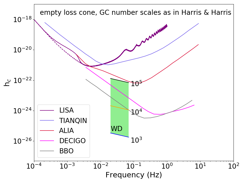
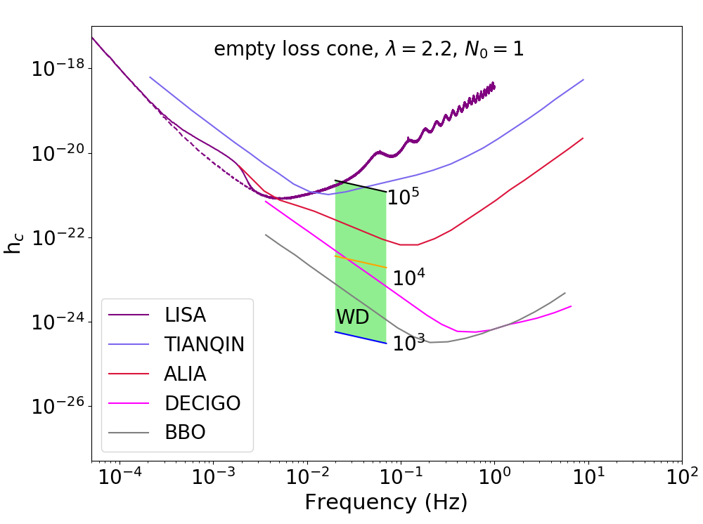
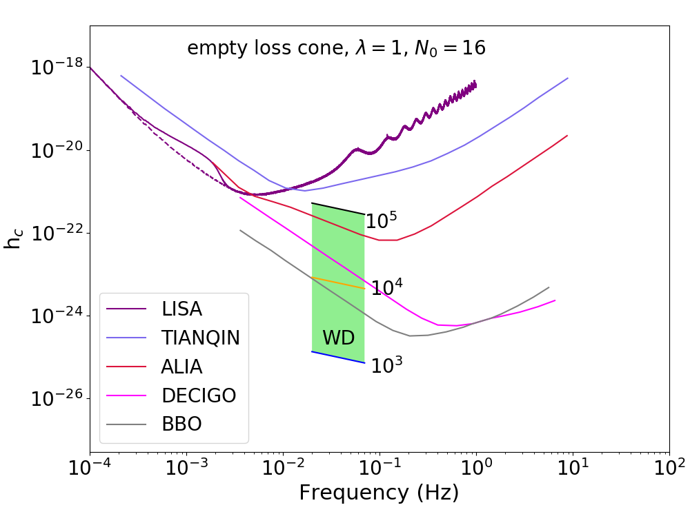
Our results are illustrated in Figures 3-4-5. We explore how the background varies if we change the parameters $M_{\rm h},\lambda\,\,\text{and}\,\,N_{0}$. In Figure 3 we illustrate the results for the (pessimistic) case $\lambda=1$ and $N_{0}=1$, that is the scenario where we assume the same linear relation between the number of globular clusters in a galaxy and the mass of the super massive black hole in its core as in Burkert & Tremaine 2010 and in Harris & Harris 2011. Then, we show the results also for the more optimistic case where $\lambda$ and $N_{0}$ satisfying the conditions for the MW, in particular $\lambda=2.2$ and $N_{0}=1$ in Figure 4, while $\lambda=1$ and $N_{0}=16$ in Figure 5, since these are the two cases where, for a fixed $M_{\bullet}$, we have the highest number of GCs. In each figure, in the left plot we show the empty loss cone scenario, while the full loss cone is illustrated in the right plot. The blue, orange and black lines represent the GW background if we assume that all the IMBHs have same mass equal to $10^{3},10^{4},10^{5}\,\text{M}_{☉}$ respectively. The green area represents the cases with a IMBH mass in between these values. So the actual background of these events will be inside this green area. In all the cases illustrated, the GW background may be detected by DECIGO and it is always above BBO sensitivity curve. It may also be visible to ALIA for the cases $\lambda=2.2,\,N_{0}=1$ and $\lambda=1,\,N_{0}=16$, if we consider high BH masses. Moreover, in the most optimistic scenario ($\lambda=2.2,\,N_{0}=1$), the signal even grazes TianQin sensitivity curve.
These results suggest that the TDE background signal from WDs could be indeed detected by both DECIGO and BBO, maybe even by ALIA and surely by any interferometers that will work in the decihertz band with a higher sensitivity than the planned ones.

In the case of MS stars, the final formula of the background is

where $\mathcal{A}_{\rm MS}$ is a constant model dependent

with

References

- Amaro-Seoane & Spurzem (2001) Amaro-Seoane P., Spurzem R., 2001, MNRAS, 327, 995
- Amaro-Seoane et al. (2017) Amaro-Seoane P., et al., 2017, arXiv e-prints,
- Anninos et al. (2018) Anninos P., Fragile P. C., Olivier S. S., Hoffman R., Mishra B., Camarda K., 2018, ApJ, 865, 3
- Bahcall & Wolf (1977) Bahcall J., Wolf R., 1977, The Astrophysical Journal, 216, 883
- Baker et al. (2019) Baker J., et al., 2019, preprint
- Baumgardt et al. (2004a) Baumgardt H., Makino J., Ebisuzaki T., 2004a, ApJ, 613, 1133
- Baumgardt et al. (2004b) Baumgardt H., Makino J., Ebisuzaki T., 2004b, ApJ, 613, 1143
- Bender et al. (2013) Bender P. L., Begelman M. C., Gair J. R., 2013, Classical and Quantum Gravity, 30, 165017
- Blaes & Glatzel (1986) Blaes O. M., Glatzel W., 1986, MNRAS, 220, 253
- Bloom et al. (2011) Bloom J. S., et al., 2011, Science, 333, 203
- Bonnerot et al. (2016) Bonnerot C., Rossi E. M., Lodato G., Price D. J., 2016, MNRAS, 455, 2253
- Burkert & Tremaine (2010) Burkert A., Tremaine S., 2010, ApJ, 720, 516
- Einstein (1918) Einstein A., 1918, Sitzungsberichte der Königlich Preußischen Akademie der Wissenschaften (Berlin), Seite 154-167.
- Faber & Jackson (1976) Faber S. M., Jackson R. E., 1976, ApJ, 204, 668
- Ferrarese & Merritt (2000) Ferrarese L., Merritt D., 2000, The Astrophysical Journal, 539, L9
- Frank & Rees (1976) Frank J., Rees M. J., 1976, Monthly Notices of the Royal Astronomical Society, 176, 633
- Gabasch et al. (2006) Gabasch A., et al., 2006, Astronomy and Astrophysics s, 448, 101
- Gezari et al. (2017) Gezari S., Cenko S. B., Arcavi I., 2017, ApJ, 851, L47
- Guillochon & Ramirez-Ruiz (2013) Guillochon J., Ramirez-Ruiz E., 2013, ApJ, 767, 25
- Guillochon et al. (2009) Guillochon J., Ramirez-Ruiz E., Rosswog S., Kasen D., 2009, ApJ, 705, 844
- Haas et al. (2012) Haas R., Shcherbakov R. V., Bode T., Laguna P., 2012, ApJ, 749, 117
- Harris & Harris (2011) Harris G. L. H., Harris W. E., 2011, MNRAS, 410, 2347
- Harry et al. (2006) Harry G. M., Fritschel P., Shaddock D. A., Folkner W., Phinney E. S., 2006, Classical and Quantum Gravity, 23, 4887
- Hayasaki et al. (2013) Hayasaki K., Stone N., Loeb A., 2013, Monthly Notices of the Royal Astronomical Society, 434, 909
- Hayasaki et al. (2016) Hayasaki K., Stone N., Loeb A., 2016, MNRAS, 461, 3760
- Hogg (1999) Hogg D. W., 1999, ArXiv Astrophysics e-prints,
- Kiuchi et al. (2011) Kiuchi K., Shibata M., Montero P. J., Font J. A., 2011, Phys. Rev. Lett., 106, 251102
- Kobayashi et al. (2004) Kobayashi S., Laguna P., Phinney E. S., Meszaros P., 2004, ApJ, 615, 855
- Komossa (2015) Komossa S., 2015, Journal of High Energy Astrophysics, 7, 148
- Komossa et al. (2008) Komossa S., et al., 2008, ApJ, 678, L13
- Lin & Tremaine (1980) Lin D., Tremaine S., 1980, The Astrophysical Journal, 242, 789
- Lin et al. (2018) Lin D., et al., 2018, Nature Astronomy, 2, 656
- Lin et al. (2020) Lin D., et al., 2020, ApJ, 892, L25
- Lodato & Rossi (2011) Lodato G., Rossi E. M., 2011, MNRAS, 410, 359
- Lodato et al. (2009) Lodato G., King A. R., Pringle J. E., 2009, MNRAS, 392, 332
- Luo et al. (2016) Luo J., et al., 2016, Classical and Quantum Gravity, 33, 035010
- Maggiore (2007) Maggiore M., 2007, Gravitational Waves. Volume 1: Theory and Experiments. Oxford University Press
- McConnell & Ma (2013) McConnell N. J., Ma C.-P., 2013, ApJ, 764, 184
- Montero-Dorta & Prada (2009) Montero-Dorta A. D., Prada F., 2009, MNRAS, 399, 1106
- Moore et al. (2015) Moore C. J., Cole R. H., Berry C. P. L., 2015, Classical and Quantum Gravity, 32, 015014
- Papaloizou & Pringle (1984) Papaloizou J. C. B., Pringle J. E., 1984, MNRAS, 208, 721
- Peng et al. (2019) Peng Z.-K., Yang Y.-S., Shen R.-F., Wang L.-J., Zou J.-H., Zhang B.-B., 2019, arXiv e-prints
- Phinney (1989) Phinney E. S., 1989, in Morris M., ed., IAU Symposium Vol. 136, The Center of the Galaxy. p. 543
- Phinney (2001) Phinney E. S., 2001, arXiv Astrophysics e-prints,
- Rees (1988) Rees M. J., 1988, Nature, 333, 523
- Rosswog (2009) Rosswog S., 2009, New Astron. Rev., 53, 78
- Salpeter (1955) Salpeter E. E., 1955, Astrophysical Journal, 121, 161
- Sato et al. (2017) Sato S., et al., 2017, Journal of Physics: Conference Series, 840, 012010
- Schechter (1975) Schechter P., 1975, PhD thesis, California Institute of Technology, Pasadena, CA USA
- Sesana et al. (2008) Sesana A., Vecchio A., Colacino C. N., 2008, MNRAS, 390, 192
- Shapiro & Teukolsky (1983) Shapiro S. L., Teukolsky S. A., 1983, Black holes, white dwarfs, and neutron stars: The physics of compact objects
- Shiokawa et al. (2015) Shiokawa H., Krolik J. H., Cheng R. M., Piran T., Noble S. C., 2015, ApJ, 804, 85
- Stone & Metzger (2016) Stone N. C., Metzger B. D., 2016, Monthly Notices of the Royal Astronomical Society, 455, 859
- Stone et al. (2013) Stone N., Sari R., Loeb A., 2013, Monthly Notices of the Royal Astronomical Society, 435, 1809
- Thorne (1998) Thorne K. S., 1998, Probing Black Holes and Relativistic Stars with Gravitational Waves. University of Chicago Press (arXiv:gr-qc/9706079)
- Toscani et al. (2019) Toscani M., Lodato G., Nealon R., 2019, MNRAS, 489, 699
- Young (1977) Young P., 1977, The Astrophysical Journal, 215, 36
- van Putten (2001) van Putten M. H., 2001, Phys. Rev. Lett., 87, 091101
- van Putten et al. (2019) van Putten M. H. P. M., Levinson A., Frontera F., Guidorzi C., Amati L., Della Valle M., 2019, European Physical Journal Plus, 134, 537