Minimum Overhead Beamforming and Resource Allocation in D2D Edge Networks
Abstract
Device-to-device (D2D) communications is expected to be a critical enabler of distributed computing in edge networks at scale. A key challenge in providing this capability is the requirement for judicious management of the heterogeneous communication and computation resources that exist at the edge to meet processing needs. In this paper, we develop an optimization methodology that considers the network topology jointly with device and network resource allocation to minimize total D2D overhead, which we quantify in terms of time and energy required for task processing. Variables in our model include task assignment, CPU allocation, subchannel selection, and beamforming design for multiple-input multiple-output (MIMO) wireless devices. We propose two methods to solve the resulting non-convex mixed integer program: semi-exhaustive search optimization, which represents a “best-effort” at obtaining the optimal solution, and efficient alternate optimization, which is more computationally efficient. As a component of these two methods, we develop a novel coordinated beamforming algorithm which we show obtains the optimal beamformer for a common receiver characteristic. Through numerical experiments, we find that our methodology yields substantial improvements in network overhead compared with local computation and partially optimized methods, which validates our joint optimization approach. Further, we find that the efficient alternate optimization scales well with the number of nodes, and thus can be a practical solution for D2D computing in large networks.
Index Terms:
Wireless edge networks, device-to-device (D2D) communications, multiple-input-multiple-output (MIMO), beamforming, network optimization.I Introduction
The number of wireless devices is now over billion, and with the advent of new 5G-and-beyond technologies, this is expected to grow to billion by 2022 [2]. Many of these devices will be data-processing-capable nodes in the hands of users that facilitate rapidly growing data-intensive applications running at the network edge, e.g., social networking, video streaming, and distributed data analytics. Given the bursty nature of user demands, when certain devices are occupied with processing for computationally-intensive applications, e.g., face recognition, 3D modeling/gaming, and augmented/virtual reality (AR/VR), it may be desirable for them to offload their data to devices with underutilized resources [3, 4, 5]. Traditionally, cloud computing architectures, such as Amazon Web Services and Microsoft Azure, have been adopted for such data intensive applications, but the exponential rise in data generation at the edge is making centralized architectures infeasible for providing latency-sensitive quality of service at scale [2].
As a current trend in wireless networks is reducing cell sizes [6], many 5G networks will be dense with small cell coverage areas and networks composed of several smaller subsets [7]. Networks of small subnets combined with improved computational and storage capabilities of edge devices are enabling mobile edge computing (MEC) architectures. At a high level, MEC leverages radio access networks (RANs) to increase the amount of computing power located close to the end user, which enables the end user to offload computations (e.g., using a central processing entity) as shown in Fig. 1(1(a)) [8, 9, 10, 11, 12, 13, 14, 15, 16, 17]. In an MEC architecture, the edge servers have high-performance computing units which can process large amounts of computationally intensive tasks efficiently. This concept has been extended to “helper” edge server architectures as well, where devices with idle computation resources become (small) edge servers [18, 19, 20, 21, 22, 23].


The current trend in distributed computing, though, is a migration to architectures that are more decentralized than MEC. This is due to the fact that all edge nodes can take part in data offloading at different times because of the advances in 5G communication technologies in conjunction with improved computational capabilities of individual devices. For this reason, device-to-device (D2D) network architectures (in Fig. 1(1(b))) that were previously studied in 4G LTE standards now hold the promise of providing distributed computing at scale [24].
Unlike the MEC system in Fig. 1(1(a)), distributed computing in the D2D network of Fig. 1(1(b)) will have more complicated topology management needs that must be considered together with the management of device resources. From a computation perspective, the edge nodes that receive offloaded tasks must have a suitable strategy for allocating its central processing unit (CPU) and/or storage resources to the tasks. From a communication perspective, wireless transmissions between edge nodes will inevitably incur inter-channel interference due to concurrent data offloading. In contemporary wireless networks, devices are often equipped with multiple antennas to support multiple input multiple output (MIMO) communications, and the ability to communicate over different subchannels. Theoretically, having both multiple transmit and multiple receive antennas (i.e., a MIMO channel) provides an additional spatial dimension for communication and yields a degree-of-freedom gain [25], which can be leveraged to mitigate such inter-channel interference. This motivates interference management techniques that consider the joint effects of subchannel allocations, transmission powers, MIMO beamforming, and other device transmit resources.
The focus of this paper is on addressing these challenges. Specifically, we develop methodologies that jointly optimize computation and communication resources together with topology configuration in D2D wireless edge computing systems. These methodologies will aim to minimize the overhead incurred from communication and computation, measured in terms of time delay/latency and energy consumption incurred from processing tasks in the D2D network.
I-A Related Work and Differentiation
We discuss related works on task offloading, resource management, and edge computing. We divide our analysis into two main categories: MEC and D2D.
I-A1 MEC systems
Researchers have developed methods for resource management and offloading decision-making to maximize MEC system performance. Offloading decisions were thoroughly studied in [8], where management of device resources is assumed to be fixed. On the other hand, under the assumption that offloading decisions are given, studies have considered optimal allocations of CPU and subchannel resources [9], and have also considered these together with beamformer design for MIMO systems [14, 15]. Recently, offloading decisions have been considered together with management of resources in MEC systems such as CPU [12, 13, 11, 10], subchannels [12, 17], transmit powers [12, 13, 16], and beamformer design [13].
Though we focus on D2D in this paper, as mentioned previously, newer MEC architectures allow idle devices in close proximity to be dedicated computing nodes. Therefore, optimization in MEC systems can be viewed as a special case of D2D networks, where offloading is restricted to specific devices unidirectionally. On the contrary, D2D networks allow multi-directional task offloading between devices. This requires additional optimization components to capture the multi-directional task offloading, CPU allocation across possibly multiple tasks at each device, and MIMO combiner design at receive devices, which are not considered in MEC systems.
I-A2 D2D networks
Several prior works have focused on optimizing communication quality in D2D systems, where the objectives have been to maximize sum-rate [26, 27, 28, 29, 30, 31], spectral efficiency [32], or signal-to-noise ratio (SINR) [33], with consideration of device and channel resources such as subchannels [26, 27, 29, 30, 31], transmit powers [27, 30, 31], and beamformer design for MIMO systems [32, 33]. For beamforming specifically, a coordinated beamforming strategy, such as the weighted minimum mean square error (WMMSE) approach, can be used to maximize standard communication measures (e.g., sum-rate) [34]. However, conventional beamforming strategies are not designed to consider time delay and energy consumption in a joint overhead metric for D2D. Furthermore, in D2D edge computing, the total network overhead is also impacted by other system parameters, such as subchannels, CPU allocation, and topology configuration.
Works on D2D in edge computing have primarily focused on D2D-enabled (or D2D-assisted) MEC systems where several helper nodes are available as dedicated nodes for computing together with the edge server. In this respect, within a fixed topology, [18] investigated energy minimization based on CPU and transmission power allocation, and [19] studied joint time and energy minimization based on CPU, subchannel, and transmission power allocation. On the other hand, for a given set of system resources, the strategy of topology reconfiguration was discussed to minimize total energy in [20]. Some recent works have addressed topology configuration together with the allocation of specific device resources such as CPU [21, 22, 23] and power [21, 22]. Advanced offloading strategies for topology configuration have also been introduced in vehicular fog computing [35, 36]. In [35], a task offloading method leveraging pricing-based matching was proposed to minimize the total network delay under utility constraints. In [36], an ADMM-based approach was proposed for energy minimization via partial offloading decisions subject to computing capability and latency constraints. Overall, we are not aware of any work that has addressed computation, communication, and topology configuration together in a unified optimization model for D2D edge computing, which is the focus of our paper.
I-B Summary of Contributions
Compared to the related works discussed in Section I-A, the contributions of this paper are as follows:
- •
We formulate a unified optimization model for D2D edge computing networks that minimizes total network overhead, defined as the weighted sum of time and energy consumption required to process a given task. In doing so, we consider different dimensions of MIMO wireless for combating interference caused by concurrent data offloading, where each device is equipped with multiple antennas. Our model includes a framework for joint topology configuration, CPU allocation, subchannel allocation, and beamformer design for MIMO systems (Sections II and III).
- •
We propose two methods for minimizing the total network overhead in our model, which we refer to as semi-exhaustive search optimization and efficient alternate optimization. We compare these two methods in terms of optimality guarantees and computational complexity in solving our non-convex problem. While the semi-exhaustive search optimization can be viewed as a “best effort” to obtaining the optimal solution, its complexity becomes problematic as the network size grows, which motivates the efficient alternate optimization (Section IV).
- •
In developing these methods, we study the decomposition of the optimization into several subproblems: topology design, CPU allocation, and beamformer design. In doing so, we develop a novel beamforming algorithm, minimum communication overhead beamforming (MCOB), that can be seen as a generalization of the WMMSE technique to utility functions incorporating both time and energy overhead. We prove that MCOB obtains the optimal beamformer for an MMSE receiver (Section IV).
- •
We conduct several numerical experiments to evaluate the performance of our network overhead optimization methodology. Our results show, for example, that our efficient alternate optimization algorithm can reduce the total overhead in D2D networks by 20%-30% compared to computation without offloading (Section V).
II Wireless Device-to-device
(D2D) Network Model
In this section, we develop our models for computational tasks, wireless signals, and the allocation of network resources in D2D systems.
II-A Task Model
We let be the set of nodes in the D2D network, with a total of nodes. Each node has a task to be completed, consisting of computational work involved in data processing, where the objective of the data processing is to perform a transformation from input to output data. In this paper, we adopt an indivisible task model [37], where a task is processed as a whole.11 1 The computation task model widely adopted in edge computing includes two categories: a divisible task model and an indivisible task model. The former supports fine-grained task partitions composed of multiple parallel segments, and the latter supports highly integrated or relatively simple tasks that cannot be partitioned for execution. In this paper, we focus on the latter. A task is considered to be completed when the input data is successfully processed to the desired output. In general, task completion requires computational resources including CPU, RAM, and storage. In this paper, similar to previous works [12, 13, 11, 21, 22, 23], we focus on CPU as the computation resource. In case of mobile devices, many of today’s tasks require computation-intensive processing with high CPU requirements, such as 3D-gaming and location-based augmented/virtual reality (AR/VR) [3, 4, 5].
To quantify the complexity of the task for node (which we will refer to as task for brevity), we introduce the task size (in bits), which is the length of the bit stream of input data consisting of task . In other words, the bit stream of input data is represented as . Then, the task workload is denoted as (in cycles), where (in cycles/bit) is the processing density, meaning how many CPU cycles are required to process a bit of data. That is, represents total number of CPU cycles required to complete task . The processing density depends on the application; for example, in the case of the audio signal detection in [38], since 500 cycles are required for processing 1 bit of data, is 500.
II-B Signal Model
Fig. 2 demonstrates our wireless D2D network model among a set of nodes. We assume that the nodes can transmit using multiple antennas on subchannels, where the set of subchannels is denoted . Each node receives a signal through subchannel as
| (1) |
where is the number of antennas of node . The scalar denotes the transmit signal sent by node with unit power , where can be understood as a single channel use of a Gaussian codeword vector that is encoded with bits per channel use. The vector is the transmit beamformer of node with transmission power constraint , i.e., . Also, the matrix denotes a multiple-input multiple-output (MIMO) channel from transmit node to receive node through subchannel . The noise vector is assumed to be complex additive Gaussian noise with zero mean and identity covariance matrix scaled by the noise power , i.e., . The subchannel allocation variable denotes whether transmit node uses subchannel for transmission. We assume that the transmit node uses only one subchannel for transmission; if , then .
At receive node on subchannel , we consider a linear receive combiner so that the estimated value is given by
| (2) |
where the superscript denotes the conjugate transpose.
II-C Task and Resource Allocation
The assignment of tasks to either offloading or local processing determines the D2D network topology. Constraints on how subchannels and processing resources are allocated must be specified based on these assignments.
II-C1 Task assignment
Each task can be either processed locally at node or offloaded to another node for processing. We define as the task assignment variable of whether task is assigned to node for . If , then we have local processing of task at node . On the other hand, if for some , then we have offloaded processing where task is offloaded from to and processed at node . The set of task assignments is denoted by
| (3) |
Since each task should be processed as a whole, task should be assigned to only one node, i.e.,
| (4) |
For efficient offloading decisions, it is important to consider the channel matrices between nodes, as well as the subchannels and available computing capabilities of nodes. 22 2 In this paper, we assume a standard channel state information (CSI) acquisition framework [25] in which the receiver can measure the channel matrix given in (1) through training signals sent by the transmitter. Each entry of the channel matrix captures the effect of large/small scale fading.
II-C2 Subchannel allocation
The task assignment specifies the configuration of how the nodes communicate with each other. Therefore, the subchannel allocation variable is related to task assignment variable as
implies node is a transmit node, because task is not locally processed at node , implying transmission to another node. In this case, transmit node uses one of the subchannels for transmission, i.e., . On the other hand, if node is not a transmit node, then and there is no subchannel allocation for node , i.e., .
Each of the subchannels is assumed to have equal and non-overlapping bandwidth of width . Consider, however, the case that node receives multiple tasks from multiple transmit nodes. If same subchannel is used by these transmitters, the receive node must jointly decode the data of tasks, which leads to degraded decoding performance. Therefore, in this paper, we follow prior work and assume that the transmit nodes that transmit to the same receive node use different subchannels [17]. In other words, for each receive node , we restrict the number of transmitters on subchannel according to
| (7) |
where denotes the set of transmit nodes that transmit to the receive node given by
| (8) |
II-C3 Computational resource allocation
Consider that node has multiple tasks to complete (its own and/or those offloaded to it). Its computational resource (CPU) will be shared across these multiple tasks, where (in cycles/sec or Hz) denotes the available CPU of node . We define the amount of CPU resource of node allocated to task as , which is subject to the constraints
| (9) | |||
| (10) |
In (9), the total CPU resource allocated cannot exceed the available CPU resource for each node . In (10), implies that task has not been assigned to node , so no CPU resources will be allocated to task . In addition, the allocated CPU is restricted to a positive real value.
III D2D Network Optimization Model
In this section, we formulate the optimization problem for minimizing D2D network task completion overhead. We define the total network overhead as a cost function to be minimized, consisting of both computation and communication overhead.
III-A Computation Overhead
We first define the computation overhead associated with node offloading to node . Based on the models from Section II, we can compute the computation time (in seconds) of task computed at node according to
| (11) |
The computation energy consumption (in Joules) can be computed as
| (12) |
where is the energy coefficient (in Joules seconds2/cycles3) of node that depends on the processor chip architecture [39]. Here, denotes the energy consumption per cycle (in units of Joules/cycle).
We define the computation overhead as the weighted sum of time and energy consumption, given by
| (13) |
where is a demand overhead factor. From (11) and (12), note that the time consumption and energy consumption have tradeoff relationship with respect to computation resources: as more computation resources are used, computation time decreases while computation energy increases. The overhead factor trades off the importance of these two factors, and should be determined by the requirement of task . Note that gives the local computation overhead in the case that task is locally processed at node .
III-B Communication Overhead
We now define the communication overhead associated with transmission of a task from node to . When , we can write the signal to interference plus noise ratio (SINR) from node to node on subchannel as
| (14) |
where all other transmit nodes using subchannel are interferences to the data stream of node on subchannel .
Assuming perfect channel state information (CSI), we can write the maximum achievable data rate (in bits/second) from node to node on subchannel as
| (15) |
where is the bandwidth of each frequency subchannel. Then, the total maximum achievable data rate from node to node over all subchannels is
| (16) |
When node is a transmitter, by (II-C2), only one subchannel is active. In other words, when , for , leading to . Letting be the active subchannel for node , i.e., satisfying , the achievable rate is
|
|
(17) |
Given the data rate, we can compute the communication time (in seconds) for offloading task to node as
| (18) |
The communication energy consumption for node corresponding to the link from to is
| (19) |
where is the circuit power including power dissipations in the transmit filter, mixer, and digital-to-analog converter, which are independent of the actual transmit power .
With these expressions for and , the communication overhead is defined with respect to the overhead factor as
| (20) |
We allocate the same to the computation and communication overhead definitions (in (13) and (20)) because is the weighting factor between time delay and energy consumption for task , which intuitively should be the same for both types of overhead.33 3 If different overhead factors are preferred due to different resource restrictions on communication and computation, our methodology can be easily extended by defining in (13) and in (20). There is a tradeoff between and with respect to the transmit power : as more power is applied, decreases due to the increasing data rate in (17), while increases because increases.
III-C Total Network Overhead
Recall that there are two possibilities for task : (i) local processing, i.e., , and (ii) offloaded processing, i.e., for some . Local processing only incurs computation overhead while offloaded processing incurs both communication and computation overhead, . With this, for a given D2D network topology configuration, we can write the total network overhead to complete all tasks in the network as
| (21) |
III-D Optimization Formulation
We now formulate the problem of jointly optimizing the D2D network parameters to achieve the minimum total network overhead . The degrees of freedom available are the task assignments , computational resource allocations , subchannel allocations , and beamformer design variables involving transmit beamformers and receive combiners . The optimization problem is given by:
| (22) | ||||
| (23) | ||||
| (26) | ||||
| (27) | ||||
| (28) | ||||
| (29) |
Constraints (23)-(26) and (28)-(29) account for task assignment, subchannel allocation, and CPU allocation requirements, which were described in Section II-C. (27) captures the constraint for the transmission power budget of an individual node. Note that there is no constraint on such as a maximum magnitude restriction because the data rate is not affected by the magnitude of .
Assuming all nodes have antennas, meaning that for all , the optimization is a mixed integer program (MIP) with non-integer variables from , , , and integer variables from , . The function is non-convex with respect to and , which makes the problem a non-convex MIP. Existing solvers for non-convex MIPs do not scale well with the number of variables [40], and even in a relatively small D2D setting with nodes, subchannels, and antennas, our problem has already more than 2000 variables. In Section IV, we turn to addressing the challenge of solving this optimization at scale.
III-E D2D Network Optimization Assumptions
A few assumptions made on the D2D model in this section are noteworthy. First, although the network states will be dynamic over time, we assume a quasi-static scenario with active nodes and fixed channels during one codeword block, similar to previous works [9, 14, 15, 12, 13, 18, 19, 21, 22]. The algorithms we develop for solving the optimization (22)-(29) in Section IV could then be applied to each quasi-static scenario as the number of nodes and channel conditions change, or at some suitable time interval. Related to this, we focus our optimization on the tasks generated at nodes in a single time period. A straightforward way to extend this approach to a dynamic task generation scenario is through queuing [41], where new tasks are queued at nodes and processed by the optimization in a series of frames. We provide an experiment on this in Appendix D-C.
Second, we consider operator-assisted D2D networks [42, 43, 44], where a network operator functions as a centralized controller for resource management. The network operator, e.g., a base station (BS), executes our algorithms based on knowledge of the required network information, such as task size, CSI, and availability of subchannels and CPUs. This aligns with the current framework of cellular systems found in practice, where mobile devices typically have their radio access and resource allocation controlled through information sharing with the BS [45]. Our methodology can thus be seen as enabling distributed task processing in the data plane via centralized optimization for variable design in the control plane. The tasks generated by the nodes are processed in a distributed way, i.e., through offloading between devices or local processing, while the network operator will solve the optimization for orchestrating communication and computation resources.
Remark 1.
The BS, as a network operator, can acquire the CSI of devices through standard protocols of existing cellular network architectures. First, for CSI estimation at each device, concurrent channel estimation from multiple transmit devices can be conducted via well-established frameworks in the Long-Term Evolution (LTE) [45] and 5G new radio (5G-NR) [46] standards, using UE-specific reference signals. Since each device’s wireless channel is temporally correlated in practice, CSI can be estimated with only a few parameters via channel tracking techniques [47, 48, 49]. Second, for CSI acquisition at the BS, the BS can obtain measures such as channel quality information (CQI), precoding matrix indicator (PMI), and rank indicator (RI) from the devices, without receiving entire channel matrices, through standard CSI reporting frameworks [45]. Since the number of CSI bits received at the BS would be very small compared to the sizes of modern computing tasks, the communication overhead for CSI acquisition can be safely ignored in the optimization. Although the CSI acquired at the BS will be imperfect, we will demonstrate in Section V that the effect of imperfect CSI (e.g., refer to [50, 51, 52]) has only a small effect on our proposed network overhead optimization.
Third, we do not consider the process of transferring the computation result of an offloaded task back to the source node, similar to previous works, e.g., [8, 53]. This assumption is reasonable since for many applications (e.g., facial recognition), the size of the output data (e.g., the recognized individuals) is in general much smaller than the size of the input data (e.g., the original full images). Therefore, we consider that the output data is negligible in size compared with the task so that it can be transferred through the network with minimal load.
IV Optimization Algorithms
In this section, we develop two methods for solving the minimum overhead optimization problem (22)-(29). The first method, semi-exhaustive search, provides a best-effort attempt to obtain the optimal solution, but has exponential complexity. The second method, efficient alternate optimization, reduces the complexity to polynomial time, for which we use semi-exhaustive search as an optimality benchmark. As a component of these two methods, we will derive a new algorithm for MIMO beamforming (Section IV-A2) which minimizes communication overhead in D2D wireless edge networks.
IV-A Semi-Exhaustive Search Optimization
Given the task assignments and subchannel allocations variables are binary, an intuitive approach to solving the optimization is to exhaustively search through all of their possibilities, so long as the search space is not prohibitively large. Then, for each possibility, we can solve for the non-integer variables , , and . We refer to this method as semi-exhaustive search. The overall procedure is described in Algorithm 1: each choice of and satisfying constraints (23)-(26) is considered. For given task assignments , we solve the CPU allocation problem for the processing resources , which is a convex problem. In addition, for fixed task assignments and subchannel allocations , we solve the problem with respect to the beamformers and combiners , which is a beamformer design problem. We will develop solutions to these two problems in the following.
IV-A1 CPU allocation
With task assignments determined, the optimization problem (22)-(29) with respect to CPU allocations can be reduced to
| (30) | ||||||
| subject to | (31) |
The problem can be decomposed into independent subproblems: each node can allocate its own CPU regardless of the others. For each node , the optimization problem is given as
| (32) | ||||||
| subject to | (33) | |||||
| (34) | ||||||
Note that is convex with respect to (since all parameters in are positive) and the constraints (28)-(29) are also convex. Therefore, optimization (30)-(31) is convex. The decomposed subproblem (32)-(34) for each is also a convex problem that can be solved accordingly.
IV-A2 Beamformer design
With task assignments and subchannel allocations determined, the optimization problem (22)-(29) with respect to the beamformer design variables and , can be reduced to
| (35) | ||||||
| subject to | Constraint (27) | (36) |
We refer to this as the minimum communication overhead beamforming (MCOB) problem. Conventionally, objective functions in beamforming resource allocation problems take the form of sum rate or sum harmonic rate utility functions [54]. In our D2D setting, the objective instead becomes the weighted sum of time and energy consumption for transmission.
We are interested in determining the variables and related to active data streams, i.e., for , , and with and . Denote the set of all transmit nodes as from (8). Since each node offloads to one on one subchannel , we index this datastream as the tuple .44 4 Once and are determined, the tuple is specified by and can be written as . For convenience, we are omitting the dependency of and on . Our problem can be then rewritten as
| (37) | ||||
| (38) |
This communication overhead minimization problem is non-convex and hard to solve due to the logarithm term in the data rate in (17). However, if the beamformers are fixed,55 5 In this case, the notation is short for denoting all variables with . Throughout the paper, the context will make the distinction clear. The same simplification is applied for , , , and . minimizing (37) leads to the well known minimum mean square error (MMSE) receiver. If we restrict ourselves to using MMSE receiver, we can transform the data rate into a quadratic form with the following lemma.
Lemma 1.
With an MMSE-designed receiver, the data rate in (17) can be represented in quadratic form as
| (39) |
where
| (40) |
is an auxiliary variable, and the term is the MSE of receive node given by
| (41) |
The proof follows from Theorem 1 in [34]. Since in (40) is concave with respect to each of the variables , and , the optimal solution to (39) is
| (42) | |||
| (43) |
where . Note that is the MMSE receiver solution.
Using the formulation in Lemma 1, the optimization problem (37)-(38) can be written as
| (44) | ||||||
| subject to | (45) |
where
| (46) |
For a given , the optimal solutions of and for (44)-(45) are given by (42) and (43). Moreover, for given and , the function is convex and is concave with respect to . Optimization (44)-(45) with respect to is thus a convex-concave multiple-ratio fractional programming problem [55], which is not convex. Motivated by [56], we will exploit the fractional programming approach to solve it.
Specifically, we have the following theorem, which introduces an equivalent problem that is convex with respect to each individual set of variables , , and when two other sets of variables and are introduced.
Theorem 1.
The proof of Theorem 1 is relegated to Appendix A. Optimization (44)-(45) is equivalent to (47)-(49) in the sense that they have the same globally optimal solutions. Using the fact that optimization (47)-(48) is convex with respect to each set of variables , , and , we will solve for each set, iteratively, which will yield solutions with and being fixed. Specifically, we propose an iterative algorithm to solve (47)-(48) and satisfy the system equations (49) simultaneously: given and , we solve for , , and , and then update and from the updated variables , , and .
To solve (47)-(48) for fixed and , we use the block coordinate descent (BCD) method [57], where each set of the variables is solved fixing the other two. In particular, with and fixed, the optimal solution of each is given in (42). With and fixed, the optimal solution of each is given in (43). The remaining part is to solve for with and fixed, which is not-trivial. To solve for , we reorganize the objective function in (47) by replacing and with (40) and (46):
| (50) |
where
| (51) |
In (51), for the tuple , denotes the receive node of the transmit node and denotes the subchannel that uses. Since the first term in (50) is constant with respect to , we are only interested in the second and third terms. The optimization can be decoupled into independent subproblems, one for each , as
| (52) | ||||||
| subject to | (53) | |||||
A closed-form solution can be derived for (52)-(53) with the Karush–Kuhn–Tucker (KKT) conditions [58], since the reduced problem (52)-(53) is a quadratically constrained quadratic program (QCQP). The detailed derivation of this procedure is given in Appendix C. Through this process, we have transformed the original communication overhead minimization problem (35)-(36) to a form in (42)-(43), (52)-(53) which allows each beamformer to be designed individually, under the BCD framework. The solution minimizes the communication overhead caused by concurrent task offloading, for a given topology configuration, subchannel allocation, and MMSE combiner at the receive nodes.
With , , and in hand, we can then update and using (49). The overall MCOB algorithm is demonstrated in Algorithm 2, which determines , , , , and that are the solutions to (47)-(49). The algorithm runs until the objective function value in (47) changes less than a threshold and the system equation error is also less than that. We define the system equation error as
| (54) |
IV-B Efficient Alternate Optimization
In this section, we propose a computationally efficient alternative to the semi-exhaustive search optimization (Algorithm 1) that avoids the brute force strategy of handling the binary variables and . This method, which we term efficient alternate optimization, is demonstrated in Algorithm 3. The key idea is that we divide the optimization (22)-(29) into two subproblems and solve them alternately. The first problem is the beamformer design for the variables and given task assignments and subchannel allocations , which we already developed in Algorithm 2. The second problem is the resource allocation design for , , and CPU allocation with given beamformer design variables and . While each sub-algorithm is dedicated to each sub-problem, the overall composition via iterative alternating optimization is aiming to solve the overall problem (22)-(29). The experiments in Section V demonstrate that this efficient alternate optimization achieves a substantial reduction in network overhead compared to local processing.
Algorithm 4 demonstrates our approach for the resource allocation problem. The key idea is that at each step, we determine the data stream tuple that provides the most reduction in overhead, and allocate these resources accordingly. The process continues until there are no cases that any tuple will improve the optimization objective. The maximizer for the current step is determined as
| (55) |
where denotes the candidate set of transmit nodes, denotes the candidate set of receive nodes, and is the offloading benefit provided by tuple . The offloading benefit is defined as
| (56) |
which quantifies the reduction in network overhead by offloading from node to on subchannel on top of the current resource allocations. denotes the total network overhead in case of no offloading from to , while denotes the total network overhead in case of offloading.
Algorithm 4 begins with , , meaning that all of the nodes are candidates for transmit and receive. With denoting the task assignment set and denoting the subchannel allocation set , initially .
For a given and , is computed as
| (57) |
where is the value of obtained by the optimal solution to (30)-(31) for the allocation set , and
| (58) |
denotes the new task assignment set when node and process locally. In Algorithm 4, is added as a local processing node. Otherwise, it might happen that at current step, task occupies all of the CPU of node without consideration of allocating CPU to task . Then, has no choice but to offload to other nodes at the next step. To overcome this, we consider the local processing of task when task is being considered for offloading to node .
On the other hand, is given by
| (59) |
where is the optimal value for the allocation set , and
| (60) |
denotes the new task assignment set when node offloads to . denotes the new subchannel allocation set when node uses subchannel for offloading.
In each step of Algorithm 4, as long as the best data stream from (55) has a positive offloading benefit , then these resources are allocated. This means task is offloaded to node on subchannel , and node locally processes its own task . As a result, we update and . Since nodes and are no longer candidate transmit nodes, we update . Once there is no data stream with positive offloading benefit, the algorithm is terminated, and all remaining candidate transmit nodes are assigned to local processing.
IV-C Discussion of Optimality
As mentioned previously, Algorithm 1 (semi-exhaustive search) represents a best-effort approach for solving the optimization (22)-(29) with manageable complexity for small networks. We will explain this reasoning now. Then, in Section IV-D, we will compare the computational complexities between Algorithms 1 and 3.
The optimal solution to (22)-(29) can be obtained (in theory) by solving for the non-integer variables for all possible combinations of integer variables. If we represent the objective function in its functional form , then by fixing the binary variables as and , we are left with
| (61) |
subject to the constraints. Since the CPU allocation variable is not affected by the beamformer design variables and , and vice versa, this optimization can be divided into two independent problems given by
| (62) |
| (63) |
In summary, the optimization variables in (61) are separable, and the problem can be decomposed into (62) and (63) for every combination of and .
Consider how the proposed semi-exhaustive search optimization addresses (62) and (63). Problem (62) is convex: for this, we arrive at the convex problem (32)-(34) decomposed across nodes. Thus, we obtain the optimal solution for this set of integer variables as
| (64) |
In contrast, problem (63) is non-convex. To solve it, we developed the MCOB algorithm for optimizing the receive combiner fixing the transmit beamformer and vice versa (see Algorithm 2). The solution for for a fixed based on an MMSE receiver is given in (42), such that
| (65) |
The solution for a fixed is given in (52)-(53), such that
| (66) |
Although and are not guaranteed to be optimal solutions to the non-convex optimization in (63), they are practical solutions that have an efficient tradeoff between optimality and computational complexity. Similar tradeoffs have been made in related works [56, 59, 34, 60] for this reason. However, is an optimal solution for a given , and is an optimal solution for a given , which is one of the main contributions of this paper.
IV-D Computational Complexity
The semi-exhaustive search optimization still requires significant computation due to the large potential number of combinations of and . The efficient alternate optimization is much more computationally efficient, and as we will see in Section V-B, its observed solutions have comparable performance to that of the semi-exhaustive search optimization.
Considering the computational complexities of both algorithms with respect to the integer variables, we have the following lemma:
Lemma 2.
The proof is relegated to Appendix B. The computational complexity of the semi-exhaustive search optimization is worse than exponential in the number of nodes, while that of the efficient alternate optimization is polynomial. For example, if we consider and , the semi-exhaustive search optimization already has up to combinations of binary variables to consider (depending on condition (III-D)), and the optimization for non-integer variables will be performed for each combination. In contrast, the efficient alternate optimization limits the number of combinations to at most , depending on how many combinations provide a positive offloading benefit. Further, the full optimization over non-integer variables is performed once the best combination is determined, i.e., it is not performed for every binary combination.
V Performance Evaluation and Discussion


In this section, we conduct experiments to validate our methods for minimizing the total network overhead in D2D networks. After discussing our setup (Section V-A), in Section V-B, we will quantify improvements relative to local processing and compare the efficient alternate optimization to the semi-exhaustive search optimization. Then, in Sections V-C to V-F, we will evaluate the performance of the efficient alternate optimization under variation of different network parameters.
V-A Experimental Setup
V-A1 Parameter values
For all of our experiments, we select values that are common for mobile computing environments [16, 61]. Each channel is modeled as a Rayleigh fading channel where the entries are i.i.d. following [25]. Here, (dB) denotes the large-scale fading factor between nodes and , where dB is the path loss at the distance m, and is the path loss exponent in cellular networks [62]. The distance between nodes and , , is randomly generated as (m), where denotes the uniform distribution on the interval . We assume that the individual transmit power limit is dBW [16] for , the noise power is dBW [45], the circuit power is dBW [61], and the subchannel bandwidth is MHz. The beamformers and combiners are initially generated to be uniformly distributed on the complex sphere [63] with radius and 1, respectively, for and .
As a computation task, we consider image recognition [8, 53], which is a popular application on mobile devices (e.g., for user authentication via facial recognition). To emulate heterogeneous devices, we consider different task sizes and CPUs across the nodes. For the task size, we sample in Mbits, i.e., in Mbytes, for each node . These represent common image sizes found on mobile devices [8, 53]. For CPU, we consider a bimodal distribution for each node : , with units of GHz. This selection generates a composition of resource-hungry and resource-rich devices, reflecting common processor clock speeds found in mobile devices [8, 53, 16]. We assume constant processing density cycles/bit, and energy coefficients across all nodes, as in [16]. The overhead factor is assumed to be the same for all nodes, i.e., for all . Unless otherwise stated, . All nodes are considered to have transmit and receive antennas, i.e., for all . Each experiment is averaged over 20 different samplings of task sizes, CPUs, and channel realizations. For the efficient alternate optimization, we consider 10 different initializations of and , and choose the best solution. The threshold for Algorithms 2&3 is .
V-A2 Baselines
We compare the proposed algorithms with three different baselines. The first baseline is local computation, where all the nodes locally process their own tasks without offloading. The total network overhead for local processing is
| (67) |
This baseline will be used to assess the improvements obtained via our offloading optimization methodology.
The second baseline is the efficient alternate optimization with the weighted minimum mean square error (WMMSE) approach [34] used in place of Algorithm 2. WMMSE is an existing method for beamformer design with a sum-utility maximization objective, proposed in [34]. Specifically, in place of (35)-(36), with WMMSE, we minimize the total communication time as
| (68) |
This baseline will allow us to assess the importance of balancing time and energy as competing objectives in overhead minimization.
The third baseline is the efficient alternate optimization but with equal CPU allocation. For a given task assignment, the CPU is equally allocated across the requested tasks. Specifically, in Algorithm 4, we do not consider the minimization problem with respect to in (57) and (59). This baseline, together with the second baseline, will assess the importance of our formulation as a joint optimization over communication and computation resources.


V-B Optimality, Convergence, and Imperfect CSI
Our first experiment compares the total network overhead incurred by semi-exhaustive search, efficient alternate optimization, and local computation for different numbers of nodes . Fig. 5 shows the results as varies from to in a small network with and . Compared to the local computation, the offloading through our methodology results in a significant decrease between 19% and 27% in the total network overhead even for small D2D networks. The semi-exhaustive search optimization provides a lower bound on the minimum achievable overhead required by the efficient alternate optimization, as discussed in Section IV-C. However, we find that the implementation of the semi-exhaustive search is computationally infeasible for more than nodes, consistent with its computational complexity given in Lemma 2. Furthermore, the efficient alternate optimization gives almost the same overhead performance as the semi-exhaustive search optimization. Henceforth, we will present results based on the efficient alternate optimization. An experiment on the runtime growth rate of the efficient alternate optimization is provided in Appendix D-A, verifying its polynomial complexity.
Fig. 5 shows the convergence behavior of the efficient alternate optimization, plotting the total network overhead obtained after each iteration of Algorithm 3, for the same settings in Fig. 5 and nodes. After the first iteration, the total network overhead decreases dramatically due to the high reduction in communication overhead obtained from the beamformer design. We observe in our experiments that, the objective function generally converges within a few iterations.
Fig. 5 demonstrates the effect of imperfect channels on our proposed framework and algorithms. Imperfect CSI is modeled by adding a channel distortion value to the actual CSI. Each distortion value follows a Gaussian distribution with zero mean and variance of , i.e., , where denotes the channel distortion ratio. As the distortion ratio increases to , the overhead improvement relative to local computing only decreases from 28% to 25%. This shows that our methodology is still applicable for minimizing total D2D network overhead in the presence of imperfect CSI.
V-C Communication-Computation Overhead Tradeoff
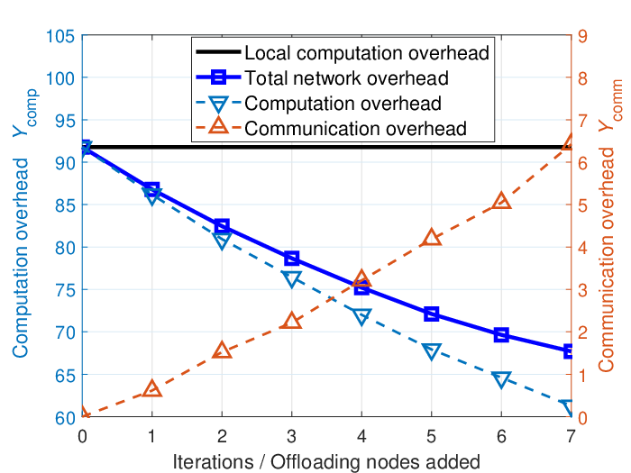
Our next experiment assesses the benefit provided by each offloading node that the greedy algorithm adds in the efficient alternate optimization. Specifically, Fig. 8 shows the change in overhead as more data streams are added for offloading in Algorithm 4, for , , and . We show the evolution of the communication overhead , the computation overhead , and the total overhead . Overall, we see that the total network overhead is decreasing at each iteration, which is consistent with the operation of the greedy algorithm. This is obtained by trading an increase in communication overhead for a more substantial decrease in computation overhead. The algorithm successively exploits low-cost opportunities for offloading from resource constrained to resource-rich nodes, until such opportunities are no longer cost-effective. In this case, 23% of the nodes (7 out of 30) become offloading nodes by the time the algorithm terminates.
V-D Varying Interference Management Resources
Our next experiments assess the communication overhead reduction obtained by our methodology from leveraging interference management resources. When the number of subchannels and number of antennas are limited, we expect that communication overhead will be higher due to decreasing transmission data rates from inter-channel interferences. Fig. 8 shows the effect of on for both the efficient alternate optimization and the baseline using WMMSE, when and there are devices. We see that the total communication overhead decreases as the number of subchannels increases because more subchannels enable avoiding interferences by allocating non-overlapping subchannels to different data streams. Moreover, the efficient alternate optimization with MCOB gives better performance than that with WMMSE – with improvements of roughly 37% for each choice of – because MCOB is designed to minimize the total communication overhead, while WMMSE minimizes only the total communication time.
Fig. 8 shows the effect on communication overhead as more antennas are employed for and . With a limited number of subchannels available (), the beamforming strategy plays a significant role in communication overhead reduction. As increases, our methodology suppresses the interference further due to the increased spatial degrees of freedom. The gap in communication overhead between the efficient alternate optimization with MCOB vs. WMMSE increases with more antennas, reaching roughly a 43% improvement.


V-E Varying Time/Energy Optimization Importance
We are also interested in the impact of the importance placed on time vs. energy in the total network overhead optimization. Fig. 11 demonstrates the effect of the overhead demand factor on the total time delay and energy consumption incurred, aggregating all tasks and over both communication and computation overhead components, for , , and . The individual time delay and energy consumption incurred by each task for different is provided in Appendix D-B. The results in Fig. 11 are consistent with design of the optimization objective: compared to the case of all local computation, total time is reduced the most (36%) when , while more energy reduction (61%) is achieved when . This experiment confirms that the objective can be adjusted according to the tradeoff importance requirement of a specific use case.
Now, we consider the communication overhead optimization to evaluate the performance of MCOB, according to different values of . Fig. 11 shows total communication overhead as varies from 0 to 1 with MCOB and WMMSE, for , , and . When is small, the performances of MCOB and WMMSE are almost identical, as the emphasis is on completion time minimization; in other words, WMMSE is a special case of MCOB for . Since WMMSE does not factor in energy consumption minimization, at any value of , MCOB shows a substantial improvement compared to WMMSE. This emphasizes the importance of considering both time delay and energy consumption as components of the overhead model. Note that the communication overhead of WMMSE increases linearly as increases. This is because the values of and in (20) are constant as a result of WMMSE, and is larger than in this specific D2D scenario. Additionally, the achievable communication overhead by MCOB drops as increases beyond . This is also due to the specific D2D scenario being considered: in (20), as a result of MCOB, the value of (in Joules) is further reduced than (in seconds) as increases.
V-F Varying the Number of Nodes
In this experiment, we compare the total network overhead obtained by efficient alternate optimization and the three baselines as the size of the D2D network changes. Fig. 11 plots as increases for and . Compared to local computation, the other three schemes each yield significant reduction in the total network overhead due to the benefit of offloading. Furthermore, the offloading-enabled methods scale better as the size of the network increase: the performance gap widens and the improvement of the efficient alternate optimization stays around 20% to 30% consistently. With more nodes, there are offloading opportunities, leading to more overhead reduction.
In comparing the offloading-enabled methods, we note that the efficient alternate optimization consistently outperforms the equal CPU allocation and WMMSE baselines (by 7% and 6%, respectively), which are partially optimized solutions. This emphasizes the importance of considering a joint optimization of communication and computation resources to obtain the lowest overhead in an environment of heterogeneous wireless devices. The equal CPU allocation baseline is a lower complexity algorithm, however, given it does not solve the CPU optimization problem. This could be a necessary tradeoff if optimization speed is critical, which depends on the timescale at which the solver is employed in practice. We also provide a comparison between the theoretical and observed computational complexity of our method in Appendix D-A.
VI Conclusion and Future Work
In this paper, we proposed a novel optimization methodology that minimizes the total network overhead required to process a set of tasks in wireless D2D edge networks. Our optimization model consists of several computation and communication resources including topology configuration, CPU allocations, subchannel allocations, and beamforming design for MIMO transmitters and receivers. Given that the problem is a non-convex MIP, we proposed two methods to solve it: semi-exhaustive search optimization and efficient alternate optimization. In analyzing the optimality and computational complexity of the proposed methods, we showed that the semi-exhaustive search can be regarded as a best effort for optimality, while the efficient alternate optimization has much smaller computational complexity. Through our numerical experiments, we showed the total network overhead can be reduced significantly by leveraging offloading opportunities to resource-rich nodes in D2D networks. Further, in comparison with solutions that only optimize a subset of the variables, our results showed that joint communication and computation resource optimization is critical to obtaining the highest reductions in network overhead.
There are several potential avenues of future work. First, while we have focused on tasks generated in a single time period, dynamic task generation at nodes can also be considered. This can be accomplished by augmenting our methodology with a stochastic optimization that models task generation over a long-term time horizon. Second, while we have focused on centralized control for optimizing distributed data processing, it will be desirable to decentralize this optimization in certain settings. One possibility is to investigate a fully distributed implementation of Algorithm 3, where each node solves its local beamforming and resource design sub-problems based on information provided by adjacent neighbors. Lastly, our overhead model can be extended to include components outside of data transmission and processing, e.g., waiting latency, handover latency, and latency of receiving the processed data result back at the origin.
References
- [1] J. Kim, T. Kim, M. Hashemi, C. G. Brinton, and D. J. Love, “Joint optimization of signal design and resource allocation in wireless D2D edge computing,” in IEEE Conf. Comput. Commun., 2020, pp. 2086–2095.
- [2] M. Chiang and T. Zhang, “Fog and IoT: An overview of research opportunities,” IEEE Internet Things J., vol. 3, no. 6, pp. 854–864, 2016.
- [3] C. Yao, X. Wang, Z. Zheng, G. Sun, and L. Song, “Edgeflow: Open-source multi-layer data flow processing in edge computing for 5G and beyond,” IEEE Network, vol. 33, no. 2, pp. 166–173, 2019.
- [4] X. Yang, Z. Chen, K. Li, Y. Sun, N. Liu, W. Xie, and Y. Zhao, “Communication-constrained mobile edge computing systems for wireless virtual reality: Scheduling and tradeoff,” IEEE Access, vol. 6, pp. 665–677, 2018.
- [5] R. Schmoll, S. Pandi, P. J. Braun, and F. H. P. Fitzek, “Demonstration of VR / AR offloading to mobile edge cloud for low latency 5G gaming application,” in IEEE Consumer Commun. Netw. Conf., 2018.
- [6] K. Sultan, H. Ali, and Z. Zhang, “Big data perspective and challenges in next generation networks,” Future Internet, vol. 10, no. 7, 2018.
- [7] Cisco, “Cisco visual networking index: Forcast and trends, 2017-2022,” 2019.
- [8] X. Chen, L. Jiao, W. Li, and X. Fu, “Efficient multi-user computation offloading for mobile-edge cloud computing,” IEEE/ACM Trans. Netw., vol. 24, no. 5, pp. 2795–2808, 2015.
- [9] H. Q. Le, H. Al-Shatri, and A. Klein, “Efficient resource allocation in mobile-edge computation offloading: Completion time minimization,” in IEEE Int. Symp. Inf. Theory, 2017, pp. 2513–2517.
- [10] N. Naderializadeh and M. Hashemi, “Energy-aware multi-server mobile edge computing: A deep reinforcement learning approach,” in Asilomar Conference on Signals, Systems, and Computers, 2019.
- [11] M. Chen and Y. Hao, “Task offloading for mobile edge computing in software defined ultra-dense network,” IEEE J. Sel. Areas Commun., vol. 36, no. 3, pp. 587–597, 2018.
- [12] J. Zhang, X. Hu, Z. Ning, E. C.-H. Ngai, L. Zhou, J. Wei, J. Cheng, and B. Hu, “Energy-latency tradeoff for energy-aware offloading in mobile edge computing networks,” IEEE Internet Things J., vol. 5, no. 4, pp. 2633–2645, 2017.
- [13] T. T. Nguyen, L. Le, and Q. Le-Trung, “Computation offloading in MIMO based mobile edge computing systems under perfect and imperfect CSI estimation,” IEEE Trans. Serv. Comput., 2019.
- [14] S. Sardellitti, G. Scutari, and S. Barbarossa, “Joint optimization of radio and computational resources for multicell mobile-edge computing,” IEEE Trans. Signal Inf. Process. Netw., vol. 1, no. 2, pp. 89–103, 2015.
- [15] S. Barbarossa, E. Ceci, M. Merluzzi, and E. Calvanese-Strinati, “Enabling effective mobile edge computing using millimeterwave links,” in IEEE Conf. Commun. Workshops, 2017, pp. 367–372.
- [16] J. Liu, P. Li, J. Liu, and J. Lai, “Joint offloading and transmission power control for mobile edge computing,” IEEE Access, vol. 7, pp. 81 640–81 651, 2019.
- [17] C. Wang, F. R. Yu, C. Liang, Q. Chen, and L. Tang, “Joint computation offloading and interference management in wireless cellular networks with mobile edge computing,” IEEE Trans. Veh. Technol., vol. 66, no. 8, pp. 7432–7445, 2017.
- [18] X. Cao, F. Wang, J. Xu, R. Zhang, and S. Cui, “Joint computation and communication cooperation for energy-efficient mobile edge computing,” IEEE Internet Things J., 2018.
- [19] X. Diao, J. Zheng, Y. Wu, and Y. Cai, “Joint computing resource, power, and channel allocations for D2D-assisted and NOMA-based mobile edge computing,” IEEE Access, vol. 7, pp. 9243–9257, 2019.
- [20] X. Chen, L. Pu, L. Gao, W. Wu, and D. Wu, “Exploiting massive D2D collaboration for energy-efficient mobile edge computing,” IEEE Wirel. Commun., vol. 24, no. 4, pp. 64–71, 2017.
- [21] H. Xing, L. Liu, J. Xu, and A. Nallanathan, “Joint task assignment and resource allocation for D2D-enabled mobile-edge computing,” IEEE Trans. Commun., 2019.
- [22] Y. He, J. Ren, G. Yu, and Y. Cai, “D2D communications meet mobile edge computing for enhanced computation capacity in cellular networks,” IEEE Trans. Wirel. Commun., vol. 18, no. 3, pp. 1750–1763, 2019.
- [23] Y. Kai, J. Wang, and H. Zhu, “Energy minimization for D2D-assisted mobile edge computing networks,” in IEEE Conf. Commun., 2019.
- [24] N. Hassan, K.-L. A. Yau, and C. Wu, “Edge computing in 5G: A review,” IEEE Access, vol. 7, pp. 127 276–127 289, 2019.
- [25] D. Tse and P. Viswanath, Fundamentals of Wireless Communications. New York: Cambridge University Press, 2005.
- [26] F. Wang, L. Song, Z. Han, Q. Zhao, and X. Wang, “Joint scheduling and resource allocation for device-to-device underlay communication,” in IEEE Wireless Commun. Netw. Conf., 2013, pp. 134–139.
- [27] T. Kim and M. Dong, “An iterative Hungarian method to joint relay selection and resource allocation for D2D communications,” IEEE Wireless Commun. Lett., vol. 3, no. 6, pp. 625–628, 2014.
- [28] L. Wei, R. Q. Hu, T. He, and Y. Qian, “Device-to-device (D2D) communications underlaying MU-MIMO cellular networks,” in Proc. IEEE Glob. Commun. Conf., 2013, pp. 4902–4907.
- [29] M.-H. Han, B.-G. Kim, and J.-W. Lee, “Subchannel and transmission mode scheduling for D2D communication in OFDMA networks,” in IEEE Veh. Technol. Conf. (VTC Fall), 2012.
- [30] J. Zhao, Y. Liu, K. K. Chai, Y. Chen, and M. Elkashlan, “Joint subchannel and power allocation for NOMA enhanced D2D communications,” IEEE Trans. Commun., vol. 65, no. 11, pp. 5081–5094, 2017.
- [31] D. Feng, L. Lu, Y. Yuan-Wu, G. Y. Li, G. Feng, and S. Li, “Device-to-device communications underlaying cellular networks,” IEEE Trans. Commun., vol. 61, no. 8, pp. 3541–3551, 2013.
- [32] X. Lin, R. W. Heath, and J. G. Andrews, “The interplay between massive MIMO and underlaid D2D networking,” IEEE Trans. Wirel. Commun., vol. 14, no. 6, pp. 3337–3351, 2015.
- [33] H. Tang, C. Zhu, and Z. Ding, “Cooperative MIMO precoding for D2D underlay in cellular networks,” in IEEE Conf. Commun., 2013, pp. 5517–5521.
- [34] Q. Shi, M. Razaviyayn, Z.-Q. Luo, and C. He, “An iteratively weighted MMSE approach to distributed sum-utility maximization for a MIMO interfering broadcast channel,” IEEE Trans. Signal Process., vol. 59, no. 5, Sep 2011.
- [35] Z. Zhou, H. Liao, X. Zhao, B. Ai, and M. Guizani, “Reliable task offloading for vehicular fog computing under information asymmetry and information uncertainty,” IEEE Trans. Veh. Technol., vol. 68, no. 9, pp. 8322–8335, 2019.
- [36] Z. Zhou, J. Feng, Z. Chang, and X. Shen, “Energy-efficient edge computing service provisioning for vehicular networks: A consensus ADMM approach,” IEEE Trans. Veh. Technol., vol. 68, no. 5, pp. 5087–5099, 2019.
- [37] Y. Mao, C. You, J. Zhang, K. Huang, and K. B. Letaief, “A survey on mobile edge computing: The communication perspective,” IEEE Commun. Surv. Tutor., vol. 19, no. 4, pp. 2322–2358, 2017.
- [38] S. G. Johnson and M. Frigo, “A modified split-radix FFT with fewer arithmetic operations,” IEEE Trans. Signal Process., vol. 55, no. 1, pp. 111–119, 2006.
- [39] Y. Wen, W. Zhang, and H. Luo, “Energy-optimal mobile application execution: Taming resource-poor mobile devices with cloud clones,” in IEEE Conf. Comput. Commun., 2012, pp. 2716–2720.
- [40] S. Burer and A. N. Letchford, “Non-convex mixed-integer nonlinear programming: A survey,” Surv. Oper. Res. Manag. Sci., vol. 17, no. 2, pp. 97–106, 2012.
- [41] S. M. Ross, Introduction to probability models. Academic press, 2014.
- [42] M. N. Tehrani, M. Uysal, and H. Yanikomeroglu, “Device-to-device communication in 5G cellular networks: challenges, solutions, and future directions,” IEEE Commun. Mag., vol. 52, no. 5, pp. 86–92, 2014.
- [43] L. Pu, X. Chen, J. Xu, and X. Fu, “D2D fogging: An energy-efficient and incentive-aware task offloading framework via network-assisted D2D collaboration,” IEEE. J. Sel. Areas Commun., vol. 34, no. 12, pp. 3887–3901, 2016.
- [44] S. Mumtaz and J. Rodriguez, Smart device to smart device communication. Springer, 2014.
- [45] 3GPP TS 36.211, “LTE: Evolved universal terrestrial radio access (e-utra): Physical channels and modulation,” vol. V14.2.0 Release 14, 2017.
- [46] S.-Y. Lien, S.-L. Shieh, Y. Huang, B. Su, Y.-L. Hsu, and H.-Y. Wei, “5G new radio: Waveform, frame structure, multiple access, and initial access,” IEEE Commun. Mag., vol. 55, no. 6, pp. 64–71, 2017.
- [47] S. G. Larew and D. J. Love, “Adaptive beam tracking with the unscented Kalman filter for millimeter wave communication,” IEEE Signal Process. Lett., vol. 26, no. 11, pp. 1658–1662, 2019.
- [48] M. B. Booth, V. Suresh, N. Michelusi, and D. J. Love, “Multi-armed bandit beam alignment and tracking for mobile millimeter wave communications,” IEEE Commun. Lett., vol. 23, no. 7, pp. 1244–1248, 2019.
- [49] J. Choi, D. J. Love, and P. Bidigare, “Downlink training techniques for FDD massive MIMO systems: Open-loop and closed-loop training with memory,” IEEE J. Sel. Topics Signal Process., vol. 8, no. 5, pp. 802–814, 2014.
- [50] D. J. Love, R. W. Heath, V. K. Lau, D. Gesbert, B. D. Rao, and M. Andrews, “An overview of limited feedback in wireless communication systems,” IEEE J. Sel. Areas Commun., vol. 26, no. 8, pp. 1341–1365, 2008.
- [51] D. J. Love, R. W. Heath, W. Santipach, and M. L. Honig, “What is the value of limited feedback for MIMO channels?” IEEE Commun. Mag., vol. 42, no. 10, pp. 54–59, 2004.
- [52] D. J. Love, R. W. Heath, and T. Strohmer, “Grassmannian beamforming for multiple-input multiple-output wireless systems,” IEEE Trans. Inform. Theory, vol. 49, no. 10, pp. 2735–2747, 2003.
- [53] X. Lyu, H. Tian, C. Sengul, and P. Zhang, “Multiuser joint task offloading and resource optimization in proximate clouds,” IEEE Trans. Veh. Technol., vol. 66, no. 4, pp. 3435–3447, 2016.
- [54] M. Hong and Z.-Q. Luo, “Signal processing and optimal resource allocation for the interference channel,” in Academic Press Library in Signal Processing. Elsevier, 2014, vol. 2, pp. 409–469.
- [55] K. Shen and W. Yu, “Fractional programming for communication systems—part I: Power control and beamforming,” IEEE Trans. Signal Process., vol. 66, no. 10, pp. 2616–2630, 2018.
- [56] S. He, Y. Huang, L. Yang, and B. Ottersten, “Coordinated multicell multiuser precoding for maximizing weighted sum energy efficiency,” IEEE Trans. Signal Process., vol. 62, no. 3, pp. 741–751, 2013.
- [57] J. H. Ferziger, Numerical methods for engineering application. Wiley New York, 1981, vol. 1.
- [58] S. Boyd and L. Vandenberghe, Convex optimization. Cambridge university press, 2004.
- [59] S. Sun, T. S. Rappaport, R. W. Heath, A. Nix, and S. Rangan, “MIMO for millimeter-wave wireless communications: Beamforming, spatial multiplexing, or both?” IEEE Commun. Mag., vol. 52, no. 12, pp. 110–121, 2014.
- [60] J. Zhang, Y. Wu, S. Zhou, and J. Wang, “Joint linear transmitter and receiver design for the downlink of multiuser MIMO systems,” IEEE Commun. Lett., vol. 9, no. 11, pp. 991–993, 2005.
- [61] O. Arnold, F. Richter, G. Fettweis, and O. Blume, “Power consumption modeling of different base station types in heterogeneous cellular networks,” in Future Network & Mobile Summit, 2010.
- [62] S. Y. Seidel and T. S. Rappaport, “914 MHz path loss prediction models for indoor wireless communications in multifloored buildings,” IEEE Trans. Antennas Propag., vol. 40, no. 2, pp. 207–217, 1992.
- [63] C. K. Au-Yeung and D. J. Love, “On the performance of random vector quantization limited feedback beamforming in a MISO system,” IEEE Trans. Wirel. Commun., vol. 6, no. 2, pp. 458–462, 2007.
| Junghoon Kim received the M.S. degree in electrical engineering from Korea Advanced Institute of Science and Technology (KAIST) in 2014. Since 2019, he has worked towards the Ph.D. degree at Purdue University. |
| Taejoon Kim (Senior Member, IEEE) received the Ph.D. degree in electrical and computer engineering from Purdue University in 2011. He is currently an Assistant Professor of electrical engineering and computer science at the University of Kansas (KU). His research interest includes 5G-and-beyond wireless systems and millimeter-wave and terahertz wireless. He was the recipient of the Miller Faculty Award from the KU School of Engineering and The IEEE Communications Society Stephen O. Rice Prize. |
| Morteza Hashemi is an Assistant Professor with the Department of Electrical Engineering and Computer Science at the University of Kansas, Lawrence, Kansas. He received his MSc and PhD degrees in Electrical Engineering from Boston University in 2013 and 2015, respectively. Before joining KU in 2019, he was a postdoctoral researcher and senior lecturer at the Ohio State University. His research interests span the areas of wireless communications, information systems, real-time data networking, and networked cyber-physical systems. |
| Christopher G. Brinton (Senior Member, IEEE) received the Ph.D. degree in electrical engineering from Princeton University in 2016. He is currently an Assistant Professor of electrical and computer engineering with Purdue University. Since joining Purdue University in 2019, he has won several awards including the Seed for Success Award and the Ruth and Joel Spira Outstanding Teacher Award. |
| David J. Love (S’98 - M’05 - SM’09 - F’15) is the Nick Trbovich Professor of Electrical and Computer Engineering at Purdue University. His research interests are in the design and analysis of broadband wireless communication systems, beyond-5G wireless systems, multiple-input multiple-output (MIMO) communications, millimeter wave wireless, software defined radios and wireless networks, coding theory, and MIMO array processing. |
Appendix A Proof of Theorem 1
We first rewrite the problem (44)-(45) to an equivalent form by introducing an auxiliary variable for as
| minimize | (69) | |||||
| subject to | (70) | |||||
| (71) | ||||||
| variables | ||||||
Introducing the Lagrange multipliers and for the two inequality constraints in (70)-(71), we obtain the Lagrange function of the problem (69)-(71) as
| (72) | ||||
where and are denoted as and for simplicity.
Assuming that , , , and are the solutions of the problem (69)-(71), they must satisfy the KKT conditions
| (73) | |||
| (74) | |||
| (75) | |||
| (76) |
where (73)-(76) represent the conditions of stationarity, complementary slackness, primal feasibility, and dual feasibility.
From (40) and (46), and . Furthermore, with the optimal solutions , , and , the inequality is guaranteed. Otherwise, it will drive the value of the objective function in (44) to infinity. Since , the last condition in (73) and first condition in (74) yield
| (77) |
Then, the remaining conditions, i.e., the first three conditions in (73), the second condition in (74), the second condition in (75), and the second condition in (76), are exactly the KKT conditions of the problem below:
| minimize | (78) | |||||
| subject to | (79) | |||||
| variables |
In summary, if , , , and are solutions of the problem (69)-(71), then , , and are solutions of the problem (78)-(79) while simultaneously satisfying (77). The contrary conclusion can be obtained in the opposite direction, which leads to the proof of Theorem 1. If , , and are solutions of the problem (78)-(79) and also simultaneously satisfy the system equations with and in (77), then , , , , and satisfy all of the KKT conditions (73)-(76). This means that , , , and are the solutions of (69)-(71). It follows that , , are optimal solutions of (44)-(45).
Appendix B Proof of Lemma 2
For computational complexity of the two proposed methods, we only need to compare how many combinations of the binary variables and are addressed for optimization. Note that non-integer variables are optimized when the binary variables are given. First, we deal with the computational complexity of the semi-exhaustive search optimization. From the condition (23), each must choose one where . If , we also must choose one from the condition (III-D) where . Then, we have cases for each . This is performed for every , and we get cases. Therefore, we have . Although condition (III-D) can reduce the total number of cases, we consider the worst case scenario for computational complexity.
For the computational complexity of the efficient alternate optimization, a few steps need to be described. As the first iteration of the greedy search, the number of pairs among all nodes is . For each pair, we consider cases from the subchannel allocation condition (III-D). Therefore, we obtain cases at the first iteration. At the second iteration, the transmit candidate set is updated with . Note that . Then, we have cases. At the third iteration, we have or . If the larger case is considered as worst case scenario, total cases will be . This would continue to . We can apply the upper bound and calculate the total combinations approximately as . Therefore, we have .
Appendix C Derivation of the Closed-Form Solution for
To solve problem (52)-(53), for each where , we introduce the Lagrange multiplier for the inequality constraint (53) and obtain the Lagrangian function as
| (80) |
The first-order optimality condition yields
| (81) |
We can obtain the solution as a function of to be
| (82) |
From complementary slackness, dual feasibility, and primal feasibility, the following conditions should be satisfied: , , and . In other words, if , then is the optimal solution. If , then is the optimal solution where should be satisfied for some . In this case, the remaining part is to determine . Using the eigendecomposition and denoting , we can represent as
| (83) |
where denotes the -th element of and denotes the -th diagonal element of . The formula in (83) is a non-increasing function of . Therefore, a finite-interval one-dimensional search method such as the bisection method [57] can be used to determine to satisfy .
Appendix D Additional Experimental Results
D-A Runtime Growth Rate of the Efficient Alternate Optimization
In Fig. 12, we consider the runtime growth rate of the efficient alternate optimization over the number of nodes compared to the theoretical complexity given in Section IV-D. We consider subchannels and antennas. The runtime at is normalized to 1 as a basis, and the growth rate along the number of nodes is plotted. While the growth rate of the worse-case complexity derived in Lemma 2 is , we observe a growth rate is lower than (approximately according to polynomial curve fitting).
Overall, we see that the efficient alternate optimization has polynomial time complexity, which is considered a desirable upper bound in algorithm design. We leave additional improvements in runtime, e.g., to linear time complexity, to future work. In this regard, it may be desirable to have a fully distributed implementation of the efficient alternate optimization. To do so, future work can consider distributed algorithms for the (i) beamforming and (ii) resource design sub-problems. For (i), one can investigate a version of MCOB where each node solves for its own beamformer and combiner, leveraging channel reciprocity, with network information provided by neighbors. For (ii), one can investigate a distributed consensus version of the greedy algorithm, where each node chooses its local candidate for link addition and the nodes collaboratively discover a final decision. The incurred communication overhead from such approaches can also be factored into the overall network overhead optimization.

D-B Example of Task Offloading and Processing


In Fig. 13, we show a more detailed version of the result in Fig. 11, i.e., individual time and energy consumption incurred by each task for different values of through our optimization. The size of each task and available CPU at each node are demonstrated in Fig. 13(a). Intuitively, the nodes () with low CPU and large data size are more likely to offload tasks to other nodes () with high CPU as a result of our optimization. Given the computation and communication resources including subchannels, task size, and available CPU, we apply our efficient alternate optimization methodology for each , with the results summarized in Fig. 13(b)&(c). Fig. 13(b)&(c) break down the time and energy overhead incurred as a result of communication and computation for each task. For , tasks are offloaded to nodes , respectively. For , which increases the emphasis on minimizing energy consumption, tasks are offloaded to nodes , respectively. The rest of the tasks are processed locally.
In order to explore how the time (latency) and energy consumption for processing the data are changed through task offloading, we take a look the specific behavior of task offloaded to node as an example. In Fig. 13(b), for any , we see that the time overhead for task 4, including computation and communication overhead, is greatly reduced as compared to local task processing, because task 4 is offloaded to node 8 which has high CPU. This also leads to increasing the computation time overhead for task 8, because less CPU is allocated to it due to CPU sharing with the offloaded task 4. In Fig. 13(c), the energy consumption for processing task 4 increases as compared to local task processing, because a larger amount of CPU is used to process the offloaded task (at node 8). At the same time, the energy consumption for task 8 decreases because less CPU (at node 8) is now allocated to this task due to CPU sharing. Overall, task offloading is conducted to minimize the optimization objective, which is the weighted sum of total time and energy consumption for processing the data throughout the network. The overall performance in terms of the total time and energy consumption is shown in Fig. 11.
D-C Dynamic Task Generation
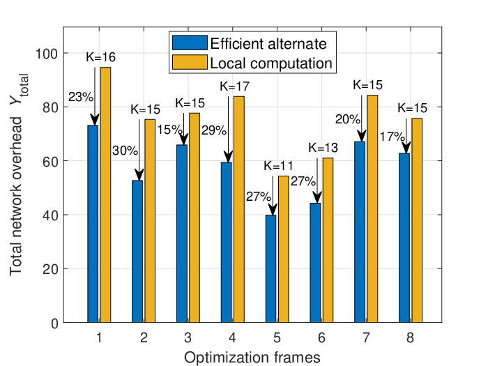
In this experiment, we assess our proposed framework and algorithms under a dynamic task scenario. When a new task is generated at a node, we assume that it is queued until there is a time frame available for it to be processed. Then, the optimization proceeds as a series of frames, where each frame will consider one task from each node in a first in first out (FIFO) manner. Since nodes will not always have tasks in their queue, let denote the set of participating nodes in optimization frame . In Fig. 14, we show a simulation which considers the total network overhead obtained by our efficient alternate optimization algorithm over optimization frames, where the total nodes is and varies from tasks being generated according to a standard queue model [41]. For the queue model, Poisson distributed traffic is considered with task arrival rate (tasks/sec), and the traffic is assumed to be independent across nodes. We consider the period of each optimization frame to be sec. The task size is assumed to be Mbytes for each node. In every optimization frame , the number of participating nodes, , is indicated above the bars in Fig. 14. Overall, the total network overhead is reduced substantially in each time period compared to local computation: between 15% and 30%. This is consistent with our experiments for the non-dynamic case.
The above experiment shows that our framework and algorithms can be applied in the dynamic task setting. Moreover, extensions of the approach we have presented here are noteworthy for future work. For example, optimizing the frame rate over time may provide additional gains in terms of task processing delay and energy efficiency. Doing so would require stochastic optimization to capture dynamic task generation over a long-term time horizon.