Fully Augmented Links in the Thickened Torus
Abstract.
In this article we study the geometry of fully augmented link complements in the thickened torus and describe their geometric properties, generalizing the study of fully augmented links in . We classify which fully augmented links in the thickened torus are hyperbolic, show that their complements in the thickened torus decompose into ideal right-angled torihedra. We also study volume density of fully augmented links in , defined to be the ratio of its volume and the number of augmentations. We prove the Volume Density Conjecture for fully augmented links which states that the volume density of a sequence of fully augmented links in which diagrammatically converge, as defined below, to a biperiodic link, converges to the volume density of that biperiodic link. Furthermore, we show that the complement of a sequence of these links approaches the complement of the biperiodic link as a geometric limit.
1. Introduction
In this paper we study a class of links called fully augmented links. Fully augmented links in are obtained from diagrams of links in as follows. Let be a link in with a given planar link diagram . We encircle each twist region (a maximal string of bigons) of with a single unknotted component called a crossing circle. The complement of the resulting link is homeomorphic to the link obtained by removing all full-twists i.e. pairs of crossings from each twist-region. Therefore, a diagram of the fully augmented link contains a finite number of crossing circles, each encircling two strands of the link. These crossing circles are perpendicular to the projection plane and the other link components are embedded on the projection plane, except possibly for a finite number of single crossings, called half-twists which are adjacent to the crossing circles. See Figure 1.
The geometry of fully augmented link complements in can be explicitly described in terms of an ideal right-angled polyhedral decomposition which is closely related to the link diagram. This geometry has been studied in detail by Adams [3], Agol and D. Thurston [15], Purcell [17] and Cheesbro-Deblois-Wilton [11]. In [10] Champanerkar-Kofman-Purcell studied the geometry of alternating link complements in the thickened torus and described their decompositions into torihedra, which are toroidal analogs of polyhedra. In this paper we combine the methods used to study fully augmented links in and alternating links in the thickened torus to study the geometry of fully augmented link complements in the thickened torus. We generalize many geometric properties of fully augmented links in to those in the thickened torus, , where .
A biperiodic link is an infinite link in with a projection on which is invariant under an action of a two dimensional lattice by translations. The quotient is a link in with a projection on . This projection on is the link diagram of .
Volume density of a link was first introduced by Champanerkar, Kofman and Purcell in [9] as the ratio of its hyperbolic volume, and its crossing number, . In [9] and [10] they studied volume densities of sequences of alternating links in which diagrammatically converge to two specific biperiodic links called the square weave and the triaxial link. They proved that volume density of such a sequence of alternating links converges to that of the corresponding biperiodic link. In general, they conjectured the following:
Conjecture 1.1.
(Volume Density Conjecture [10]) Let be any biperiodic alternating link with alternating quotient link . Let be a sequence of alternating hyperbolic links which Følner converges to . Then
Definition 1.2.
A fully augmented biperiodic link is a fully augmented infinite link in with a projection on which is invariant under an action of a two dimensional lattice by translations. The quotient is a fully augmented link in with a projection on .
We define the volume density of a fully augmented link in (with or without half-twists) to be the ratio of its volume and the number of augmentations. We similarly define volume density of fully augmented links in the thickened torus. Using the geometry of fully augmented link complements in studied previously and our results on the geometry of fully augmented link complements in the thickened torus, we prove the Volume Density Conjecture for fully augmented links.
In Section 2 we classify hyperbolic fully augmented links in the thickened torus.
Theorem 2.11.
Let be a link in with a weakly prime, twist-reduced cellular link diagram . Let be a link obtained by fully augmenting . Then decomposes into two isometric totally geodesic right-angled torihedra, and hence is hyperbolic.
Remark 1.4.
Augmented link diagrams are link diagrams obtained by adding crossing circles to some of the twist sites of a given link diagram and are different from fully augmented links. It was proved in [14] that augmented links in the thickened torus are hyperbolic. A generalization to thickened surfaces was also proved in [12]. Theorem 2.11 above gives a much stronger result for fully augmented links as it describes the right-angled geometry of the complement and uses very different proof techniques than [14] and [12]. The decomposition of the link in Theorem 2.11 into right-angled torihedra (see Definition 2.6) is very important for Theorem 3.20 which investigates limit points of volume densities of fully augmented links.
In Section 3 we discuss volume density and the volume density spectrum of fully augmented links in and give many examples. In Section 3.2 we define Følner convergence for fully augmented links and prove the volume density conjecture for fully augmented links. Følner convergence for links was first defined in [9] for alternating links, we adapt the definition of Følner convergence in this paper for sequences of fully augmented links.
Theorem 3.20.
Let be a biperiodic fully augmented link with quotient link . Let be a sequence of hyperbolic fully augmented links in such that Følner converges to geometrically. Then
where denoted the number of augmentations of a fully augmented link .
As an application in Corollary 3.23 we show that the end point of the volume density spectrum of fully augmented links in is a limit point, by constructing a sequence of hyperbolic fully augmented links in which Følner converge everywhere to a fully augmented biperiodic link whose volume density is .
Acknowledgements I would like to thank my advisor Abhijit Champanerkar for guidance in this paper. I would also like to thank Ilya Kofman and Jessica Purcell for helpful conversations in regards to this project.
2. Hyperbolicity of Fully Augmented Links in the Thickened Torus and Volume Bounds
To define fully augmented links in the thickened torus we first need to define twist-reduced diagrams for links in . Howie-Purcell defined twist-reduced diagrams for links in thickened surfaces in [13]. However for links in the thickened torus we can also define twist-reduced diagrams using the biperiodic link diagram in :

Definition 2.1.
A twist region in the biperiodic link diagram is a maximal string of bigons, or a single crossing. A twist region in the link diagram is a quotient of a twist region in .
A biperiodic link is called twist-reduced if for any simple closed curve on the plane that intersects transversely in four points, with two points adjacent to one crossing and the other two points adjacent to another crossing, the simple closed curve bounds a subdiagram consisting of a (possibly empty) collection of bigons strung end to end between these crossings. See Figure 2. We say is twist-reduced if it is the quotient of a twist-reduced biperiodic link.

Definition 2.2.
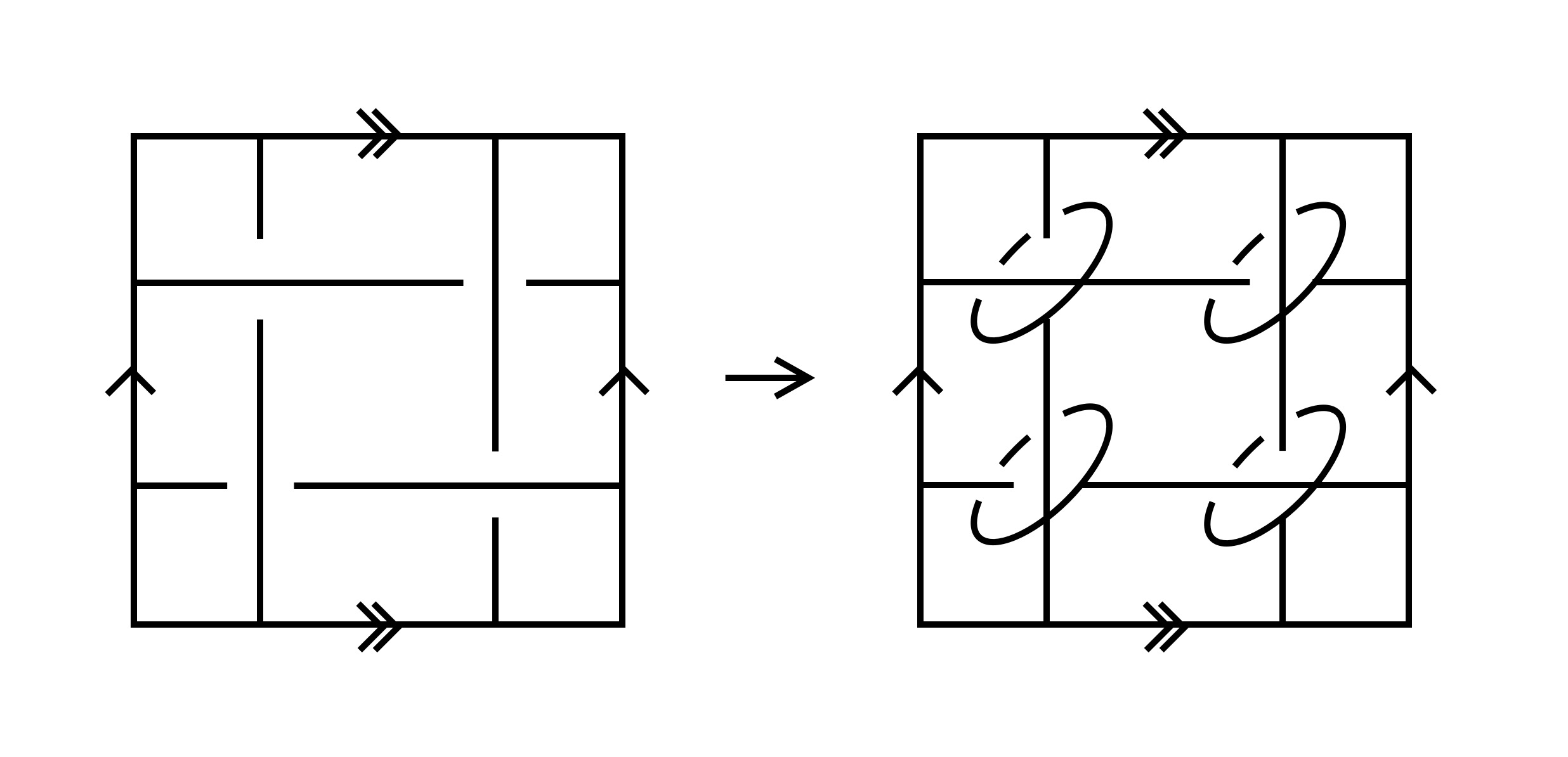
A fully augmented link diagram in is a diagram of a link that is obtained from a twist-reduced diagram in as follows: (1) augment every twist region with a circle component, called a crossing circle (2) get rid of all full twists. See Figure 3. A fully augmented link in is a link which has a fully augmented link diagram in .
Remark 2.3.
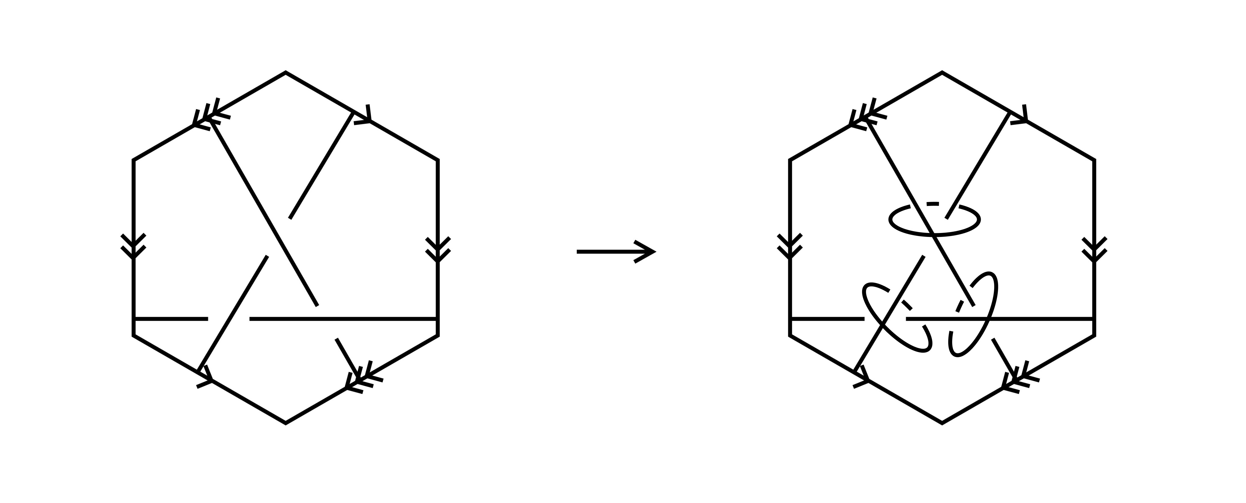
For fully augmented links in , depending on the parity of the number of crossings in a twist region the fully augmented link may or may not have a half-twist at that crossing circle. See the third figure from the left in Figure 1. Similarly depending on the parity of the number of crossings at a twist region a fully augmented link in the thickened torus may or may not have a half-twist at that crossing circle.
 |
|
| (a) | |
 |
|
| (b) |
Definition 2.4.
A graph on the torus is cellular if its complement is a collection of open disks.
Torihedra were first defined in [10] and play the role of polyhedra in polyhedral decompositions of link compliments in e.g. it is proved in [10] that a complement of a link in the thickened torus decomposes into torihedra. Here we recall the definition of a torihedron:
2.1. Torihedral decomposition
Definition 2.5.
A torihedron is a cone on the torus, i.e. , with a cellular graph on . The edges and faces of are called the edges and faces of the torihedron. An ideal torihedron is a torihedron with the vertices of and the vertex removed. Hence, an ideal torihedron is homeomorphic to with a finite set of points (ideal vertices) removed from . The graph is called the graph of the torihedron.
Definition 2.6.
An angled torihedron is a torihedron with an angle assignment on each edge of the graph of the torihedron. An assignment of angle on each edge is called a right-angled torihedron.
Proposition 2.7.
Let be a fully augmented link in , then there is a decomposition of the link complement into two combinatorially isomorphic torihedra such that:
- (1)
The faces of each torihedron can be checkerboard colored such that the shaded faces are triangular and arise from the bow-ties corresponding to crossing circles;
- (2)
The graph of each torihedron is 4-valent.
Proof. We follow the cut-slice-flatten construction described in [15]. Let be a fully augmented link in . We begin by assuming that there are no half twists, the crossing circles are lateral to , and the components of that are not crossing circles lie flat on . There are twice punctured disks bounded by the crossing circles which are perpendicular to the projection plane.
 |
 |
 |
 |
| (a) | (b) | (c) | (d) |
- (1)
Cut along the projection surface into two pieces. This cuts each of the twice-punctured disks bounded by a crossing circle in half. See Figure 4(b).
- (2)
For each of the two pieces resulting from Step 1, slice the middle of the halves of twice-punctured disks and flatten the half disks out. See Figure 4(c).
- (3)
Collapse strands of the link and parts of the augmented circles to ideal vertices in each of the two pieces. See Figure 4(d).
It follows from Steps (1), (2) and (3) that each piece of the decomposition is homeomorphic to with the same graph on with vertices deleted. Hence decomposes into two identical ideal torihedra.
After Step (2) the cut-sliced-flattened half-disks become a hexagon with an edge in the middle corresponding to the strand of the half of a crossing circle. Upon collapsing the crossing circle this becomes a bow-tie. See Figures 4(c) and 4(d). Each vertex of the graph is four-valent since it is shared by two triangles of either two different bow-ties or one bow-tie. Again by construction each edge is shared by a triangle of a bow-tie and a polygon that does not come from a bow-tie see Figure 4(d). Hence we can shade each triangle of the bow-tie to get a checkerboard coloring on the graph of the torihedron such that the shaded faces are bow-ties.
The two torihedra are glued together as follows: the white faces are glued to the corresponding white faces, and the bow-ties are glued as shown in Figure 6(a).
In the case when there is a half-twist at a crossing circle, we split the whole twice-punctured disk into two copies, and flip one of the disks to remove the half-twist. This only affects the gluing of faces of the torihedra. Hence if there are half-twists, then we get the same torihedra but with a different gluing pattern on the bow-ties as shown in Figures 5 and 6(b). ∎

 |
 |
| (a) | (b) |
Definition 2.8.
For a fully augmented link in the thickened torus the decomposition of described above is called the bow-tie torihedral decomposition of . We call the graph of the torihedra the bow-tie graph of and denote it as .
Lemma 2.9.
Let be a hyperbolic fully augmented link in . The following surfaces are embedded totally geodesic surfaces in the hyperbolic structure on the link complement.
- (1)
Each twice-punctured disk bounded by a crossing circle,
- (2)
Each connected component of the projection surface.
Proof. (1) The disk bounded by a crossing circle is punctured by two arcs of the link diagram lying on the projection plane. Adams [2] showed that any incompressible twice-punctured disk properly embedded in a hyperbolic 3-manifold is totally geodesic. Hence it suffices to show that is incompressible. Let be a hyperbolic fully augmented link in . Since , where is the Hopf link, is a hyperbolic link in .
Suppose there is a compressing disk with with . Since is an essential closed curve on , it must encircle one or two punctures of . Suppose it encircles only one puncture. This means that the union of and the disk bounded by inside the closure of forms a sphere in met by the link exactly once. This is a contradiction to the generalized Jordan curve theorem. Hence must bound a twice-punctured disk on . This means is a boundary compressing disk for the crossing circle, contradicting the boundary irreducibility of .
(2) Notice that the reflection through the projection surface
() preserves the link complement, fixing the plane
pointwise. Then it is a consequence of Mostow-Prasad rigidity that
such a surface must be totally geodesic.
(See Lemma 2.1 in [17]) ∎
2.2. Hyperbolicity
Definition 2.10.
Let be a biperiodic link with diagram . We say is prime if whenever a disk embedded in meets transversely in exactly two edges, then the disk contains a simple edge of the diagram and no crossings. See Figure 7.
A diagram of a link in , denoted is weakly prime if is a quotient of a prime biperiodic link diagram in

Theorem 2.11.
Let be a link in with a weakly prime, twist-reduced cellular link diagram . Let be a link obtained by fully augmenting . Then decomposes into two isometric totally geodesic right-angled torihedra, and hence is hyperbolic.
The proof of Theorem 2.11 relies on a result about the existence of certain circle patterns on the torus due to Bobenko and Springborn [6]. We use similar ideas from [10] to prove Theorem 2.11
Theorem 2.12.
[6]. Suppose is a 4-valent graph on the torus , and is a function on edges of that sums to around each vertex. Let denote the dual graph of . Then there exist a circle pattern on with circles circumscribing faces of (after isotopy of ) and having exterior intersection angles , if and only if the following condition is satisfied:
Suppose we cut the torus along a subset of edges of , obtaining one or more pieces. For any piece that is a disk, the sum of over the edges in its boundary must be at least , with equality if and only if the piece consists of only one face of (only one vertex of ).
The circle pattern on the torus is uniquely determined up to similarity.
Proof of Theorem 2.11. Decompose
into two torihedra using Proposition 2.7. Let
be the bow-tie graph on . Assign angles
for every edge in . We now verify
the condition of Theorem 2.12. This will prove the
existence of an orthogonal circle pattern
(circle pattern whose angle at the intersection of any two circles is orthogonal)
circumscribing the faces of
.
Let be a loop of edges of enclosing a disk
. Suppose intersects edges of transversely. Let
denote the number of vertices of that lie in , and let
denote the number of edges of inside disjoint from
. Because the vertices of are 4-valent and since the
edges inside which are disjoint from get counted twice for
each of its end vertex, . This implies is
even. Since is weakly prime and is made up of edges dual to
this implies . Since is even, . Hence
the sum of the angles for all edges of must be at least .
We now show that this is an equality if and only if
consists of one face of , i.e. encloses only one
vertex. Suppose that the sum
. Since
, for every , and is even,
. Moreover
Hence encloses more than one vertex.
Conversely, let
. This implies .
Let the edges of be for with incident to vertices and and . Let the faces dual to be . Without loss of generality, let be a shaded triangular face. Since is checkerboard colored, is also shaded triangular face.
Suppose then the edge must enter a white face which has empty intersection with . See Figure 8(a).
Since the bowties correspond to crossing circles, see Figure 9(a), the loop gives a loop which intersects . At the vertex , which is in the shaded bowtie, at least one of the edges incident to has to intersect . If only one edge at intersects , since bounds a disk, only one edge at intersects , giving the case shown in Figure 9(b). Similarly, If both edges incident to intersect , since bounds a disk, then the same is true for both edges incident at , giving the case shown in Figure 9(c). If intersects two strands of as in Figure 9(b), since bounds a disk, this contradicts the weakly prime condition of . If intersects two strands on each side as in Figure 9(c), this will contradict twist-reduced condition on .
Therefore . Since both faces are triangles, they can only intersect in a vertex. This implies that encloses a single vertex. See Figure 8(b).
 |
 |
| (a) | (b) |
 |
 |
 |
| (a) | (b) | (c) |
Now, since we showed that is a graph on the torus which satisfies the conditions of Theorem 2.12 there exists an orthogonal circle pattern on the torus with circles circumscribing the faces of . Since a white face of the decomposition intersects any other white face only at ideal vertices, the circles which circumscribe the white faces create a circle packing, where the points of tangency are those corresponding to the associated ideal vertices. Since is 4-valent and every edge has been assigned an angle of , the circles of the shaded faces meet orthogonally.
Lifting the circle pattern to the universal cover of the torus defines an orthogonal biperiodic circle pattern on the plane. Considering the plane as a part of the boundary of , this circle pattern defines a right-angled biperiodic ideal hyperbolic polyhedron in . The torihedron of the decomposition of is the quotient of by which is now realized as a right-angled hyperbolic torihedron. It follows from Theorem 1.1 of [13] that is hyperbolic.∎
Remark 2.13.
Adams [3] proved that fully augmented link complements in are hyperbolic. We have proved an analogous result for fully augmented link complements in . Our method of finding an orthogonal circle pattern which circumscribed the faces of the bow-tie graph can also be applied to the case of fully augmented links in . In this we have to use Andreev’s theorem [19] to ensure a totally geodesic right-angled polyhedra.
2.3. Volume bounds
We show that a hyperbolic fully augmented link with crossings in the thickened torus have an upper volume bound of . In the next section we show volume density convergence of fully augmented links. This means if we can find a link in the thickened torus whose volume is exactly the corresponding biperiodic link will have volume density . We will use this to show that an end point of the volume density spectrum of fully augmented links can be obtained as a limit.
Proposition 2.14.
Let be a hyperbolic fully augmented link with crossing circles. Then
where is the volume of a regular ideal octahedron and is the volume of a regular ideal tetrahedron.
Proof. We will first prove the lower bound. By work of Adams [3], the volume of the complement of in agrees with that of the fully augmented link with no half-twists. This means a lower volume bound for the complement of in with half-twists will be a lower volume bound of the fully augmented link with no half-twists. Hence we will assume has no half-twists and obtain a lower bound for .
Cut along the reflection plane , dividing it into two isometric hyperbolic manifold. The boundary of each of these are the regions of on the projection surface with punctures for the crossing circles. By Lemma 2.9 these regions are geodesic. Hence cutting along the projection surface divides into isometric hyperbolic manifolds with totally geodesic boundary.
Miyamoto showed that if is a hyperbolic 3-manifold with totally geodesic boundary, then vol() [16], with equality exactly when decomposes into regular ideal octahedra. In our case, the manifold consists of two copies of with half-annuli removed for half the crossing circles. For every half a crossing circle removed, we are removing one edge and two vertices. Hence for each crossing circle removed the Euler characteristic changes by . Since there are crossing circles the Euler characteristic would be for each half-cut . The lower bound now follows.
We now prove the upper bound. The torihedral decomposition of the link complement gives a decomposition into two identical ideal torihedra. Every triangular shaded face which comes from a bowtie corresponding to a crossing circle gives a tetrahedron when coned to the ideal vertex on each torihedra. Since there are crossing circles, this gives bowties, hence triangular shaded faces and hence tetrahedra. The cones on the white faces in each torihedra can be glued to make bipyramids on the white faces. These bipyramids can then be stellated into tetrahedra. Hence the the number of tetrahedra coming from stellated bipyramids equals the number of edges of all the white faces. Since an edge of a white face is shared with an edge of a black triangle, this equals the number of edges of the torihedral graph, which has edges. Hence the bipyramids on the white faces decompose into tetrahedra. Thus total count of tetrahedra is . Since the volume of an ideal tetrahedron is bounded by the volume of the regular ideal tetrahedron , the upper bound now follows. ∎
Remark 2.15.
In Proposition 3.7 below we show that our upper bound is sharp by showing that the fully augmented square weave achieves the upper bound.
3. Volume density convergence conjecture
3.1. Volume density and its spectrum
In this section we discuss volume density of fully augmented links in , its spectrum and asymptotic behavior. Champanerkar, Kofman and Purcell [9] defined volume density of a hyperbolic link in as the ratio of the volume of the link complement to its crossing number, and studied the asymptotic behavior of the volume density for sequences of alternating links which diagrammatically converge to a biperiodic alternating link.
For a hyperbolic link in , let denote the hyperbolic volume of . In this section we assume that all links discussed below are hyperbolic.
Definition 3.1.
Let be a fully augmented link in with or without half-twists. The volume density of is defined to be the ratio of the volume of and the number of augmentations, i.e. where is the number of augmentations of the link . We similarly define the volume density of a fully augmented link in .
Remark 3.2.
Adams [3] showed that the volume of an augmented link with a half-twist at the crossing circle of the augmentation is equal to the volume without a half-twist. However fully augmented links with and without half-twists have different crossing numbers. Hence in our definition above we divide by the number of augmentations rather than the number of crossings.
Remark 3.3.
For a fully augmented link without half-twist the crossing number of the diagram is . Thus the volume density of such a fully augmented link is related to the volume density of as defined in [9] by a factor of .
Throughout this section and the next we consider fully augmented links without half-twists.
Example 3.4.
The Borromean rings has and , hence the volume density .
Definition 3.5.
The volume density spectrum of fully augmented links in is defined as fully augmented link in .
Proposition 3.6.
The volume density spectrum .
Proof. Let be a fully augmented link then by Proposition 3.8 of [17] the volume of is at least . Since is hyperbolic, , which implies that the volume density
Since volume density of the Borromean Rings is , the lower bound is realized. Agol and D. Thurston [15] showed that . Hence the the volume density of is at most . ∎
 |
 |
 |
 |
| (a) | (b) | (c) | (d) |
We show below that occurs as a volume density of the fully augmented square weave. Let denote the fully augmented square weave as in Figure 10(b).
Proposition 3.7.
Proof. A four-fold quotient of as shown in Figure 10(d) was studied in [7]. The authors proved that the volume of this link complement in the thickened torus is . Hence , and its volume density is . ∎
Remark 3.8.
The quotient of as in Figure 10(d) has the same volume as that of a quotient of a triaxial link which is not a fully augmented link, see Figure 3(a). However the two links are not the same as they have different number of cusps. The triaxial link has 5 cusps, 3 cusps from each link component in the thickened torus and 2 cusps from each link component of the Hopf Link. Whereas, the quotient of in Figure 10(d) has 4 cusps, 2 from each component of the link in the thickened torus (which includes the crossing circle) and 2 cusps from each link component of the Hopf Link.
3.2. Følner convergence
The volume density of the fully augmented square weave is . We will prove below that is also a limit point of the by investigating the asymptotic behavior of volume density of a sequence of fully augmented links in which diagrammatically converge to the biperiodic fully augmented square weave, as defined below. We use the the notion of Følner convergence, which was first introduced in [9]. We begin by modifying the definition of Følner convergence given in [9].
In [9] the authors used the Tait graph (checkerboard graph) of alternating links to define Følner convergence. We will use bow-tie graphs to define Følner convergence for fully augmented links, see Definition 2.8 and Proposition 2.2 of [17].
|
 |

 |
| (a) | (b) | (c) |
|
|

 |
| (a) | (b) | (c) |


Definition 3.9.
Let be a biperiodic fully augmented link. We will say that a sequence of fully augmented links in Følner converges almost everywhere geometrically to , denoted by , if the respective bow-tie graphs and satisfy the following: there are subgraphs such that
- (1)
, and ,
- (2)
, where denotes the number of vertices, and consists of the vertices of that share an edge in with a vertex not in ,
- (3)
, where represents copies of the fundamental domain for the lattice such that ,
- (4)
.
Remark 3.10.
The number 3 appears in the denominator in the last condition for the definition of Følner convergence because the number of vertices of the bow-tie polyhedron for equals three times the number of augmentations. To see this note that every bow-tie shares two vertices with another bow-tie and hence contributes vertices to the graph. Since each bow-tie corresponds to a crossing circle, the number of vertices of the graph is .
Remark 3.11.
Note that many fully augmented links can have the same bow-tie graph. For example, a fully augmented link with and without half-twists have the same bow-tie graph but different gluing. See Figure 11 and Figure 12. Another example of this is when the bow-tie graphs are same but with different pairing of triangles. See Figure 13 for an example of two links with same bow-tie graphs but different pairings. In our definition above, we are using only the polyhedral graphs but not the pairing information of the bow-ties. Hence we call our Følner convergence geometric. This has the advantage of having many more sequences converging to a given biperiodic fully augmented link.
3.3. Volume Density Conjecture
Conjecture 3.12.
(Volume Density Conjecture) Let be any biperiodic alternating link with alternating quotient link . Let be a sequence of alternating hyperbolic links such that Følner converges to . Then
Champanerkar, Kofman and Purcell proved this conjecture when is the square weave [9] and the triaxial link [8]. by finding upper and lower bounds on such that for a sequence of alternating links , these bounds are equal in the limit. One of the key tools in their proof is the use of right-angled circle patterns. Using the right-angled decomposition of fully augmented link complements in we construct right-angled circle patterns, and use these to prove the Volume Density Conjecture for fully augmented links in .
The idea is as follows: As described in [17] each hyperbolic fully augmented link complement in can be decomposed into two right-angled ideal polyhedra which are described by a right-angled circle pattern. By Theorem 2.11 each torihedra of the bow-tie torihedral decomposition are right-angled described by another right-angled circle pattern on the torus. The lift of this circle pattern is the circle pattern associated to . We show below that when a sequence of fully augmented links converges to , , the circle pattern for converges to infinite circle pattern for . As a consequence we obtain the volume density convergence.
In order to work with circle patterns and convergence of circle patterns, we recall the following definitions from [4]:
Definition 3.13.
A disk pattern is a collection of closed round disks in the plane such that no disk is the Hausdorff limit of a sequence of distinct disks and such that the boundary of any disk is not contained in the union of two other disks.
Definition 3.14.
A simply connected disk pattern is a disk pattern in the plane so that the union of the disks is simply connected.
Let be a disk pattern in . Let be the graph with a vertex for each disk and an edge between any two vertices when the corresponding disks overlap. The graph inherits an embedding in the plane from the disk pattern and we will identify with its plane embedding. A face of is an unbounded component of the complement of in the plane. We can label the edges of with the angles between the intersecting disks.
Definition 3.15.
A disk pattern is called an ideal disk pattern if the labels of edges of are in the interval and the labels around each triangle or quadrilateral in sum to or respectively.
It is clear that ideal disk patterns in correspond to ideal polyhedra in , with the disks corresponding to the faces of the ideal polyhedron.
Definition 3.16.
Let and be disk patterns. Give and the path metric in which each edge has length 1. For disks in and in , we say and agree to generation n if the balls of radius centered at vertices corresponding to and admit a graph isomorphism, with labels on edges preserved.
Definition 3.17.
For a disk in a disk pattern , we let be the geodesic hyperplane in whose boundary agrees with that of . That is, is the Euclidean hemisphere in with boundary coinciding with the boundary of . For a disk pattern coming from a right-angled ideal polyhedron, the planes form the boundary faces of the polyhedron. In this case, the disk pattern is simply connected and ideal, since it corresponds to an ideal polyhedron.
Similarly, for a disk in , with intersecting
neighboring disks , the intersection
is a geodesic in . The
geodesics for on bound an ideal
polygon in . The cone of this polygon to the point at infinity
is denoted by . See Figure 14.


Definition 3.18.
A disk pattern is said to be rigid if has only triangular and quadrilateral faces and each quadrilateral face has the property that the four corresponding disks of the disk pattern intersect in exactly one point.
We will use the following lemma proved by Atkinson in [4].
Lemma 3.19.
[4] Let be an infinite rigid disk pattern. Then there exists a bounded sequence converging to zero so that if is a simply connected, ideal, rigid finite disk pattern containing a disk so that and agree to generation then
Note that the sequence in above Lemma only depends on .
We are now ready to prove:
Theorem 3.20.
(Volume Density Conjecture for fully augmented links) Let be a biperiodic fully augmented link with quotient link . Let be a sequence of hyperbolic fully augmented links in . Then
Proof: Let be the bow-tie torihedron with bow-tie graph of . Let be the infinite polyhedron in which is the biperiodic lift of with its cone vertex taken to be . can be seen to be made up of copies of an embedding of in with its cone vertex taken to be , glued according to the biperiodic lift. Note that since the graph of is the bow-tie graph of , which is toroidal, the graph of is a biperiodic lift of and is isomorphic to the bow-tie graph coming from . Let be the infinite disk pattern coming from the infinite polyhedron . Since is right-angled torihedron, is also right-angled, and hence is a right-angled disk pattern.
Since is a sequence of fully augmented links, each is a fully augmented hyperbolic link in . The bow-tie polyhedron of is a right-angled ideal hyperbolic polyhedron with the same graph as the bow-tie graph . The assumption that the sequence Følner converges almost everywhere geometrically to implies that there are subgraphs which satisfy the conditions of Følner convergence in Definition 3.9. Hence we can embed bow-tie polyhedra of in such that they satisfy the following two conditions: (1) Pick a vertex in to send to infinity, and (2) . We denote this polyhedron in by . First note that . Let denote the number of vertices of . Since is a 4-valent checkerboard graph whose shaded faces are triangles coming from the bow-ties, one for each augmentation, every vertex is shared by two triangles. Hence . Therefore,
Let be the disk pattern of the polyhedron . It follows that is a right-angled, simply connected disk pattern. Since corresponds to a disk pattern arising from a fully augmented link, is rigid (see Definition 3.18, Figure 15). We will now use Følner convergence to relate and .
Let be the set of disks in so that agrees to generation but not to generation with . For every positive integer , let denote the number of faces of with sides that are not contained in and do not meet the point at infinity. By counting vertices we obtain
The term counts the number of vertices that are in but not in . Since all the vertices of the graph are four valent we get a factor of . Hence , and
| (1) |

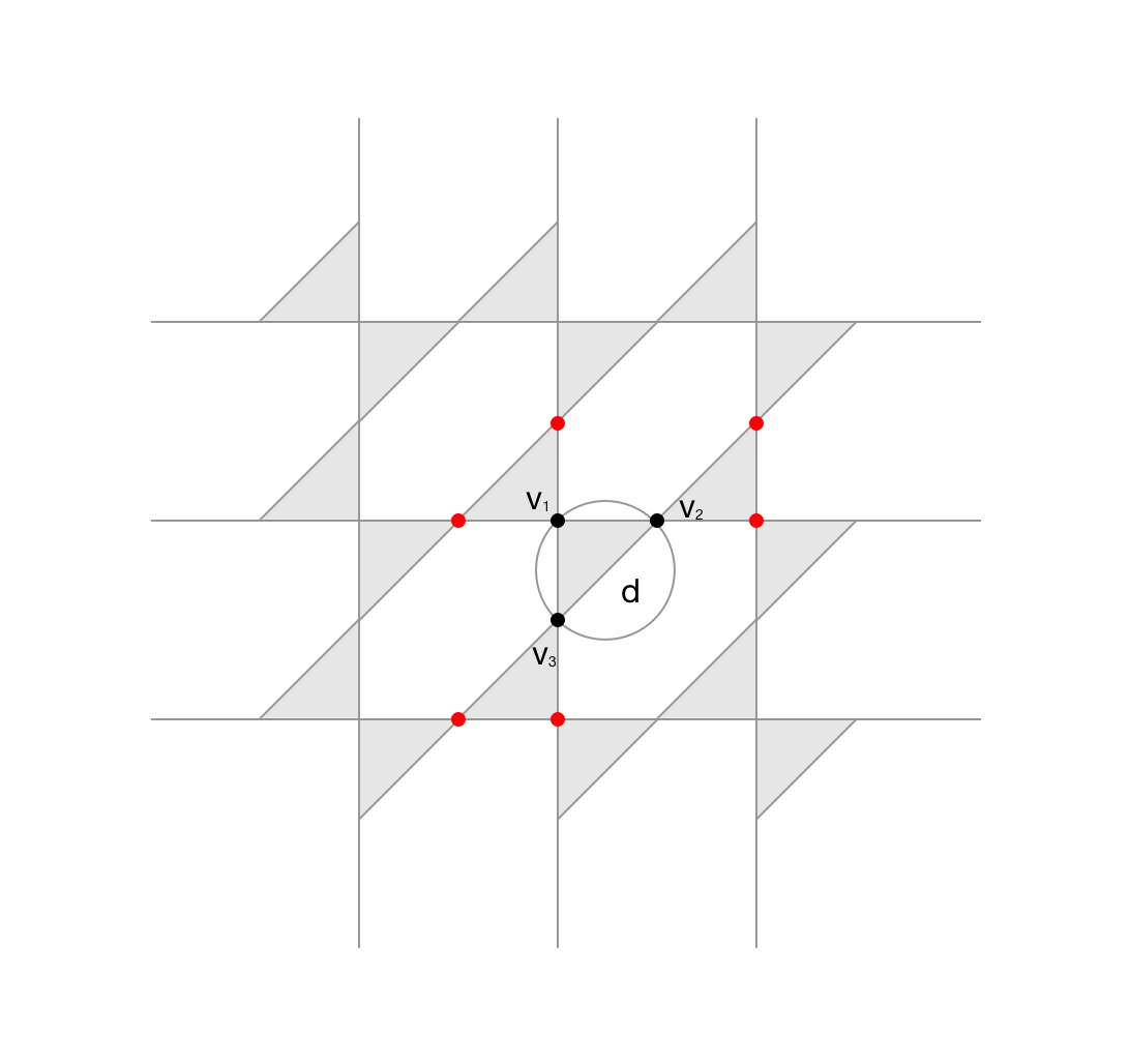
Let and let be the vertices of which lie on the boundary of , see Figure 16. Let denote the ball centered at vertex of radius in the path metric on . It follows from the definition of and the fact that is the planar dual of the graph of the disk pattern (without the vertex corresponding to the unbounded face), implies that but for . Hence the distance from to is i.e. for some for all .
Hence .
Lemma 3.21.
Proof.
We begin by showing that there exists such that for any . By definition of Følner convergence, . Babai [5] showed that the growth rate for almost vertex transitive graphs with one end is quadratic i.e. growth of is quadratic in . Since is a biperiodic 4-valent planar graph, it satisfies the conditions of Babai’s theorem, and hence has quadratic growth rate. By definition, the vertices in are incident to vertices in , hence has linear growth rate in .
Thus, and we obtain
Since , every vertex of lies on a disk in for some and for every disk in there are no vertices in which lie on the disk. Now, by assumption . Hence ∎
Let be the face with sides that is not contained in which does not meet the point at infinity. For each , , where is the the Lobachevsky function defined as
Let denote the sum of the actual volumes of all the cones over the faces , for every integer . Then we have
| (2) |
As mentioned before, every vertex of lies on a disk in for some and for every disk in there are no vertices in which lie on the disk. By assumption . where represents copies of the fundamental domain for the lattice such that .
Since the cone vertex of the torihedron for is at infinity, the disk pattern obtained from taking copies of just extends the disk pattern from one copy of to grid as in Figure 17. The graph for the disk pattern for copies of intersects in , as in Figure 15.
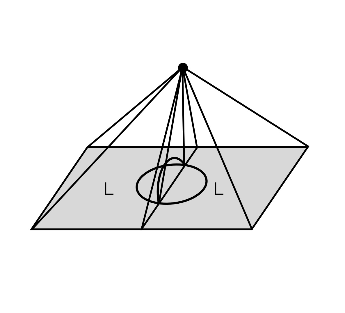
For any face in , let be a positive number such that where is a face in the disk pattern of such that the graph isomorphism between and sends to . Furthermore, we choose so that we can bound the sequence of by a sequence which will converge to zero as in Lemma 3.19.
| (4) |
We divide each term by and take the limit. For the first term of Equation 4, we obtain
From our assumption of the Følner convergence the last condition gives us:
Lemma 3.22.
.
Proof.
Fix any Because there is sufficiently large such that , for . Then is a finite number, say . Since we’ve seen above that and , there exist such that if then and . Then for ,
∎
Now setting we get that the limit of the second term is zero.
Finally, by Equation 1 and Equation 2 we get the third term of Equation 4 equal to zero
Therefore, which means
∎
Recall by we mean the fully augmented square weave link whose quotient is with volume
Corollary 3.23.
Let be any sequence of hyperbolic fully augmented links such that Følner converges everywhere to . Then
∎
References
- [1] Colin Adams, Aaron Calderon, and Nathaniel Mayer. Generalized bipyramids and hyperbolic volumes of alternating -uniform tiling links. Topology Appl., 2020.
- [2] Colin C. Adams. Thrice-punctured spheres in hyperbolic -manifolds. Trans. Amer. Math. Soc., 287(2):645–656, 1985.
- [3] Colin C. Adams. Augmented alternating link complements are hyperbolic. In Low-dimensional topology and Kleinian groups (Coventry/Durham, 1984), volume 112 of London Math. Soc. Lecture Note Ser., pages 115–130. Cambridge Univ. Press, Cambridge, 1986.
- [4] Christopher K. Atkinson. Volume estimates for equiangular hyperbolic Coxeter polyhedra. Algebr. Geom. Topol., 9(2):1225–1254, 2009.
- [5] László Babai. The growth rate of vertex-transitive planar graphs. In Proceedings of the Eighth Annual ACM-SIAM Symposium on Discrete Algorithms (New Orleans, LA, 1997). ACM, New York, 1997.
- [6] Alexander I. Bobenko and Boris A. Springborn. Variational principles for circle patterns and Koebe’s theorem. Trans. Amer. Math. Soc., 356(2):659–689, 2004.
- [7] Abhijit Champanerkar, David Futer, Ilya Kofman, Walter Neumann, and Jessica S. Purcell. Volume bounds for generalized twisted torus links. Math. Res. Lett., 18(6):1097–1120, 2011.
- [8] Abhijit Champanerkar and Ilya Kofman. Determinant density and biperiodic alternating links. New York J. Math., 2(22):891–906, 2016.
- [9] Abhijit Champanerkar, Ilya Kofman, and Jessica S. Purcell. Geometrically and diagrammatically maximal knots. J. Lond. Math. Soc. (2), 94(3):883–908, 2016.
- [10] Abhijit Champanerkar, Ilya Kofman, and Jessica S. Purcell. Geometry of biperiodic alternating links. J. Lond. Math. Soc. (2), 99(3):807–830, 2019.
- [11] Eric Chesebro, Jason DeBlois, and Henry Wilton. Some virtually special hyperbolic 3-manifold groups. Comment. Math. Helv., 87(3):727–787, 2012.
- [12] Darin Li Qiao Li Jacob McErlean Alexander Simons Natalie Stewart Xiwen Wang Colin Adams, Michele Capovilla-Searle. Generalized augmented cellular alternating links in thickened surfaces are hyperbolic, https://arxiv.org/abs/2107.05406 [math.GT], 2021.
- [13] Joshua A. Howie and Jessica S. Purcell. Geometry of alternating links on surfaces. Trans. Amer. Math. Soc., 373(4):2349–2397, 2020.
- [14] Alice Kwon and Ying Hong Tham. Hyperbolicity of augmented links in the thickened torus, https://arxiv.org/abs/2010.1060 [math.GT], 2020.
- [15] Marc Lackenby. The volume of hyperbolic alternating link complements. Proc. London Math. Soc. (3), 88(1):204–224, 2004. With an appendix by Ian Agol and Dylan Thurston.
- [16] Yosuke Miyamoto. Volumes of hyperbolic manifolds with geodesic boundary. Topology, 33(4):613–629, 1994.
- [17] Jessica S. Purcell. An introduction to fully augmented links. In Interactions between hyperbolic geometry, quantum topology and number theory, volume 541 of Contemp. Math., pages 205–220. Amer. Math. Soc., Providence, RI, 2011.
- [18] Jessica S. Purcell. Hyperbolic Knot Theory. Graduate Studies in Mathematics, to appear. American Mathematical Society, Providence, RI, 2020.
- [19] W. P. Thurston. The geometry and topology of three-manifolds. Princeton Univ. Math. Dept. Notes. Available at http://www.msri.org/communications/books/gt3m. [2, 21, 50, 58, 68, 87, 89, 94, 97, 99, 138, 196], 1979.