Many-body chaos and anomalous diffusion across thermal phase transitions in two dimensions
Sibaram Ruidas and Sumilan Banerjee*
Centre for Condensed Matter Theory, Department of Physics, Indian Institute of Science, Bangalore 560012, India * sumilan@iisc.ac.in
August 11, 2026
Abstract
Chaos is an important characterization of classical dynamical systems. How is chaos linked to the long-time dynamics of collective modes across phases and phase transitions? We address this by studying chaos across Ising and Kosterlitz-Thouless transitions in classical XXZ model. We show that spatio-temporal chaotic properties have crossovers across the transitions and distinct temperature dependence in the high and low-temperature phases which show normal and anomalous diffusions, respectively. Our results also provide new insights into the dynamics of interacting quantum systems in the semiclassical limit.
1 Introduction
Chaotic systems are described by a growth rate, the maximum Lyapunov exponent , of perturbation to the initial condition. In recent years, a quantum Lyapunov exponent, and a butterfly velocity for ballistic spread of local perturbation, computed from the out-of-time-order commutator (OTOC) have emerged as important measures for chaos in quantum many-body systems having some well-defined semiclassical limit [1, 2, 3, 4]. In these quantum systems where the Lyapunov exponent can be extracted, it has been perceived as a rate for early-to-intermediate-time thermalization. Here, thermalization refers to the emergence of statistical mechanical description during dynamical evolution of the system. However, it is still controversial [5] whether chaos in isolated interacting classical systems is essential for thermalization.
The recent interest in chaos in quantum many-body systems stems from the proof of a remarkable upper bound, , for [6] and a relation, , between diffusion coefficient , a quantity related to transport, and and in certain strongly interacting systems [7]. Such bounds have been phenomenologically conjectured for transport scattering rate [8, 9], or more conventional relaxation rates extracted from usual time-ordered correlation functions. However, these conjectured bounds have not been concretely established. As a result, even if we set aside the issue of actual role of chaos in thermalization, the temperature () dependence of , and other quantities related to chaos, can serve as a fundamental characterization of phases and phase transition as various chaotic fixed points, like certain non-Fermi liquids and Fermi liquids [10, 11, 12, 13]. The former are highly chaotic with at low temperature, whereas the weakly interacting Fermi liquids show , essentially dictated by quasiparticle decay rate. Motivated by these, here we ask whether many-body chaos can be used to classify phases and finite- phase transitions in classical systems with intrinsic dynamics. An example of such systems is interacting classical Heisenberg spins on a lattice with precession dynamics.
However, typically, chaos is a probe of the short- and intermediate-time behaviour. On the other hand, the long-time dynamical properties of interacting many-body systems, in symmetry broken and unbroken phases, and across phase transitions, are mostly characterized by the properties of the collective low-energy excitations, hydrodynamic and critical modes. How are the short-time chaotic properties of many-body systems related to their long-time dynamics? To address these questions, we look into the connection of chaos with transport, characterized in terms of usual dynamical spin-spin correlations in the spin system.
Classical many-body chaos under Poisson-bracket spin dynamics has been studied in some recent works for various spin models at high [14] and low temperatures [15], as well as across a spin-glass transition in a zero-dimensional spin model [16]. Also, there have been similar studies in other dynamical models like Burgers hydrodynamics [17], and in the classical limit of a relativistic field theory [18]. There are many earlier studies of maximum Lyapunov exponent as well as full Lyapunov spectrum in spin models, molecular systems, and across classical phase transitions [19, 20, 21, 22, 23, 24, 25, 26, 27, 28, 29, 30]. The conventional Lyapunov spectrum analysis, in principle, can reveal the spatiotemporal structure of chaos [31, 32, 33]. However, Lyapunov spectrum analysis typically makes the direct information about the spatial structure somewhat obscure. In this regard, a spatiotemporal correlation function like OTOC [34, 14] provides much more transparent way by explicitly revealing spatial spread of a local perturbation. Thus, in contrast to earlier works [19, 20, 21, 22, 23, 24, 25, 26, 27, 28, 29, 30], using a classical version of OTOC [14], we establish the detailed temperature dependence of both temporal () and spatial () characteristics of chaos across two classic thermal phase transitions in two dimensions. The models are described by a microscopic spin dynamics that is directly connected with the quantum dynamics in the semiclassical limit. We show that the chaotic properties, in general, are rather impervious to the nature of transport, namely whether the system exhibits diffusion or anomalous diffusion.
2 Model, dynamics and OTOC
We study the classical XXZ model on a square lattice described by the Hamiltonian
| (1) |
where are unit length spin vectors on lattice site with total sites and is the coupling between spins on the nearest neighbor bonds along directions. The anisotropy can be varied to change the nature of the finite- phase transition. For example, the system undergoes a transition at a non-zero temperature in the Kosterlitz-Thouless (KT) [35] universality class for (easy plane), and an Ising transition for (easy axis), while the isotropic () point does not have any finite- transition. The chaotic properties of the isotropic point have been studied by Bilitewski et al. [36] in an independent work.
We study chaotic properties of the model in Eq.(1) using the classical OTOC [14], along with more conventional dynamical spin correlation function , for the Poisson bracket dynamics
| (2) |
The Poisson bracket of two functions and is defined as , where Levi-Civita tensor with . Here is the effective field on the spin at . For , apart from total energy, the dynamics conserves . This hydrodynamic mode is expected to lead to diffusive behaviour for dynamical spin correlation function at long times.
To characterize the chaotic properties of the model of Eq.(1), we use a classical version of OTOC, or the so-called cross correlator or decorrelator, introduced in ref.[14],
| (3) |
where and denote two copies of the initial configuration (), with slightly perturbed from at such that . The small perturbation, , is chosen to be orthogonal to , i.e. . More specifically, following Ref.[14], we generate the initial configuration for replica by rotating slightly about a unit vector such that the perturbation at becomes . The perturbation only preserves the normalization of the spin at up to , i.e. . For the particular choice of perturbation, the connection of with the quantum out-of-time-ordered commutator in the semi-classical limit, where commutator is replaced by Poisson bracket, has been discussed in Ref.[14]. We note that identically zero, and, since , too as at any . Thus, starts from zero for any due to the special choice of the initial orthogonal perturbation. The averaging is over initial equilibrated spin configurations drawn from a thermal distribution (Boltzmann constant ). Starting from the slightly different initial conditions as discussed above, the two copies are time evolved independently via spin-precession dynamics of Eq.(2). The classical OTOC measures the amount of de-correlation at between the configurations in the two replicas or the trajectories, which are almost completely correlated at . The classical OTOC differs at for from the more conventional measure of spatio-temporal divergence of two trajectories [37], , which we denote as trajectory divergence for brevity. Starting at at , the trajectory divergence is expected to grow exponentially at as over a Lyapunov time window in a chaotic system. We show that and the classical OTOC of Eq.(3), both have an early-time regime , where and initially change non-exponentially to , and then grows exponentially for . In fact, both and initially decrease before start increasing with a power-law time dependence till . Nonetheless, is found to be closely connected with the chaos time scale , as we discuss later.
The main motivations for studying the spatio-temporal OTOC [Eq.(3)] in the model of Eq.(1) are twofold. One, as stated in the introduction, is to dynamically characterize the thermodynamic phase diagram of a spin model with well-known two-dimensional (2d) phase transitions. The XXZ model allows to tune the relative contribution of various hydrodynamic, low-energy and critical modes in the dynamics by changing temperature and anisotropy, and thus to probe the potential role of these collective modes on chaos. The second motivation comes from the fact that the spin precession dynamics [Eq.(2)] can be obtained as a classical large- (spin) limit of the Heisenberg equation of motion for the quantum XXZ model. Hence, chaotic properties of such classical model can give useful insights even about the quantum model. The results from the classical dynamics could be particularly relevant near finite-temperature continuous phase transitions, where quantum effects for the dynamics are generally believed to be irrelevant [38] due to divergent length and time scales.
In quantum systems, truly chaotic behaviour, namely the exponential growth of OTOC [34], can only be observed certain large- models, e.g. Sachdev-Ye-Kitaev (SYK) and related models dual to black holes [1, 3, 4, 7, 39, 10, 11], other large- theories [40, 41, 42], and weakly interacting systems with semiclassical quasiparticle dynamics [43, 44]. In these models the exponential growth can be observed over a parametrically long time window between and or for large or the semiclassical () limits, respectively. The large- models are either infinite range or have a large local Hilbert space. In contrast, short-range quantum models with finite local Hilbert space, and without any semiclassical limit, typically do not show any exponential growth regime in OTOC [45, 46, 34]. This lack of exponential growth is either simply due to the absence of chaotic growth or else due to very short, and thus unresolvable, temporal window of the growth. It is an outstanding unresolved question whether such quantum systems can show chaos. However, as shown in Ref.[47], the semiclassical limit, though sufficient, may not be a necessary condition to observe the exponential growth. In particular, even for a short-range quantum model with finite local Hilbert space and without any obvious semiclassical limit, the exponential growth may be ascertained through a suitably defined spatially integrated OTOC if , where is a microscopic length scale. Based on our calculations in the classical limit, we identify a possible temperature regime in the XXZ model where such a condition could be satisfied, and thus the exponential growth may be observed even in the quantum limit. Moreover, as remarked earlier, quantum effects typically become unimportant near finite-temperature continuous phase transitions. Thus, one can naively conjecture that even short-range quantum models with finite local Hilbert space may show chaos due to effective coarse graining of degrees of freedom near the transitions. However, chaos is only short and intermediate-time property and maybe unaffected by such critical coarse-graining at long time scale. Nevertheless, the exploration of this possibility will require the simulation of real-time dynamics of the quantum XXZ model across the 2d transitions and is beyond the scope of this paper. Here we only study the chaotic properties across the phase transition in the large- limit of the XXZ model.
In the context of the interrelation between chaos and the dynamics of collective mode, we particularly focus on the dependence of chaos on the nature of transport in the presences of conserved quantities. Interesting interplay between operator spreading characterized via OTOC and diffusion due to conserved modes have been explored in quantum systems [48, 49], albeit in the toy models of random unitary circuits [50, 51]. However, these toy models are non chaotic from the perspective of exponential growth of OTOC, though they can be classified as quantum chaotic based on other diagnostics, like entanglement growth [52]. For the chaotic quantum systems of strongly interacting diffusive metal [7, 39] built from solvable large- SYK model, the OTOC exhibits exponential growth with a ballistic light cone, i.e. , with exactly equal to the energy diffusion constant. Moreover, in weakly-interacting diffusive metal, with charge diffusion constant . Similar relation between spin diffusion constant and has been deduced numerically in the interacting classical spin-liquid regime of a frustrated spin system [15]. We find the functional form, , with varying between 1 to 2 from low to high temperature, to be a good description for the OTOC close to the ballistic chaos front [34] for both easy-plane and easy-axis anisotropies. The relation is violated either qualitatively or quantitatively even at high temperatures. Moreover, we find the evidence of anomalous diffusion at low and intermediate temperatures.
As mentioned in the introduction, there are many earlier studies [19, 20, 24, 25, 29] on Lyapunov exponent across phase transitions in classical lattice spin models. In the context of OTOC and spatio-temporal evolution of chaos across phase transitions, more recent results on OTOC in models [18, 41, 42] are directly relevant for our work. As discussed later in detail, the temperature dependence and finite-size scaling of the butterfly speed close to the transitions could be related with dynamical critical exponent [53]. Ref.[18] performed numerical simulation of high-temperature classical dynamics of 2+1d relativistic quantum field theory with order parameter. Unlike the large- classical limit in the quantum XXZ model, taking the classical limit of the 2+1d field theory is somewhat more involved [54, 18]. The high-temperature dynamics in 2+1d model is relevant across finite-temperature 2d Ising phase transition in the model. The dynamics is relevant for 2d transverse field Ising model [55], but, it does not conserve the order parameter. This is unlike the XXZ dynamics in the easy-axis case considered here. The non-conserved order parameter dynamics in the model falls in the Model C category among the dynamical universality classes [38] and has [56, 57, 18] for 2d Ising transition. In contrast, the dynamics in Eq.(2) conserves the Ising order parameter, i.e. the component of spin for , and expected to be in the Model B or D dynamical universality class with with anomalous exponent for 2d Ising transition [35]. Refs.[41, 42] obtained temperature dependence of and in the ordered and disordered phases, and in the quantum critical regime of 2+1d model in the large approximation. The dynamics of the model for is more appropriate for 2d quantum rotors and planar antiferromagnets [55] and the finite-temperature transition is expected to have a dynamical exponent [56, 35]. The large- approximation, unlike our direct numerical Monte Carlo and spin dynamics simulation in the XXZ model, cannot appropriately describe KT transition in the 2d model. In contrast, the dynamics [Eq.(2)] in the ferromagnetic XXZ model for the easy-plane case is described by the Model E dynamics [35, 58, 59], where the Poisson bracket terms between planar spin components, i.e. the order parameter, and conserved component of spin are important. In this case, one expects a dynamical exponent in 2d [58, 59]. We discuss these points further in the context of our results for .
3 Overview of the dynamical phase diagram of classical XXZ model: Chaos and dynamical correlations

Our main results are summarized schematically in a phase diagram in Fig.1. Before describing the results in detail, we give an overview of our main results below.
1. We show that has a crossover across both KT and Ising transitions, clearly distinguishing low- and high-temperature phases. In particular, we find and above and below the transitions.
2. The spatio-temporal evolution of the OTOC exhibits ballistic spreading of perturbation in the form of a linear light-cone throughout the temperature range for both easy-plane and easy-axis anisotropies, as shown in Figs.2(a),(b), above and below , for . Unlike typical quantum systems [50, 34, 42], we do not find any signature of broadening of the ballistic propagation front of OTOC, even close to the phase transitions. However, we find that there is a delay in the onset of the light-cone. The time scale increases with decreasing temperature and seems to diverge for , like .
3. We find the butterfly speed has a non-monotonic temperature dependence, showing a minimum at the transitions. This is the only sharp signature of the phase transition detectable via many-body chaos.
4. Contrary to , sharp signatures of the phase transitions is seen in , the time scale extracted from the temporal decay, , above the transition for the auto-correlation function of the planar components of spins. This implies that the chaos time-scales are unrelated to the relaxation time . We find a power-law decay () for the easy-plane case below .
5. We show clear evidence of anomalous diffusion below and close to the transitions for the easy-axis case. We find sub-diffusive to super-diffusive () crossover across Ising transition for correlation function of the conserved out-of-plane component, . The correlation function shows oscillatory behaviour, expected from spin waves, below for the easy-plane case. On the contrary, for both and , always exhibits diffusive behaviour at high temperatures with , as expected for two dimensions (). We also corroborate the high-temperature diffusive behaviour by computing the dynamical correlation function , where is Fourier transform of -component of spins at time . However, we find that the actual diffusion coefficient extracted from is, in general, either quantitatively or qualitatively different from . We find spin diffusion constant only at infinite temperature for the easy-plane case in the XXZ model.
The above results indicate that there is no qualitative difference between KT and Ising transitions in terms of many-body chaos, at least for the range of anisotropies and temperature we access within our simulations. However, the dynamical spin-spin correlations show qualitatively very different behaviors in the KT and Ising ordered phases, within the time scale over which the perturbation spreads throughout the entire system for the system sizes studied. These imply that, relation between chaos and transport is much more intricate for phases with anomalous diffusion, unlike that in the high-temperature phase well above the transitions, where the diffusive behavior of spin correlation can be linked with the ballistic spread of chaos [14, 15].
4 Results
We study the model Eq.(1) with and periodic boundary condition for two values of anisotropy, (easy plane) and (easy axis), for square lattices with sites, with . We generate initial equilibrated configurations at each via Metropolis Monte Carlo (MC) simulations, and time evolve the configurations via Eq.(2) using fourth-order Runge-Kutta method with time step . As already mentioned, we look into two types of correlation functions – (1) The dynamical spin correlation functions, , , , and (2) The classical OTOC of Eq.(3).
4.1 Thermodynamics
We first characterize the thermodynamic phases from MC simulations. In particular, we estimate the KT and Ising transition temperatures for and for , respectively [see Appendix A]. We mainly focus close to the phase transitions and carry out the calculations below and above the transitions for a range of temperatures , in the KT and Ising-ordered phases as well in the paramagnetic phase. In the easy-plane case (), one expects the dynamics in the low-temperature phase to be controlled by gapless spin waves [60, 58] which lead to algebraic spatial correlation , where the exponent and the spin stiffness (see Appendix A). The KT transition occurs due to vortex-antivortex unbinding, resulting into a vortex plasma phase for [61, 62, 35], where the dynamics is expected to be dictated by the motion of free vortices. We obtain from the universal Nelson-Kosterlitz jump criterion [63] (Fig.9, Appendix A). The statics and dynamics are qualitatively different for easy-axis anisotropy . We obtain the two-dimensional (2d) Ising transition temperature from divergence of specific heat and vanishing of the order parameter (Appendix A). The spin waves of the Ising-ordered phase have a gap (Appendix A), and the spatial correlation decays exponentially with distance for all temperatures except at . Below we investigate how these well-known static and dynamic properties of the model influence transport and chaos in the two cases.
4.2 Many-body chaos

We demonstrate the growth and the spread of initial perturbation at via for a 1d cut along direction at and in Fig.2 (a) and (b), respectively, for . It is evident that, both below and above , the chaos has a ballistic spread like a light cone. As evident from Fig.2(a) for , and as we have observed even for close to (not shown), the chaos front across the light cone remains sharply defined and we do not see any evidence for broadening of the front, unlike the diffusive broadening seen for quantum systems with short-range interactions and finite local Hilbert space [50, 34, 42]. We observe the same phenomena for easy-axis anisotropy as shown in Fig.10, Appendix B.
To get a better look at the spatio-temporal evolution of the perturbation, we plot as a function of for a few in Fig.2(c). Due to the choice of the orthogonal perturbation, starts from zero and initially becomes negative [Fig.2(d)] over an early-time regime, followed by a power-law growth (linearly with , not demonstrated) till , before it starts growing exponentially from a value . As evident from Fig.2(c), the exponential growth ensues at a later time for .
Lyapunov exponent: To quantify spatio-temporal profile of chaos, we define a generalized Lyapunov exponent
| (4) |
Using the above, we obtain a light cone from the locus of , i.e. where the generalized Lyapunov exponent crosses zero or , as plotted in Figs.2(a),(b). At low temperature [Fig.2(b)], the tip of the light cone at gets rounded, and, more importantly, shifts to a later time , compared to that at [Fig.2(a)] (also see Fig.3(c)). This clearly suggests a temperature-dependent delay in the onset of the light cone. We also find similar time scale from as shown in Fig.12, Appendix B. As mentioned in Sec.2, the quantity starts from at . But, it initially decreases with time at , just like in Figs.2(c),(d).

We extract the Lyapunov exponent as a function of temperature by fitting in the exponential growth regime, e.g. in Fig.2(c). The results are shown in Figs. 3(a),(b) across the KT and Ising transitions, respectively, for different system sizes. A smooth crossover around the transitions can be clearly seen indicating a change of temperature dependence of . We find for in the KT phase for and in the Ising ordered case for . For the latter, the spin-wave spectrum has a gap (Appendix A), and we expect [41, 42] an activated dependence, , possibly with a power-law pre-factor, at low temperatures . However, for relatively high temperature , studied here, we presumably capture only the power-law pre-factor in Fig.3(b). In both the easy-axis and easy-plane cases, is consistent with a dependence above the transitions, albeit over a limited range of temperature. At very high temperature , eventually saturates to the infinite temperature value [Fig.3(a),(b)], which we calculate separately by doing spin-dynamics simulations starting with completely random initial configurations . The dependence for the Lyapunov exponent has also been seen for the classical spin liquid phase of a frustrated spin system [15]. The results in Figs. 3(a),(b) indicate no significant effect of and critical slowing down on , unlike that observed across liquid-gas critical point [30]. However, the results imply that the individual phases can still be distinguished in terms of [10, 11, 12, 13]. Thus many-body chaos indeed could be an additional tool to characterize dynamics in phases in classical systems and may give new insights not contained within traditional static and dynamical properties. The crossover in chaos across KT transition has been studied earlier [19, 20, 22], either for smaller system sizes or with a different dynamics. Similar crossover in has been reported for the Ising transition with various different types of dynamics [23, 24, 29, 18].

Butterfly speed: We next show the temperature dependence of the the butterfly speed in Fig.3(d). The light cones, i.e. the locus of , at a few temperatures, e.g., as shown in Fig.3(c), are fitted using with and as fitting parameters (see Figs.11(a),(b), Appendix B for more details). The speed exhibits a non-monotonic temperature dependence, having a broad minimum around the KT and Ising transition temperatures. A non-monotonic behavior in has been observed in Ref.[18] for the finite-temperature 2d Ising transition in the classical limit of model. However, in contrast to our results, there shows a maximum at the transition for model. This implies that chaotic properties are dependent on the details of the dynamics even close to critical points. As discussed in the Appendix.D, one can obtain dynamical scaling laws for OTOC across finite temperature transitions with diverging length and time scales, as in the case of quantum phase transition [53]. Based on these scaling laws, or even just simple dimensional argument [41], , with dynamical exponent . Similarly, for , i.e. close to the transitions, , giving the finite-size scaling of . As mentioned earlier, for the easy-plane case [58, 59], thus the weak system size dependence of in the KT phase () for in Fig.3(d) is consistent with the scaling law. However, the same features in are seen around for the easy-axis case [Fig.3(d)] where one expects [38, 35] and much stronger dependence of on and . This discrepancy could be due to the fact that the easy-axis anisotropy studied here is not large enough to access true critical regime expected over a narrow range of around . Also, dynamics for such a large becomes extremely slow and thus it may be difficult to capture the asymptotic critical dynamics within our simulations times. We note that Ref.[18] also finds very weak temperature and system-size dependence for close to in 2d model, where and stronger variations with and are expected for . We keep more detailed analysis of the scaling laws for OTOC and for future studies.
At high temperature we find that the quantity to be temperature independent, as discussed later [Fig.8], suggesting , similar to that found in a classical spin liquid phase [15]. The in Fig. 3(d) suggests faster spread of chaos at low temperatures. This could be due to well-defined spin-wave excitations in the low-temperature KT and Ising-ordered phases. In this regime increases at lower temperature whereas as , implying a large (, the lattice spacing). This feature may persist even for quantum XXZ model with small and thus one maybe able to observe [47] the exponential growth in the quantum limit for such a regime dominated by weakly interacting spin waves.
The delay time extracted from the light cones [Fig.3(c)] is shown as a function of temperatures in Figs.4(a) and (b). The existence of the delay time and the linear form of the light cone for are further corroborated by plotting as a function of in Figs.5(a),(b). The for different collapses on a single curve near the light cone . We also find that, sans the region deep inside the light cone, can be fitted with a ballistic form for for both easy-plane and easy-axis cases, as discussed in the Appendix.C. The exponent changes from to going from high to low temperatures across the transitions, as shown in Figs.14(b),(c) in Appendix.C. Surprisingly, as shown in Fig.4(a) and (b), , which characterizes early-time regime prior to exponential growth, roughly follows the temperature dependence of , especially at high temperature. Naively, one would expect , a microscopic time scale. But, tends to diverge for [Figs.4(a),(b)]. Thus interaction effects, that lead to chaotic growth, presumably influence the pre-chaotic non-exponential growth regime of too.

We have also separately computed for . All the components give the same and and exhibit qualitatively same behaviour, unlike the planar and out-of-plane auto-correlation functions and that we discuss below.
4.3 Dynamical spin-spin correlations, diffusion and anomalous diffusion

To understand the possible connection of growth and spread of chaos to transport and dynamical correlations, we first look into and at various temperatures, as shown in Fig.6(a) for . For , , i.e. exhibits a power-law decay at long times (). The exponent [Fig.6(b)] is consistent with the expected diffusive behaviour for . Above the KT transition, decays exponentially with a time scale [see Fig.15 (a), Appendix E]. The evidence of critical slowing down can be observed in , as shown in Fig.4(a). Since approaches a finite value (see Appendix E) in the long time limit below the transitions, we plot in Fig.6(a) for . for due to strong finite-size effect [64]. shows a power law decay at long times with , as shown in Fig.6(b). However, we could extract only close to due to large error in estimating for . Qualitatively, the power-law decay of is expected from non-interacting gapless spin waves in the KT phase giving rise to a temporal spin correlation [60], implying . However, our results for close to does not quantitatively match the non-interacting spin-wave results for plotted in Fig.6(b). This could be due to coupling between planar and out-of-plane components via spin-wave interactions or finite time () accessed in our simulations. The asymptotic power law may set in at very long times, as well known for Heisenberg chain [65]. To verify whether a relatively steady power-law regime is reached for , we also look into a time-dependent exponent or local logarithmic slope [Fig.16(a), Appendix E]. has a clear drift towards a larger value. This implies that, below , long-time asymptote for is not reached for the time scales over which the chaos spreads ballistically through our finite-sized systems. We note that the transient power-law regime [, Fig.16(a), Appendix E], though partially overlaps with the non-exponential growth regime [Fig.4(a)], but extends far beyond the latter and continues deep inside the light cone. Thus the observed power-law () regime persists over the time window of the ballistic spread of chaos over the system sizes considered here. We could not extract any power-law exponent for below since it becomes small and oscillatory at low temperatures (not shown).
We did similar calculations of and for the easy-axis case (). As in the easy-plane case, [Fig.15(b), Appendix E] shows a diffusive power law with at high temperatures (), as shown in Fig.6(b). However, decreases approaching the transition indicating a sub-diffusive behaviour. In this regime, the local slope only shows slight drift with as shown in Fig.16(b), Appendix E. Below , again we obtain [Fig.15(b), Appendix E] by subtracting the value of . In the Ising case, below because of the symmetry breaking. We find a surprising crossover from sub to super-diffusive scaling of , with increasing rather sharply from to a value greater than one below , as shown in Fig.6(c). The analysis of [Fig.16(b), Appendix E] indicates a steady exponent corroborating the super-diffusive power law. The latter may again be an intermediate-time behavior, but it happens over the same times scale over which the chaos spreads in the system. We do not have any good understanding of the anomalous sub and super-diffusive behaviour across the transition and in the Ising ordered phase. For the latter, the phenomena may be arising from some additional conserved mode emerging in the ordered phase and nonlinear coupling between the hydrodynamic modes as happens in one dimensional XXZ model [66]. The planar correlation decays exponentially with the decay time [Fig.4(b)] for . However, in contrast to the easy-plane case [Fig.4(a)], sharply decreases approaching the Ising transition. We note that the planar components are not the critical modes for and hence the associated relaxation time does not necessarily need to show critical slowing down. has strongly oscillatory behaviour for (not shown).
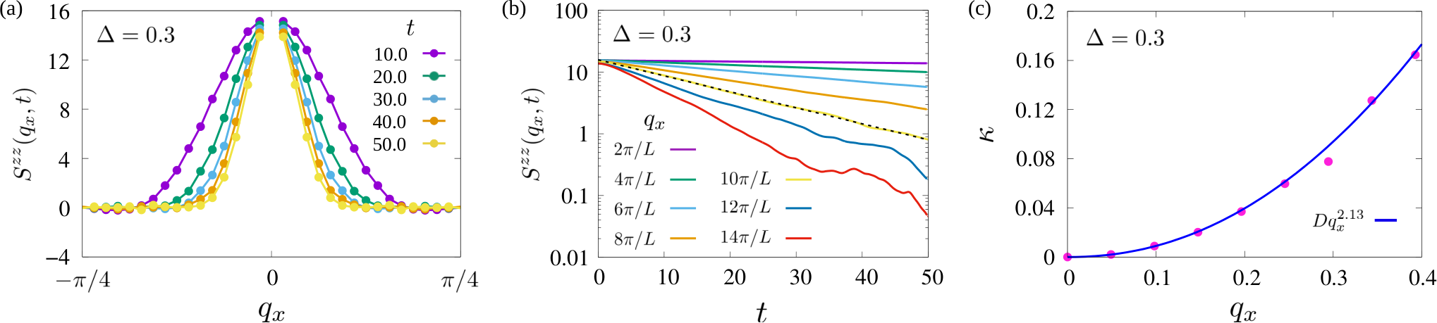
Finally, to probe further the high-temperature diffusive phase and the relation between , which superficially looks like a diffusion constant from dimensional ground, and the actual spin diffusion coefficient , we compute the dynamical structure factor (or its Fourier transform)
| (5) |
For computing the above from spin dynamics simulation, we rewrite above expression as . Here is Fourier transform of -component of spins at time . We obtain from a configuration at time , and average over configurations to obtain in Eq.(5). If the system exhibits normal diffusion, for large wavelength we expect to decay exponentially in time, i.e., where the decay rate . We choose momenta along direction, close to and fit with the exponential form to get for a given . Fig.7(a) shows as a function of for several values of in the easy-plane () case at . The Gaussian form, is evident, implying diffusive behaviour. The exponential decay of as a function of for small momenta is shown in Fig.7(b) for the same parameter values. We extract the diffusion constant for a range of temperatures where could be fitted via with . As we show in Fig.8(b) by plotting , follows the quadratic dependence in the high temperature regime, for both easy-plane and easy-axis cases, where the auto-correlation exponent [Figs.6(b),(c)]. An example of near-quadratic dependence of is shown for and in Fig.7(c). At lower temperatures, we find to deviate from the diffusive form and to exhibit oscillatory behaviour as a function of both and (not shown). The oscillatory behaviour is expected [58] below the transition and even slightly above it, due to spin-waves.

The diffusion constant calculated for both easy-plane and easy-axis anisotropies in the high-temperature diffusive regime () is plotted in Fig.8, and compared with , extracted from Fig.3. In the easy-axis case, both and are independent of temperature at high temperatures () and closely approach their infinite-temperature values, however, . In the easy-plane case, varies substantially with temperature even at high temperature and slowly approaches its infinite-temperature value . This behaviour is unlike that of , which varies little with temperature and coincides with its infinite-temperature value . Moreover, we find for the easy-plane case. Nevertheless, our results suggest that is quite distinct from the actual diffusion constant in general, unlike that in a correlated classical spin-liquid state [15] or in quantum systems like strongly or weakly interacting diffusive metals [7, 39, 43, 44]. For the strongly interacting metals, is related to the energy diffusion constant implying that the chaos or scarambling directly controls the thermal diffusion [7, 39]. To this end, our results raise interesting questions about actual physical process governing in the semiclassical limit of 2d XXZ model. For example, it would be interesting to compute the energy diffusion constant for the spin model in future and see whether it corresponds more closely to , rather than the spin diffusion constant that we calculate here.
5 Conclusion
We have studied here the OTOC, and the dynamical spin correlations in the semiclassical limit of the 2d XXZ model. In particular, we have tuned the anisotropy in the model to study the dynamical properties across KT and 2d Ising transitions via simulation of spin precession dynamics as a function of temperature. Thus we obtain a dynamical phase diagram in terms of chaos and spatio-temporal spin correlations for the classical 2d XXZ model. We have computed temperature dependence of the Lyapunov exponent and butterfly speed, which show crossover across the transitions and no effect of critical slowing down. Only relatively sharp signature of the transitions is exhibited by a non-monotonic temperature dependence of butterfly speed having a minimum at the transition.
Overall, we find chaotic growth and spread, and the dynamical correlations above the transitions at high temperature in the easy-plane and easy-axes cases very similar. However, the dynamical spin-spin correlations are very different at intermediate times in the low-temperature KT and Ising ordered phases, and close to the transitions, although chaos still spreads ballistically in these regimes. This leads us back to the question on the connection of chaos and transport. A simple, albeit heuristic, way [67] to obtain ballistic light-cone for chaos from diffusive transport is to take the separable ansatz for the OTOC and plug in the diffusive form . This leads to a velocity-dependent generalized Lyapunov exponent [34, 14, 36] , and naturally gives rise to the relation . However, we find to be very different from , except for the easy-plane case at infinite temperature. More importantly, the simple ansatz clearly fails in the phases exhibiting anomalous diffusion, like Ising ordered phases in the model. Our observation of the anomalous diffusion over a large range of temperature for easy-axis anisotropy in the semiclassical limit of 2d XXZ model is intriguing and it would be good to get a proper understanding of these phenomena and their possible connections to chaos.
We reveal an early-time pre-exponential regime in the form of a temperature-dependent overall delay in the onset of the light cone. The time scale is presumably connected with chaos time scale and originates from the same many-body interactions that give rise to chaotic growth. This result suggests the possibility of extracting new dynamical regime with a suitable choice of the correlation function. Such a regime may even exist for non-chaotic systems, e.g. integrable or fully quantum ones, where there is no exponential growth inside the light cone [34].
In the absence of any good analytical understanding of many-body chaos in classical systems, our results call for the development of a theoretical framework [68] to compute the classical OTOC along the line of that done for quantum systems, in a suitable large- limit [16], or in some perturbative regime [68, 36], like at low temperatures with weakly interacting spin waves. Such a theory may give rise to new insights into the dynamics of interacting classical systems as well as quantum systems in the semiclassical limit. It would be desirable to obtain hydrodynamic description of the OTOC in such classical spin systems with Hamiltonian dynamics or some related tractable toy models, e.g. with random classical Liouvillian dynamics, along the line of those developed for quantum systems [43, 50, 51, 48, 49].
Acknowledgements
We thank Subhro Bhattacharjee, Samriddhi Sankar Ray, Anupam Kundu, Sumiran Pujari and Sriram Ramaswamy for many useful discussions. We specially thank Anupam Kundu for critical reading of the manuscript and useful feedback. SB acknowledges support from The Infosys Foundation, India and SERB (ECR/2018/001742), DST, India.
Funding information
SB acknowledges support from SERB (ECR/2018/001742), DST, India.
Appendix A Thermodynamic Properties

A.1 Spin stiffness and KT transition
To obtain the Kosterlitz-Thouless (KT) transition temperature for , we calculate the spin stiffness , which measures the rigidity of the spin configuration to small twist or rotation of the spins along some direction. For the KT transition the relevant spin stiffness is obtained by twisting the planar components of the spins. The spin stiffness for the model of Eq.1 in the main text can be obtained as
| (6) |
We calculate via MC simulations and apply the Nelson-Kosterlitz universal jump criterion [63] to obtain , as shown in Fig. 9(a).
A.2 Two dimensional (2d) Ising transition
A.3 Spin-wave dispersion
Easy-plane anisotropy
In this case, the spin-wave dispersion is obtained by expanding the dynamical equations [Eq.2, main text] around the ground state, which corresponds to all spins aligned along a direction (say ) in the -plane. In this case, , and Eq.2 (main text) gets reduced to
Using Fourier transformation , it is straightforward to obtain the spin-wave dispersion for for the square lattice
| (8) |
Hence the spin waves are gapless in the easy-plane case.
Easy-axis anisotropy
In this case, the all the spins can be taken to be aligned along direction, and . Following the same method as the easy-plane case, we obtain the spin-wave dispersion
| (9) |
with a spin-wave gap .


Appendix B Classical OTOC
We show the OTOC for a cut along direction for at two temperatures, and in Fig.10(a),(b). The results are qualitatively similar to the easy-plane anisotropy [Fig.2(a),(b)] in the main text, namely the chaos spreads ballistically, as indicated by the light cones , and the light cones start at a finite time , which increases with decreasing temperature.

We extract the light cones, e.g. in Fig.3(c) (main text), by finding the locus of or , as shown in Fig.11(b) for . The delay time and the butterfly speed are calculated by fitting the light cones in Fig.11(b) with the linear form . The results for and have been shown in the main text in Figs.4(a),(b) and Fig.3(d), respectively.


B.1 Trajectory divergence and decorrelation
In all our calculations and results shown in the main text, we consider the decorrelation function [Eq.(3)] or the classical OTOC, which essentially measures how uncorrelated two spin configurations and are. As discussed earlier, the copy differs from initially only at a single site (), namely . One can also consider the trajectory divergence, which is defined . The decorrelation function and trajectory divergence differ at initially at , i.e.
| (10) |
This initial-time difference eventually relaxes in the intermediate time regime where chaos sets in and we get the same exponential growth and ballistic spread characterized by and , respectively, from both of these quantities.
To compare the decorrelation function and the trajectory divergence, we plot in Fig.12 as a function of for a few , for and . exhibits behaviour very similar to [Fig.2(c),(d)]. By definition, starts from and decreases over an early-time regime, followed by a power-law growth till , before it starts growing exponentially from a value . The exponential growth occurs at a later time for . As shown in Fig. 13(a),(b) for and , both the decorrelation function and trajectory divergence give same values of and .
Appendix C Velocity-dependent Lyapunov exponent
As shown in Fig.5(a),(b), the generalized Lyapunov exponent [Eq.(4)] at different can be collapsed into a single curve as a function of a velocity for over a relatively large range around for both outside () and inside () the light cone. However, this range shrinks progressively with decreasing temperature. Over this range, the velocity-dependent Lyapunov exponent can be fitted well with a ballistic form,
| (11) |
as shown, for example, in Fig.14(a) for easy-plane anisotropy at . The deviation from the scaling for in the inset of Fig.14(a) and in Fig.5 is due to the numerical precision. The extracted values of the exponent are plotted as a function of for in Fig.14(b). Here to obtain we have used a linear approximation to the non-linear fitting form in Eq.(11) for and fitted with as the fitting parameter for fixed values of and obtained from Fig.3. The resulting linear fit and the non-linear function are compared with the data for in Fig.14(a). We find at high temperature, but decreases towards with decreasing temperature . We could not get a reliable goodness of fit at lower temperature since the fitting range shrinks substantially for both and for .
To assess the goodness of the fits we obtain the errorbars [Fig.14(a)] in at each in terms of standard error in the mean (SEM), obtained by dividing trajectories generated with different initial conditions at temperature into multiple groups. Based on these errorbars on and fitting of the data for with the linear approximation to Eq.(11) mentioned above, we obtain the error in , and estimate the goodness of fit using [69]
| (12) |
where is number of data points over the fitting range. A healthy fit is defined as , where is slightly less that 1 [69]. The errors in the estimate of and values are indicated in Fig.14(b) for the easy-plane case . We have not carried out detail error analysis for easy-axis anisotropy , but in this case is shown as a function in Fig.14(c).
To verify the possibility of the broadening of the chaos front around , we have also tried to fit for with [34, 42] with as the fitting parameter. We find , consistent with the absence of broadening [34] and the fact that the is more or less linear for [Figs.5,14(a)], over the range of where the scaling collapse works.
Appendix D Dynamical scaling law for OTOC
One can obtain dynamical scaling laws for OTOC and the butterfly speed across finite-temperature phase transitions with diverging length scale, as in the case of quantum critical point (QCP) [53]. To this end we consider
| (13) |
We can write a scaling form for by applying scaling transformation , where is the dynamical exponent, a universal scaling function, and is the correlation length that diverges for for Ising transition in the easy-axis case and for at the KT transition and KT phase for easy-plane anisotropy. Since, for any and , . Choosing , we obtain
| (14) |
We consider two sets of parameters and such that , . At the scrambling time , , hence the scrambling times for the two sets of parameters are related by . Thus the butterfly velocities [] satisfy . Based on this we can write down the scaling form for
| (15) |
where is a scaling function. For , . On the other hand, for finite and , , implying . These scaling forms are valid only for , since needs to be bounded due to causality.
Appendix E Spin auto-correlation functions


We calculate the spin auto-correlation functions from the spin dynamics simulations starting with thermal initial conditions at different temperatures, as discussed in the main text. We mainly look into the planar correlation and out-of-plane correlation . More specifically, we compute
| (16) |
where , as we have for thermal initial conditions. As shown in Fig.9(a)(inset), in the easy-plane case, below since for strong finite-size effect [64]. In the easy-axis case, below due to spontaneous symmetry breaking [Fig.9(b)(inset)].
In Fig.15(a), we show that decays exponentially with a relaxation time for and . Similar exponential decay is observed for the easy-axis case . However, the relaxation time increases approaching the transition for , whereas it decreases for , as shown in Figs.4(a),(b) in the main text. We show [Fig.15(b)] that exhibits a power-law decay for across the Ising transition. The exponent changes from a diffusive value at high temperature to sub-diffusive values () close to , and finally to super-diffusive values () at low temperature [Fig.6(c)]. To verify whether and have attained a steady power-law behaviour within our finite simulation time (), we obtain a time-dependent exponent () for in the easy-plane case [Fig.16(a)] and across for the easy-axis case [Fig.16(b)]. These suggest that a steady power-law exponent is achieve for except at the lowest temperature studied, whereas the exponent shows perceptible drift towards a larger value for .
References
- [1] A. Kitaev, A simple model of quantum holography (2015).
- [2] S. Sachdev and J. Ye, Gapless spin-fluid ground state in a random quantum Heisenberg magnet, Phys. Rev. Lett. 70, 3339 (1993), 10.1103/PhysRevLett.70.3339.
- [3] J. Maldacena and D. Stanford, Remarks on the Sachdev-Ye-Kitaev model, Phys. Rev. D 94, 106002 (2016), 10.1103/PhysRevD.94.106002.
- [4] A. Kitaev and S. J. Suh, Statistical mechanics of a two-dimensional black hole, Journal of High Energy Physics 2019(5) (2019), 10.1007/jhep05(2019)198.
- [5] P. Castiglione, M. Falcioni, A. Lesne and A. Vulpiani, Chaos and Coarse Graining in Statistical Mechanics, Cambridge University Press, USA, ISBN 0521895936 (2008).
- [6] J. Maldacena, S. H. Shenker and D. Stanford, A bound on chaos, Journal of High Energy Physics 2016(8), 1 (2016), 10.1007/JHEP08(2016)106.
- [7] Y. Gu, X.-L. Qi and D. Stanford, Local criticality, diffusion and chaos in generalized Sachdev-Ye-Kitaev models, JHEP 2017(5), 125 (2017), 10.1007/JHEP05(2017)125.
- [8] J. A. N. Bruin, H. Sakai, R. S. Perry and A. P. Mackenzie, Similarity of Scattering Rates in Metals Showing T-Linear Resistivity, Science 339(6121), 804 (2013), 10.1126/science.1227612, https://science.sciencemag.org/content/339/6121/804.full.pdf.
- [9] S. A. Hartnoll, Theory of universal incoherent metallic transport, Nature Physics 11(1), 54–61 (2014), 10.1038/nphys3174.
- [10] S. Banerjee and E. Altman, Solvable model for a dynamical quantum phase transition from fast to slow scrambling, Phys. Rev. B 95, 134302 (2017), 10.1103/PhysRevB.95.134302.
- [11] A. Haldar, S. Banerjee and V. B. Shenoy, Higher-dimensional Sachdev-Ye-Kitaev non-Fermi liquids at Lifshitz transitions, Phys. Rev. B 97, 241106 (2018), 10.1103/PhysRevB.97.241106.
- [12] J. Kim, X. Cao and E. Altman, Low-rank Sachdev-Ye-Kitaev models, Phys. Rev. B 101, 125112 (2020), 10.1103/PhysRevB.101.125112.
- [13] J. Kim, X. Cao and E. Altman, Scrambling versus relaxation in Fermi and non-Fermi Liquids (2020), 2006.02485.
- [14] A. Das, S. Chakrabarty, A. Dhar, A. Kundu, D. A. Huse, R. Moessner, S. S. Ray and S. Bhattacharjee, Light-cone spreading of perturbations and the butterfly effect in a classical spin chain, Phys. Rev. Lett. 121, 024101 (2018), 10.1103/PhysRevLett.121.024101.
- [15] T. Bilitewski, S. Bhattacharjee and R. Moessner, Temperature dependence of the butterfly effect in a classical many-body system, Phys. Rev. Lett. 121, 250602 (2018), 10.1103/PhysRevLett.121.250602.
- [16] T. Scaffidi and E. Altman, Chaos in a classical limit of the Sachdev-Ye-Kitaev model, Phys. Rev. B 100, 155128 (2019), 10.1103/PhysRevB.100.155128.
- [17] S. D. Murugan, D. Kumar, S. Bhattacharjee and S. S. Ray, Many-body chaos in thermalized fluids, Phys. Rev. Lett. 127, 124501 (2021), 10.1103/PhysRevLett.127.124501.
- [18] A. Schuckert and M. Knap, Many-body chaos near a thermal phase transition, SciPost Phys. 7, 22 (2019), 10.21468/SciPostPhys.7.2.022.
- [19] P. Butera and G. Caravati, Phase transitions and Lyapunov characteristic exponents, Phys. Rev. A 36, 962 (1987), 10.1103/PhysRevA.36.962.
- [20] L. Caiani, L. Casetti, C. Clementi and M. Pettini, Geometry of Dynamics, Lyapunov Exponents, and Phase Transitions, Phys. Rev. Lett. 79, 4361 (1997), 10.1103/PhysRevLett.79.4361.
- [21] V. Constantoudis and N. Theodorakopoulos, Nonlinear dynamics of classical Heisenberg chains, Phys. Rev. E 55, 7612 (1997), 10.1103/PhysRevE.55.7612.
- [22] C. Dellago and H. Posch, Lyapunov instability in the extended XY-model: Equilibrium and nonequilibrium molecular dynamics simulations, Physica A: Statistical Mechanics and its Applications 237(1), 95 (1997), https://doi.org/10.1016/S0378-4371(96)00423-2.
- [23] L. Caiani, L. Casetti, C. Clementi, G. Pettini, M. Pettini and R. Gatto, Geometry of dynamics and phase transitions in classical lattice theories, Phys. Rev. E 57, 3886 (1998), 10.1103/PhysRevE.57.3886.
- [24] L. Caiani, L. Casetti and M. Pettini, Hamiltonian dynamics of the two-dimensional lattice model, Journal of Physics A: Mathematical and General 31(15), 3357 (1998), 10.1088/0305-4470/31/15/004.
- [25] X. Leoncini, A. D. Verga and S. Ruffo, Hamiltonian dynamics and the phase transition of the XY model, Physical Review E 57(6), 6377–6389 (1998), 10.1103/physreve.57.6377.
- [26] T. Kawabe and S. Ohta, Scaling behavior of Lyapunov exponents in Abelian-Higgs theories, Phys. Rev. D 61, 105013 (2000), 10.1103/PhysRevD.61.105013.
- [27] A. S. de Wijn, B. Hess and B. V. Fine, Largest Lyapunov Exponents for Lattices of Interacting Classical Spins, Phys. Rev. Lett. 109, 034101 (2012), 10.1103/PhysRevLett.109.034101.
- [28] A. S. de Wijn, B. Hess and B. V. Fine, Lyapunov instabilities in lattices of interacting classical spins at infinite temperature, Journal of Physics A: Mathematical and Theoretical 46(25), 254012 (2013), 10.1088/1751-8113/46/25/254012.
- [29] A. S. de Wijn, B. Hess and B. V. Fine, Chaotic properties of spin lattices near second-order phase transitions, Physical Review E 92(6) (2015), 10.1103/physreve.92.062929.
- [30] M. Das and J. R. Green, Critical fluctuations and slowing down of chaos, Nature Communications 10(1) (2019), 10.1038/s41467-019-10040-3.
- [31] R. J. Deissler, One-dimensional strings, random fluctuations, and complex chaotic structures, Physics Letters A 100(9), 451 (1984), https://doi.org/10.1016/0375-9601(84)90823-5.
- [32] K. Kaneko, Lyapunov analysis and information flow in coupled map lattices, Physica D: Nonlinear Phenomena 23(1), 436 (1986), https://doi.org/10.1016/0167-2789(86)90149-1.
- [33] R. J. Deissler and K. Kaneko, Velocity-dependent Lyapunov exponents as a measure of chaos for open-flow systems, Physics Letters A 119(8), 397 (1987), https://doi.org/10.1016/0375-9601(87)90581-0.
- [34] V. Khemani, D. A. Huse and A. Nahum, Velocity-dependent Lyapunov exponents in many-body quantum, semiclassical, and classical chaos, Phys. Rev. B 98, 144304 (2018), 10.1103/PhysRevB.98.144304.
- [35] P. M. Chaikin and T. C. Lubensky, Principles of Condensed Matter Physics, Cambridge University Press, 10.1017/CBO9780511813467 (1995).
- [36] T. Bilitewski, S. Bhattacharjee and R. Moessner, Classical many-body chaos with and without quasiparticles, Phys. Rev. B 103, 174302 (2021), 10.1103/PhysRevB.103.174302.
- [37] B. V. Fine, T. A. Elsayed, C. M. Kropf and A. S. de Wijn, Absence of exponential sensitivity to small perturbations in nonintegrable systems of spins 1/2, Phys. Rev. E 89, 012923 (2014), 10.1103/PhysRevE.89.012923.
- [38] P. C. Hohenberg and B. I. Halperin, Theory of dynamic critical phenomena, Rev. Mod. Phys. 49, 435 (1977), 10.1103/RevModPhys.49.435.
- [39] R. A. Davison, W. Fu, A. Georges, Y. Gu, K. Jensen and S. Sachdev, Thermoelectric transport in disordered metals without quasiparticles: The Sachdev-Ye-Kitaev models and holography, Phys. Rev. B 95, 155131 (2017), 10.1103/PhysRevB.95.155131.
- [40] D. Stanford, Many-body chaos at weak coupling, Journal of High Energy Physics 2016(10) (2016), 10.1007/jhep10(2016)009.
- [41] D. Chowdhury and B. Swingle, Onset of many-body chaos in the model, Phys. Rev. D 96, 065005 (2017), 10.1103/PhysRevD.96.065005.
- [42] S. Sahu and B. Swingle, Information scrambling at finite temperature in local quantum systems, Phys. Rev. B 102, 184303 (2020), 10.1103/PhysRevB.102.184303.
- [43] I. L. Aleiner, L. Faoro and L. B. Ioffe, Microscopic model of quantum butterfly effect: Out-of-time-order correlators and traveling combustion waves, Annals of Physics 375, 378 (2016), https://doi.org/10.1016/j.aop.2016.09.006.
- [44] A. A. Patel, D. Chowdhury, S. Sachdev and B. Swingle, Quantum butterfly effect in weakly interacting diffusive metals, Phys. Rev. X 7, 031047 (2017), 10.1103/PhysRevX.7.031047.
- [45] D. J. Luitz and Y. Bar Lev, Information propagation in isolated quantum systems, Phys. Rev. B 96, 020406 (2017), 10.1103/PhysRevB.96.020406.
- [46] B. Dóra and R. Moessner, Out-of-time-ordered density correlators in luttinger liquids, Phys. Rev. Lett. 119, 026802 (2017), 10.1103/PhysRevLett.119.026802.
- [47] A. Keselman, L. Nie and E. Berg, Scrambling and lyapunov exponent in spatially extended systems, Phys. Rev. B 103, L121111 (2021), 10.1103/PhysRevB.103.L121111.
- [48] V. Khemani, A. Vishwanath and D. A. Huse, Operator spreading and the emergence of dissipative hydrodynamics under unitary evolution with conservation laws, Phys. Rev. X 8, 031057 (2018), 10.1103/PhysRevX.8.031057.
- [49] C. W. von Keyserlingk, T. Rakovszky, F. Pollmann and S. L. Sondhi, Operator hydrodynamics, otocs, and entanglement growth in systems without conservation laws, Phys. Rev. X 8, 021013 (2018), 10.1103/PhysRevX.8.021013.
- [50] A. Nahum, S. Vijay and J. Haah, Operator spreading in random unitary circuits, Phys. Rev. X 8, 021014 (2018), 10.1103/PhysRevX.8.021014.
- [51] T. Rakovszky, F. Pollmann and C. W. von Keyserlingk, Diffusive hydrodynamics of out-of-time-ordered correlators with charge conservation, Phys. Rev. X 8, 031058 (2018), 10.1103/PhysRevX.8.031058.
- [52] A. Nahum, J. Ruhman, S. Vijay and J. Haah, Quantum entanglement growth under random unitary dynamics, Phys. Rev. X 7, 031016 (2017), 10.1103/PhysRevX.7.031016.
- [53] B.-B. Wei, G. Sun and M.-J. Hwang, Dynamical scaling laws of out-of-time-ordered correlators, Phys. Rev. B 100, 195107 (2019), 10.1103/PhysRevB.100.195107.
- [54] G. Aarts and J. Smit, Classical approximation for time dependent quantum field theory: Diagrammatic analysis for hot scalar fields, Nucl. Phys. B 511, 451 (1998), 10.1016/S0550-3213(97)00723-2, hep-ph/9707342.
- [55] S. Sachdev, Quantum Phase Transitions, Cambridge University Press, second edn. (2011).
- [56] E. Nakano, V. Skokov and B. Friman, Transport coefficients of scalar field theories close to the critical point, Phys. Rev. D 85, 096007 (2012), 10.1103/PhysRevD.85.096007.
- [57] J. Berges, S. Schlichting and D. Sexty, Dynamic critical phenomena from spectral functions on the lattice, Nuclear Physics B 832(1-2), 228–240 (2010), 10.1016/j.nuclphysb.2010.02.007.
- [58] H. G. Evertz and D. P. Landau, Critical dynamics in the two-dimensional classical XY model: A spin-dynamics study, Phys. Rev. B 54, 12302 (1996), 10.1103/PhysRevB.54.12302.
- [59] D. P. Landau and M. Krech, REVIEW ARTICLE: Spin dynamics simulations of classical ferro- and antiferromagnetic model systems: comparison with theory and experiment, Journal of Physics Condensed Matter 11(18), R179 (1999), 10.1088/0953-8984/11/18/201.
- [60] D. R. Nelson and D. S. Fisher, Dynamics of classical spins in one and two dimensions, Phys. Rev. B 16, 4945 (1977), 10.1103/PhysRevB.16.4945.
- [61] J. M. Kosterlitz and D. J. Thouless, Ordering, metastability and phase transitions in two-dimensional systems, Journal of Physics C: Solid State Physics 6(7), 1181 (1973), 10.1088/0022-3719/6/7/010.
- [62] J. M. Kosterlitz, The critical properties of the two-dimensional xy model, Journal of Physics C: Solid State Physics 7(6), 1046 (1974), 10.1088/0022-3719/7/6/005.
- [63] D. R. Nelson and J. M. Kosterlitz, Universal jump in the superfluid density of two-dimensional superfluids, Phys. Rev. Lett. 39, 1201 (1977), 10.1103/PhysRevLett.39.1201.
- [64] S. T. Bramwell and P. C. W. Holdsworth, Magnetization: A characteristic of the Kosterlitz-Thouless-Berezinskii transition, Phys. Rev. B 49, 8811 (1994), 10.1103/PhysRevB.49.8811.
- [65] D. Bagchi, Spin diffusion in the one-dimensional classical Heisenberg model, Phys. Rev. B 87, 075133 (2013), 10.1103/PhysRevB.87.075133.
- [66] A. Das, K. Damle, A. Dhar, D. A. Huse, M. Kulkarni, C. B. Mendl and H. Spohn, Nonlinear fluctuating hydrodynamics for the classical xxz spin chain, Journal of Statistical Physics 180(1-6), 238–262 (2019), 10.1007/s10955-019-02397-y.
- [67] B. Swingle and D. Chowdhury, Slow scrambling in disordered quantum systems, Phys. Rev. B 95, 060201 (2017), 10.1103/PhysRevB.95.060201.
- [68] S. Banerjee, Unpublished (2020).
- [69] P. Young, Everything you wanted to know about Data Analysis and Fitting but were afraid to ask, arXiv e-prints arXiv:1210.3781 (2012), 1210.3781.