Transient processes in a gas / plate structure in the case of light gas loading
Abstract
Problems of pulse excitation in an acoustic waveguide with a flexible wall and in an acoustic half-space with a flexible wall are studied. In both cases the flexible wall is described by a thin plate equation. The solutions are written as double Fourier integrals. The integral for the waveguide is computed explicitly, and the integral for the half-space is estimated asymptotically. A special attention is paid to the pulse, which is a harmonic wave of a finite duration associated with the coincidence point of the dispersion diagrams of the acoustic medium and the plate. The method of estimating of the double Fourier integral is applied to the problem of excitation of waves in a system composed of an ice plate, water substrate, and the air.
1 Introduction
The paper is motivated by a simple experiment. A thin ( cm) layer of ice on a lake or a pond should be hit with a stick or stone. Let a listener be located on the surface of the lake quite far from the place where the ice is hit (about 200 m). The listener shall hear a long quasi-monochromatic “whistle” instead of a kick. The sound is surprising and unexpected. The current paper describes such a signal mathematically.
The qualitative explanation of the effect is rather simple. The impact on the ice generates a wide spectrum of bending waves, propagating along the ice plate. The bending oscillation of the ice is then a source of the sound that is recorded in the air.
It is important that the bending waves possess dispersion. The higher is the frequency, the greater is the phase velocity. At some circular frequency , that is called the coincidence frequency, the phase velocity of the wave coincides with the air sound velocity . At this frequency, the acoustic wave propagating in a sliding way along the ice has the same phase velocity as the bending wave, and the energy transfer from the ice plate to the sound wave is the most effective. One can show by measurements that the pulse related to the coincidence point has a narrow–band spectrum centered at the coincidence frequency.
As usual, the dispersion of the bending waves in the ice leads to emerging of the concept of the group velocity, i. e. of the velocity of narrow-band pulse propagation. For a bending plate without loading, the relation between the wavenumber and the temporal frequency is , thus the group velocity is two times bigger than the phase velocity:
A detailed study (see below) shows that the air and water loading does not change this situation qualitatively. The group velocity of the bending waves at the coincidence frequency is equal to if the water substrate is ignored, and can be roughly estimated as if the water is taken into account. The waves in the air going horizontally are dispersionless, thus the group velocity for them is equal to the phase velocity : .
Immediately after the impact, the components of the spectrum at the coincidence frequency start to radiate sound into the air. As the group velocity of bending waves is about twice as much as the air waves, the wave packet bearing the radiating harmonics propagates to the observation point, permanently leaving behind the sound radiated earlier in the air (see Fig. 1, a).
The sound signal appears at the observation point only when the wave packet of bending waves comes to this point (see Fig. 1, b). After that, the sound radiated earlier by the distant points comes. The sound signal vanishes only when the sound from the start point comes.
The pulse duration is equal to the difference between arrival time of the head of the bending waves packet at the coincidence frequency and the arrival time of the sound wave of the impact itself :

The experimental setup described above is still rather complicated for analytical modeling. We simplify it by making the geometry two–dimensional and by eliminating the water layer underlying the ice, i. e. only the plate (ice) and the gas (air) are considered. Moreover, we assume that the air loading is light, i. e. that the air wave does not affect the process in the plate.
Two physical situations are considered in the paper. The first one is a thin waveguide with a rigid wall and a flexible wall. The second physical situation is a flexible plate loaded by gas half-plane on one side. We are mostly interested in the second problem, however the first one can be solved analytically, and thus it can be used to check the statements made for the second one.
For each formulation, the wave excitation problem can be solved formally by the Fourier transform. As the result, the wave pulse becomes described as a 2D Fourier integral. The aim of this paper is to obtain an asymptotic estimation of this integral.
The assumption of light gas loading simplifies the consideration a lot. The physical system becomes split into two subsystem: the heavy one (the plate), and the light one (the gas). The denominator of the integrand of the Fourier integral is expressed as a product of two functions, each of which can be treated as a dispersion function for an isolated subsystem. The zero sets of the dispersion functions are branches of the dispersion diagram of the system. The branches of the dispersion diagram are crossing. It is known that if the interaction between the subsystems is not negligible, there exists a so-called avoiding crossing of the branches instead of a crossing. An estimation of a 2D Fourier integral with singularities having an avoiding crossing seems to be a more complicated task.
Beside two model problems, we formulate a considerably more complicated problem corresponding to the experiment with the ice layer. However, we demonstrate that the methods developed in the paper can be applied to this problem as well. Moreover, we show that the experimental signal displays some properties that follow from our analysis.
The interaction of waves in an elastic plate and a surrounding liquid or gas is a well-studied topic. This is an interesting analytical problem having important practical applications. Rather than writing a comprehensive review of the subject, we mention here only the papers important for the research below.
A 3D problem of a point source time–harmonic excitation of a plate loaded by a liquid was formulated and solved by using the Fourier–Bessel transformation in [1]. The energy carried by sonic waves was computed. Besides, the formal solution of the same problem in terms of the Fourier integral can be found in [2, 3]. A basic analysis of the integral from [1] was performed in [4] with the help of the saddle point method. Particularly, an asymptotic estimation of the Fourier integral in the far field zone for the frequencies below the coincidence frequency was found.
“Free waves” corresponding to the poles of the Fourier integral are discussed in [5, 6, 7]. These poles form a complicated structure if the loading of the plate cannot be considered as light: they obey an equation of degree 5 even for the simplest plate equation.
A thick plate (elastic layer) immersed in the fluid was studied in [6, 7, 8]. Plates governed by sophisticated equations of motion were considered in [9, 10, 11, 12]. A Timoshenko–Mindlin plate loaded by a layered medium was studied in [13]. All such problems can be addressed by the techniques described in [14].
In [15, 16] the dispersion equation was approximated by a rational function. The acoustical radiated field was calculated under this approximation.
A systematic study of heavy/light loading of plates and membranes was performed in [5, 17, 18, 19, 20]. The importance of the parameter describing the lightness of the loading was stressed (this parameter tends to zero in our study below). The regimes were classified. The results were summarised in the 1988 Rayleigh medal lecture by Crighton [21]. An asymptotic expression for a leaky wave in the case of a lightly loaded plate at frequencies above the coincidence was presented in [5]. A lightly loaded membrane excited by a concentrated force was studied in [18]. This paper should be mentioned especially because the author built a “map of asymptotics” covering the whole range of the parameters. In [19] some asymptotic results for a heavily loaded plate were obtained. In [22] an intermediate regime of loading was studied, when the fluid loading was heavy enough to affect the surface waves, but the inertia of the plate still could be considered as negligible.
Most of the papers (and almost all above) dealt with a time-harmonic wave excitation. Only a few considered a transient regime. The reason for this is the absence of well established methods for asymptotic estimation of 2D Fourier integrals. Note that we develop such methods, but only for the simplest case of light loading.
A formal solution of the transient problem in an integral form was obtained in [10, 22]. Some works devoted to transient processes in fluid–loaded elastic plates are [23, 24]. The paper most close to the current study was [25], where a series of contour deformations was performed. The 2D problem was studied there. An expression for a first arrival pulse was obtained. In [26, 27, 28] transient processes were studied numerically.
The pulse related to the coincidence point of the dispersion diagram was considered in [29]. The energy of the pulse was estimated.
The current paper is organized as follows. In Section 2, the problems of wave excitation in a waveguide with a flexible wall and in a half-space with a flexible wall are formulated and solved by the Fourier transformation. Also we formulate a 3D problem for a realistic 3D configuration of an ice layer loaded by air a and by a water substrate. In Section 3, a solution for the waveguide with an flexible wall is computed rigorously by a residue integration. In Section 4, the integral for the half-space with a flexible wall is estimated. According to the “main statement” of asymptotic estimation formulated in this section, only the crossings of branches of the dispersion diagram and the saddle points on the dispersion diagrams should be taken into account. As a result, a “library” of asymptotics related to different fragments of the dispersion diagram is developed. In Section 5, we briefly comment on the 3D problem with water loading. Namely, we the influence of the water substrate, show how our methods can be applied to the Fourier–Bessel integral, comment on the system with absorption, and propose an interpretation of the experimental results. In Appendix, the standard integrals used for the asymptotic study are described.
2 Formulation of the problems and integral representations of the field
2.1 Problem 1. Gas / plate waveguide
The geometry of the problem is as follows. A gas layer occupies the domain in the -plane (see Fig. 2, left). An elastic plate made of an isotropic material is the layer . Assume that is small and that the bending waves in the plate are described by the linear thin plate theory [30].
The plate is stress-free at the surface , the contact conditions are fulfilled at the surface , and the surface is acoustically hard (impenetrable). The source is applied to the plate at the point . The time profile of the source is the Dirac’s delta-function.

Describe waves in the gas by an acoustic potential . The acoustic potential is linked with the pressure and the particle velocity components by the relations [2]
| (1) |
where is the (constant) gas density. The governing equation in the gas is the wave equation
| (2) |
where is the (constant) wave velocity in the gas.
Let be the vertical displacement of the plate. The equation of motion of the plate can be written as [30]
| (3) |
Here is the density of the plate,
| (4) |
is the flexural stiffness of the plate ( is the Young’s modulus of the elastic material, and is the Poisson’s ratio), is the amplitude of excitation.
The second term in the left-hand side of Eq. (3) is responsible for the gas loading, and the right-hand side corresponds to the point source excitation.
The boundary conditions for the air layer are
| (5) |
| (6) |
Our aim is to find the pressure in the gas near the plate, i. e. the function . The solution should be causal, i. e. the field components and should be equal to zero for .
To solve the problem formulated as Eqs (2-6), introduce the Fourier transform with respect to and the Laplace transform with respect to :
| (7) |
Note that the variable of the Laplace transform is chosen to be , so the resulting notations are “Fourier-like”. The inverse of this transform is
| (8) |
where is an arbitrary positive parameter.
Using these transformations, one can write down the acoustic pressure near the plate in the form of a double integral
| (9) |
where
| (10) |
The value of the square root Eq. (10) is selected in such a way that it has a positive imaginary part on the whole integration plane. This choice provides existence of only decaying waves in the air. Also, it leads to continuous on the integration plane.
Let us make two simplifications of Eq. (9). First, let be small, i. e. let the gas loading of the plate be light (some discussion can be found in [5, 19, 22]). The second term in the denominator can be neglected comparatively to the first one on the whole integration plane:
| (11) |
where
| (12) |
The second simplification for Eq. (9) is to assume that the air waveguide is narrow, i. e. to take . The assumption yields , , and
| (13) |
Physically, this assumption means that only the piston mode is allowed to propagate in the acoustic part of the waveguide.
The resulting representation Eq. (13) is one of the simplest integrals possessing a pulse related to the coincidence point in its asymptotics.
The denominator of Eq. (13) has two factors that are related to the plate and to the air piston mode. Introduce the real dispersion diagrams
| (14) |
Introduce also the complex dispersion diagrams , as the sets
| (15) |
Indeed, the real dispersion diagrams are subsets of corresponding complex dispersion diagrams. Analytical continuation of a dispersion diagram proved itself to be a useful tool in the analysis of transient processes in waveguides [31, 32, 33, 34].
The points of correspond to the waveguide modes in the plate, namely to the functions
which are solutions of the equation of motion for an unloaded plate without sources. The similar statement is valid for the set and the gas layer with Neumann walls. Indeed, is the dispersion diagram for piston modes in such a layer.
Let be a crossing point of the diagrams and :
| (16) |
All intersection of the dispersion diagrams and are as follows:
| (17) |
Indeed, all these points are real.
The real dispersion diagrams and and the crossing point are sketched in Fig. 3.

2.2 Problem 2. 1D bending plate loaded by a 2D half-space
Let the gas occupy the half-plane , and the plate (the same as in the previous subsection) is attached to the half-plane along the line (see Fig. 2, right). The wave process in the gas is described by the wave equation Eq. (2), and the plate is described by equation Eq. (3). Condition Eq. (5) is omitted, and Eq. (6) remains valid. It is not necessary to introduce a radiation condition, since for a causal solution it should be valid automatically.
Let us look for the acoustic pressure in the gas near the plate, i. e. at . The solution of the problem can be obtained using the same method as above:
| (18) |
The air loading is assumed to be light, thus representation Eq. (18) can be simplified as follows:
| (19) |
The zeros of the denominator of Eq. (19) are described by the same functions and .
2.3 Problem 3. Ice, air, and water in 3D space
The previous two problems are relatively simple, and they will be studied in details below. In this subsection we formulate mathematically the problem that motivated our research, namely the 3D problem of excitation of an ice plate loaded by a water substrate below and by a light air above. The excitation is a pulse of force applied to the ice plate at some point. The receiver is located in the air near the ice at the distance from the source point.
This problem is considerably more complicated than the model ones, so we are not planning to study it in details. However, we are going to describe the term related to the coincidence point using the method developed on the basis of the model problems. In this case, the coincidence point occurs as a crossing point of the dispersion diagram of the air and the dispersion diagram of the bending waves in the ice on the water substrate.
The geometry of the problem is shown in Fig. 4. The -axis is directed normally to the plane of the figure and is not shown. The water occupies the domain , all the rest is similar to Problem 2.

The acoustic field in the air is described by the wave equation
| (20) |
( is the wave velocity in the air). The acoustic field in the water is described by the wave equation
| (21) |
Here is the wave velocity in the water, and is the acoustic potential in the water. The acoustic pressure in the water is
| (22) |
where is the density of the water. The pressure in the air is defined by the first equation of Eq. (1).
We assume that the ice bears only the bending waves described by the equation
| (23) |
which is a modification of Eq. (3). is the flexural stiffness of the ice (see Eq. (4)), and is the density of the ice.
The continuity condition for the air / ice interface is Eq. (6), and for the water / ice interface is
| (24) |
We have to find the air pressure .
The system of equations formulated above can be easily solved by applying the Laplace transform with respect to and the Fourier transform with respect to and . The result can be written in the form of the Fourier–Bessel integral:
| (25) |
where
| (26) |
and is the Bessel function.
Introduce the dispersion equation for bending waves in ice loaded by water:
| (27) |
In our consideration we assume that the air loading is light, and water loading is considerable. Thus, at least locally, one can neglect the last term in the denominator and obtain a simplified representation for the pressure:
| (28) |
One can see that there are two factors in the denominator of the integrand. One corresponds to waves in the air, while the other corresponds to waves in the ice plate loaded by the water. The coincidence point is the common zero of both functions:
| (29) |
Our aim is to describe the processes described by the integral Eq. (28) estimated near this point.
3 Computation of the integral Eq. (13) (Problem 1)
The integral Eq. (13) can be easily computed analytically.
For any with , the integrand is a regular function on the real axis of and near this real axis. For simplicity, slightly deform the integration contour in the -plane such that the deformed contour coincides with the real axis almost everywhere, and bypasses above the points . Denote this contour by . This choice of the contour is arbitrary, and the result remains the same if the contour passes below the points .
First, take the internal integral in the -domain using the residue method. The contour of integration should be closed in the lower half-plane, since the factor decays there for . For a fixed , there are four poles , , and all of them fall within the closed contour. The result is a
| (30) |
where
| (31) |
| (32) |
The integrals can be taken using the residue method:
| (33) |
| (34) |
The integrals can be expressed through the Fresnel’s integrals:
| (35) |
| (36) |
where for real is the Fourier integral defined by Eq. (A.36) in Appendix A3. Representations Eq. (35) and Eq. (36) follow from the non-trivial formula Eq. (A.35). The bar sign denotes the complex conjugation here and below.
Let us analyze the solution. Introduce the “formal velocity”
| (37) |
Consider the asymptotics , . Introduce also the value
| (38) |
and the function
| (39) |
Use the asymptotics Eq. (A.37) and Eq. (A.38) for for . As the result, if the asymptotics is as follows:
| (40) |
where C.C. denotes the complex conjugated terms, is the pulse mainly attributed to the plate wave:
| (41) |
is the pulse mainly attributed to the piston wave in the gas waveguide:
| (42) |
and is the pulse related to the coincidence point of the dispersion diagram:
| (43) |
Note that due to the problem symmetry.
In the intermediate zone the argument of function is of order of 1. No asymptotics of can be used in this zone, so one should use the function itself. For a fixed large , the width of the intermediate zone in the variable is as follows:
| (44) |
Thus, this width grows as . It is important that this width grows, but slower than linearly.
The term is a purely monochromatic pulse with a smooth front at and an abrupt front at . The values and are, thus, the boundaries of the domain occupied by the term in the plane. These values emerged in our research quite naturally in the process of getting the explicit solution. We should note that and are the values of the group velocity of the branches of the dispersion diagram at the crossing point . Below we discuss this feature in details and demonstrate that the pulse related to the coincidence point of the dispersion diagram always have fronts linked to the group velocities of the interacting modes.
Note also that the field is continuous at since the sum is continuous there.
4 Estimation of Eq. (19) (Problem 2)
Unfortunately, the integral Eq. (19) cannot be taken explicitly. So our next aim is to develop a technique of evaluation of such an integral in a general situation. As above, we fix the value and take to build the asymptotic procedure. The idea of the technique is quite standard: the surface of integration should be deformed in such a way that the integrand is exponentially small everywhere except neighborhoods of several “special points”. These points are the saddle points on the real dispersion diagrams and the crossing points of the dispersion diagrams. The integrals over the neighborhoods of the “special points” can be taken approximately (asymptotically). Some typical integrals of this sort are listed in the Appendix.
4.1 Overview of the surface deformation procedure. The “main statement” and its proof
At each point of the branches of the dispersion diagrams one can define the group velocity
| (45) |
The group velocities at the points of the real branches are real.
The saddle points on the real branches of the dispersion diagrams are the points at which
| (46) |
Let us find the position of the saddle point on , for which . The group velocity is then
| (47) |
The saddle point has coordinates with
| (48) |
The main statement of the estimation procedure is as follows:
For almost all values of , the terms of the field not decaying exponentially as are produced by the fragments of the integration surface that are located in neighborhoods of either the saddle points on the real branches, or the crossing points of the real branches of the dispersion diagrams.
The idea of the proof is as follows. Consider the integral Eq. (19) as an integral of an analytic differential 2-form over some surface (smooth manifold) [35]:
| (49) |
where
| (50) |
and is an oriented manifold with , . According to the 2D Cauchy’s theorem, one can deform continuously the manifold , and the value of the integral should remain the same if the manifold does not cross the singular sets of the integrand form during the course of deformation.
To estimate the integral, one has to find a deformation of into a new manifold , such that the integrand is exponentially small almost everywhere, i. e. such that
| (51) |
The neighborhoods on where one cannot fulfill the inequality Eq. (51) are used to build the estimation of the wave field components.
We consider only small deformations of . Since is large, a small deformation is enough to fulfill Eq. (51).
Let the deformed integration manifold be parametrized by real parameters as follows:
| (52) |
where , are some smooth real functions. The deformation process can be described using a parameter . For this, introduce a family of integration surfaces:
| (53) |
One can see that
Let be a real point belonging to the dispersion diagram . Consider a small complex neighborhood of . Let us describe the eligible deformations of in this neighborhood, i. e. the deformations in which the manifold of integration does not cross .
Let the group velocity of the corresponding branch of the dispersion diagram at be equal to . A point in this neighborhood belongs to the complex branch of the dispersion diagram only if
| (54) |
(indeed, this is not a sufficient condition). This follows from the fact that
| (55) |
Let the deformation of in the neighborhood of be chosen in such a way that the functions , are locally constant. Let be . Consider the conditions Eq. (54) and Eq. (51) graphically. It is a difficult task to display a 2D manifold in a 4D space, so we choose to plot projections of the integration manifolds onto the coordinate plane . A fragment of the initial manifold is projected onto a single point in this plane. Corresponding fragment of the deformed manifold is shown also as a single point . The deformation process is the motion along the segment connecting these points (see Fig. 5, left).

The inequality Eq. (51) is fulfilled is the resulting point is located above the line (with a margin of the height equal to ). The line is shown by the bold solid line in the figure.
The manifold can hit the singularity only if the segment crosses the line on which Eq. (54) is valid. This line is shown dotted in the figure. This means that if the segment does not cross the dotted line, then the deformation is eligible.
An inverse statement is much more subtle, but it also can be proven: If the segment crosses the dotted line in the diagram, then crosses the singularity set at some points, and the deformation is not eligible.
One can see that the eligible deformation in the case looks like it is shown in Fig. 5, left. The point belongs to the first quadrant of the coordinate plane. This deformation will be referred to as a deformation of the “” type.
If then the eligible deformation is as shown in Fig. 5, center. The point now belongs to the third quadrant of the coordinate plane. This deformation will be referred to as the deformation of the “” type.
For the “special points” (the saddle points or the crossing points of the dispersion diagrams) we need a deformation that does not obey Eq. (51), but still does not cross the singularities. Such a deformation is called “0” type, and is shown in Fig. 5, right.
Let grow continuously from to . The point then goes far into the first quadrant. One can see that the “” type deformation cannot be transformed continuously into the “” type deformation. Therefore, between the domains of “” type deformation and “” type deformation there should be a zone with “” type deformation. This is a very important conclusion, since the domains with “” or “” type deformation do not produce non-vanishing field components, while the domains with the “0” type can produce such components.
Finally, if , only a “” type deformation is eligible, and it looks as shown in Fig. 6.

The deformation should be made carefully only near the real branches of the dispersion diagram. We assume that an eligible smooth deformation can be easily found in the rest of the -plane, since there are no obstacles for deformation at such places. This is why, below we indicate the type of the deformation only for the neighborhoods of the real branches of the dispersion diagram.
4.2 Integration surface deformation for the integral Eq. (19)
In this subsection we analyze the deformation of the integration surface for Eq. (19) in terms of the types of the deformation introduced above. Note that the singular sets of Eq. (13) and Eq. (19) are the same, so the conclusions obtained here can be applied to Eq. (13) as well, and the exact value of Eq. (13) can be examined on its compliance with our asymtotic theory.
The integrand of Eq. (19) has the real branches of the dispersion diagram named and . The group velocity takes all values from to on . For each , there exist two saddle points on . On , the group velocity takes values only.
There are five crossing points Eq. (17) of the dispersion diagrams and . The group velocity on is equal to at the non-zero crossing points.
Let be . Fig. 7, left, shows how the deformation type should be chosen in this case. The saddle points on are marked by symbol “s”. The “”, “”, and “0” types of surface deformation are marked by corresponding signs.


Consider the saddle point with positive and . The group velocity on is bigger than to the right of the saddle point and is smaller than to the left of the saddle point. Thus, near , one should choose the “” type of the surface deformation to the right, and “” type of the deformation to the left. Since the deformation should be continuous, one should choose the “0” type of the deformation in the neighborhood of the saddle point. Thus, the saddle points on produce non-vanishing components of the wave field.
Indeed, there should be some continuous transition between “0” type and the “”/“” types.
All other branches are labeled with “+” type deformation. In particular, for each of five crossing points, all branches crossing at them are of the “” type. Therefore, the vicinities of the crossing points can be shifted according to the “” type, and the crossing points do not produce non-vanishing field components.
Let be . Corresponding deformation diagram is shown in Fig. 7, right. The neighborhood of the crossing point changes its status comparatively to Fig. 7, left. The branch should be deformed according to the “” type, while should be deformed according to the “” type. Since the deformation is continuous, the neighborhood of the crossing point should be of the “” type. Therefore, the the crossing point produces a non-vanishing field component. Besides, the saddle point on (also deformed according to the “” type) produces another field component.
Consider the case . The diagram is shown in Fig. 8. The neighborhood of the crossing point can now be deformed according to the “” type, and thus it does not produce non-vanishing field components. The crossing point should be deformed according to the “” type, since one branch crossing at this point is deformed according to the “” type, while all other branches are deformed according to the “” type. Besides, there are saddle points on that also produce non-vanishing components.

When , the saddle point is close to the crossing point of the branches of the dispersion diagram. This case produces an intermediate asymptotics and it should be considered in a special way. The diagram is shown in Fig. 9, left. One can see that the zone of “0” type deformation covers both the crossing point and the saddle point


The most sophisticated case is . In this case, the whole neighborhood of the branch is tangential to the line (see Fig. 9, right), and thus it cannot be analyzed locally.
Let us summarize this diagram consideration. The saddle point on produces a non-vanishing component for all , the crossing point produces a non-vanishing component only for , and the crossing point produces a non-vanishing component only for .
One can see that corresponding wave components are analogous to , , and from Eq. (40) for the integral Eq. (13). The last component is the pulse related to the coincidence point of the dispersion diagram. Thus, the qualitative analysis based on deformation of the integration surface is in agreement with the exact solution.
Remark. The case requires a special consideration, since the “0”-deformation zone is elongated in the vertical direction. However, this case is not considered in this paper, since it requires more complicated standard integrals.
4.3 Local estimations of the integral Eq. (19)
According to the analysis of the surface integral deformation, if is not close to , , or , one can expect to obtain an asymptotic estimation of Eq. (19) in the form
| (56) |
where is the complex conjugation operator. The terms in the right are the following wave components:
-
is produced by the saddle point on with positive and ,
-
is produced by the saddle point on with negative and ,
-
is produced by the crossing point of dispersion diagrams at ,
-
is produced by the crossing point of dispersion diagrams at ,
-
is produced by the crossing point of dispersion diagrams at .
The terms and are non-zero for all , the term is non-zero for , the terms and are non-zero only for .
Note that definition of in Eq. (56) is slightly different from that of Eq. (40) (factor 2 is omitted for convenience).
In the zone the estimation of the field can be found in the form
| (57) |
where is the term produced by the crossing point and the neighboring saddle point.
In the zone the estimation of the field is as follows:
| (58) |
where is the saddle-point term introduced above, and is the term produced by the elongated zone located along the branch in Fig. 9, right.
The width of the zone can be estimated using a standard reasoning based on the concept of the “domain of influence” [36]. Namely, belongs to the intermediate zone if the phase difference between the crossing point and the saddle point is of order of 1. This happens if
| (59) |
Using Eq. (48), one can get the estimation , where is defined by Eq. (38), so Eq. (44) is valid.
To have a consistent set of asymptitotic expansions, the term should have asymptotics
| (60) |
| (61) |
Similarly, one can estimate the width of the intermediate zone . The condition is as follows: the phase difference between the points and should be of order of 1:
| (62) |
resulting in
| (63) |
For consistency, function should have the following asymptotics:
| (64) |
| (65) |
The scheme of all asymptotics is shown in Fig. 10. This scheme shows the zones of validity of asymptotics in the -domain for a large fixed . The scheme does not cover small values of (i. e. large values of ). The matching rules Eqs (60,61,64,65) guarantee the consistency of the scheme.

The terms of Eq. (56) have different physical nature. The term is a dispersive bending wave in the plate accompanied by some sound pressure in the surrounding air. The term is the sound radiated into the air by the supersonic part of the bending pulse. The term can be interpreted as the wave traveling in air and radiated mainly by the initial impact point.
Below we obtain approximations for the terms of the asymptotics.
Estimation of
Approximate the algebraic factors of the integrand of Eq. (19) near as follows:
Evaluation of corresponding integral is shown in Appendix A2. The parameter is equal to 1. The result of application of formula Eq. (A.21) is
| (66) |
Estimation of
Approximate the algebraic function in the integrand near the origin as follows:
| (67) |
This approximation can be used if is not very small comparatively to . The integral
can be estimated as the integral Eq. (A.1) from Appendix A. The parameters for the integral are , , , , . Formula Eq. (A.16) can be applied. The result is
| (68) |
Estimation of
Estimate the algebraic function in the integrand near the point as follows:
| (69) |
To estimate the integral, one can use the method described in Appendix A1. This is the integral of the type Eq. (A.1) with , , , , , . Formula Eq. (A.15) can be used. The result is
| (70) |
Estimation of
Assume that . Use the first approximation Eq. (69). Apply the procedure of estimation described in Appendix A3. The standard integral is Eq. (A.23) with , , , , .
The estimation of the integral is given by Eq. (A.43). The result is
| (71) |
4.4 Non-local estimation of Eq. (19) for
Consider the case . Our aim is to build an estimation of the integral over a long spot marked by “0” sign and located along the branch in Fig. 9, right. In other words, the aim is to compute from Eq. (58).
Let be
| (72) |
Change the order of integration in Eq. (19) and take the integral with respect to for a fixed . For this, shift the integration contour into the upper half-plane since the factor decays there. Note that there are two poles and a branch point in the upper half-plane of . The poles are and , while the branch point is . After the deformation, the contour will look as shown in Fig. 11.

The integral can be written as
| (73) |
where the first two terms are the residue integrals:
| (74) |
| (75) |
The branch point integral can be estimated for large :
| (76) |
The contours for the first two integrals can be deformed as it is shown in Fig. 12 and estimated for large . The result of the estimation for each integral is a sum of a saddle point term and of the branch cut term. We are interested only in the branch cut term, since the saddle point terms are equal to and for . Denote the branch cut terms of and by and , respectively. Their estimations are

| (77) |
Estimate the integral Eq. (76). If the contour of integration can be closed in the upper half-plane, and . If the contour should be shifted into the lower half-plane. The deformed contour is shown in Fig. 13. It consists of two polar terms and the branch term. Let the polar terms for the poles and be and , respectively. Let the branch cut integral be denoted by :
| (78) |

A detailed computation yields
| (79) |
| (80) |
The last expression can be rewritten as
| (81) |
where
| (82) |
Some properties of function are displayed in Appendix A4.
Finally,
| (83) |
From Eq. (77) if follows that
This means that there is no intermediate zone before the front , i. e. the representation remains valid for all even for small . Indeed, this guarantees Eq. (64).
The width of the intermediate zone is . This agrees with Eq. (63).
4.5 Taking into account absorption in the plate
For the motivating air / ice / water problem it is natural to expect that the ice plate possesses some absorption. Here our aim to analyze the influence of this absorption on the asymptotic estimation of the integral. For simplicity, we use the model integral Eq. (19) for this study.
The absorption of bending waves is modeled in the simplest way: the bending stiffness of the plate is assumed to have a small negative imaginary part:
| (84) |
Thus, the Young modulus of the plate has a small negative imaginary part, and all other physical parameters are real. Such a model is rather elementary, and it can describe correctly only the neighborhood of the coincidence point . This model may be invalid for the other crossing points and for the low- and high-frequency components, but our aim is to demonstrate here the applicability of our method on the simplest possible example.
The presence of the negative imaginary part of leads to a small positive imaginary part of :
| (85) |
According to the dispersion diagram
| (86) |
the value for positive real has a positive imaginary part, and for positive real has a negative imaginary part. This corresponds to decaying waves of slightly different types.
The complex dispersion diagram still can be defined for Eq. (86), while the real dispersion diagram is empty. Thus, our asymptotic analysis should be slightly modified.
The dispersion diagram possesses the following fundamental energetic property near : if and is real, then has a negative imaginary part. Obviously, this property guarantees that energy decays in the system. To see that the property should be valid, one can consider a resonator made of the plate, having the length of , and bearing the periodicity condition at the ends. The value is the eigenvalue of this resonator, and the negative imaginary part of corresponds to decay. As it follows from this property, does not intersect the initial integration manifold .
Instead of the real dispersion diagram , one can introduce the approximately real dispersion diagram, which is the set of points having small values of and .
Let us find the intersection point as a crossing of and , i. e. a solution of the equations Eq. (86) and . Indeed, the solution is Eq. (16). However, now and both have positive imaginary parts.
One can introduce the saddle points on . Namely, since is an analytic set, the (complex) group velocity is defined by Eq. (45) at almost all points of . The saddle points are the points at which the group velocity is equal to the formal velocity , i. e. where Eq. (46) is valid. Note that the group velocity at a saddle point is real, but the point itself can be complex.
The main statement of the asymptotic estimation procedure formulated in Subsection 4.1 should be reformulated as follows: For almost all values of , the leading terms of the asymptotics of the double Fourier integral are produced by the fragments of the integration surface that are located in neighborhoods of either the saddle points on the approximately real branches or the crossing points of the approximately real branches.
Note that now the leading terms of the asymptotics can be exponentially decaying as due to the energy absorption.
The sketch of the proof of this statement is direct modification of that from Subsection 4.1. The only new part that should be added is the deformation of in the case of
In this case, in the linear approximation, the intersection of with the plane , is a point rather than a line. Thus, any contour not passing through this point will be an eligible deformation.
The procedure of estimation of the integrals near the crossing points and the saddle points remains the same. Indeed, the formulae for terms , , and also remain the same, but one should take into account that is complex.
The term represented as Eq. (70) has an important feature for complex . Since has a positive imaginary part, this term is exponentially growing as grows. This does not contradict to our consideration, since the field should be decaying (and is decaying) as with constant . The exponential growth of can be explained physically. For some fixed , the smaller is , the bigger distance the signal traveled in the plate before being radiated into the gas. Since the plate has losses, the smaller correspond to the smaller signal.
5 Comments to Problem 3
5.1 The preliminary analysis
In this section we are analyzing Problem 3 and its solution Eq. (28). First, let us illustrate the influence of water on the bending waves in ice. Take the thickness of ice equal to cm, and the physical parameters as
We assume that ice is lossless.
Fig. 14 shows the dispersion diagrams for with defined as Eq. (27). It is labeled as the curve “with water” in the graph. For a comparison, we plot also the set (the curve labeled as “without water”), and labeled as . The coincidence point Eq. (29) is indicated in the figure. One can see that the water affects the dispersion diagram of bending waves considerably, however qualitatively the diagrams are similar.
The coincidence frequencies and of bending waves have been computed for the range cm. The result is presented in Fig. 15.


The system Eq. (29) can be reduced to an algebraic equation. Let it be solved (say, numerically) for a given , and let the values and be known. Then, one compute the derivatives
| (87) |
| (88) |
The group velocity of the bending waves can be found according to the theorem of the implicit function:
| (89) |
Denote this value by .
A direct computation shows that the group velocity of the bending waves in the ice loaded by water is about for the range 1…10 cm, i. e. is slightly higher than . A good estimation is for the experiment.
5.2 Estimation of Eq. (28) near the intersection point
The integral Eq. (28) doesn’t have a form of a 2D Fourier integral, so it should be transformed to make our method applicable to it. Still, we assume that the analysis based on the locality remains valid. We are focusing here only on the terms related to the coincidence points .
Assume that
| (90) |
In this case the Bessel function can be represented as
| (91) |
Introduce the formal velocity by . Let be . Consider a neighborhood of the point . Formula Eq. (92) shows that there are two terms in this integral. The first term corresponds to the deformation diagram shown in Fig. 7, right. Thus, this term provides a non-decaying asymptotics. For the second term of Eq. (92), one can select the “” type deformation shown in Fig. 16 for both crossing branches. This means that the second term does not lead to a non-decaying asymptotics.

Thus, the task is reduced to estimation of the integrals
| (93) |
where are the fragments of the integration surface in the neighborhoods of .
The resulting integrals have the form similar to those have been studied. They are double Fourier integrals whose denominators contain a crossing of a quadratic branch set and a polar set. Thus, these integrals can be estimated by using the technique described above, providing the terms similar to , , and of Eq. (56) and Eq. (57).
The non-local term similar to requires some special consideration , which is beyond the scope of the current paper. Still, we believe that its structure is qualitatively similar to what has been found above.
5.3 Experimental results and their interpretation
Let us demonstrate the experimental results obtained by one of the authors. The acoustic signals have been recorded for the parameters cm and m. Note that the thickness of ice is known very approximately, and we should admit that it could be varying over the lake surface due to natural reasons.
The shape of a typical signal is shown in Fig. 17. The zero mark of the time was not set properly, so the exact starting time of the signal is not known. We assume that, mainly, the signal caused by the coincidence point is visible (this is in Eq. (56)). The duration of the pulse is about 0.25 s, and this agrees very well with the rough estimation .

The spectrogram of the signal is shown in Fig. 18, left. The spectrogram is obtained with short-time Fourier transform with a reasonable Gaussian window function. The vertical axis shows the frequency .
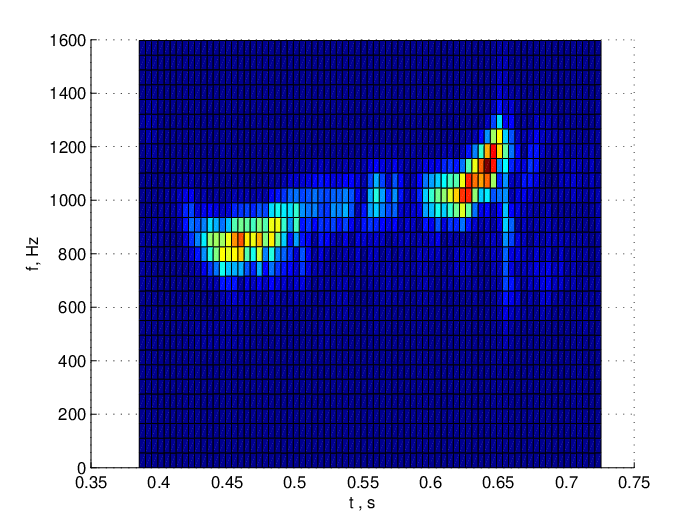

Our interpretation of the spectrogram is shown in Fig. 18, right. The main component is . It is almost monochromatic. The frequency agrees with the thickness of ice. The reason of frequency elevation at the end of the signal is unclear, we can assume that the thickness of ice decreased closer to the shore. The variations of the amplitude of this pulse are probably described by a sort of speckle pattern.
At the start of the pulse one can see the fragment of the signal . This signal is strongly dispersive: the parts with higher frequencies go faster. That’s why the frequency decays with time. An estimation of the slope of the spectrogram is
| (94) |
This estimation works reasonably well for the observed signal.
The zone of mixing of and should be described by the term of Eq. (56). For illustration, we plot a model spectrogram of the function Eq. (71) in Fig. 19. The structure of the spectrogram is easily explained by the asymptotics Eq. (A.40), Eq. (A.41). The inclined line corresponds to the first term of Eq. (A.40) and to the term Eq. (A.41). The straight line corresponds to the second term of Eq. (A.40).
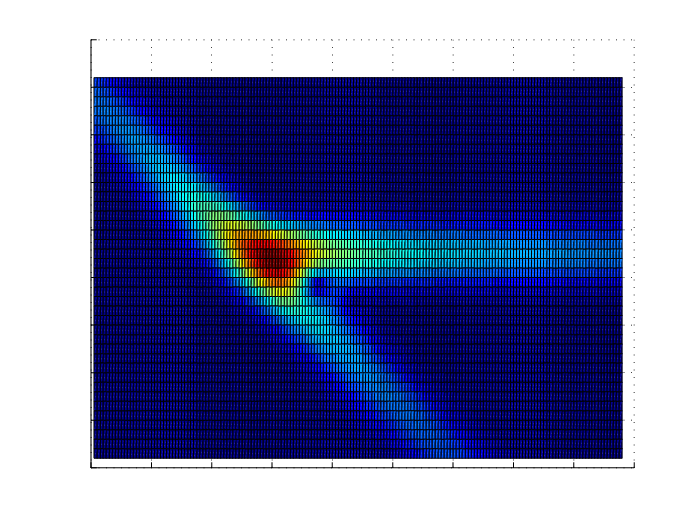
The back front of the pulse is visible as a vertical line in the spectrogram. This corresponds to a fast process in time. Our estimation of the width of the pulse is . The frequency band of such a pulse is about kHz, and this agrees with the spectrogram.
The main problem for the interpretation is the dependence of the amplitude of the term vs. time. The asymptotic formula Eq. (A.15), which remains valid for the term due to the coincidence point, yields the amplitude dependence which a decaying function for . However, Fig. 17 shows that the back part of the pulse has the amplitude bigger than the front part. One possible explanation is the presence of decay in the ice. As we claimed above, the factor is exponentially growing in time if the ice is lossy. Another reason for the complicated behavior of amplitude of vs time may be a refraction of sound wave near the surface of ice.
To provide a detailed description of the experiment, one should take into account that the altitude of the microphone was about m height, not zero. The signal (the sound wave accompanying the bending wave in the ice) strongly depends on the altitude of the microphone. The part with corresponds to supersonic radiation of sound wave, so this component should be clearly visible in the recording. The part of with corresponds to the subsonic radiation, and this wave should be exponentially decaying in the air. The characteristic length is about the wavelegth, i. e. about 30 cm. However, although the subject seems to be interesting and practically important, the asymptotic estimation of the Fourier integral with falls beyond the scope of the current paper.
6 Conclusions
The paper can be summarized as follows. The integrals Eq. (13) and Eq. (19) are analyzed. Both integrals describe non-stationary wave processes in two-component systems with a high density contrast between the subsystems. The expressions Eq. (13) and Eq. (19) are 2D Fourier integrals. The denominators of the integrands have zero sets that are crossing.
The paper contains an exact computation of Eq. (13) and an asymptotic estimation of Eq. (19). In both cases we find a monochromatic pulse existing for . The frequency and the wavenumber of this pulse are equal to those of the point of phase synchronism of the subsystems (the coincidence point).
A general scheme of estimation of a 2D Fourier integral is presented. The procedure of estimation is based on the fact (the “main statement”) that the field components are produced by saddle points on the branches of the dispersion diagrams and by crossing points of the branches of the dispersion diagrams. A set of standard integrals related to such points are given in Appendix.
The “main statement” is formulated for a very particular case: the branches of the dispersion diagram are graphs of slowly varying functions. Here “slowly varying” means that the size of a typical zone of variation of and is much bigger than the size of the domain of influence (DOI in terms of [36]) for a saddle point integral. Note that in a general case, the dispersion diagram contains avoiding crossing where the function changes in a small zone. Our “main statement” does not work in the general case, and it should be replaced by a more sophisticated theorem.
Although the methods developed in this paper are applicable to double Fourier integrals, we demonstrate how they can be applied to a more realistic 3D problem of sound generation by the ice layer loaded by the water substrate. Such a problem describes the experimental setting that is a motivation of the paper. The solution of the problem is described by a Fourier intergal in time and a Fourier–Bessel integral in space. We demonstrate that some methods of estimation still can be applied to this integral.
The spectrogram of the signal is interpreted in terms of the asymptotic analysis. The main features of the experimental signal are explained correctly by our analysis, namely the frequency of the main signal, its duration, the structure of the front and the back of the pulse.
The work can be continued in four directions. First, one can consider avoiding–crossings instead of crossings of the dispersion diagrams. As it is known, this is a more realistic situation emerging when the contrast between subsystems is not very high. Second, one can study the field at the observation point not close to the horizontal surface. This leads to appearance of the factor , which makes the estimation procedure different. Third, one can introduce and study more of the standard integrals. For example, finding the asymptotics of Eq. (19) for requires a standard integral with two square root singularities, two polar singularity and a double zero. Fourth, the deformations of the integration manifold described here can be used to develop efficient methods of numerical computation of double Fourier integrals.
Acknowledgements
AVS thanks Prof. C.J. Chapman for fruitful discussions of the waveguide subjects during the INI programme WHT: “Bringing pure and applied analysis together via the Wiener–Hopf technique, its generalizations and applications”. The WHT programme was supported by EPSRC (grant no. EP/R014604/1). The visit of AVS to the INI program and his work on non-local asymptotical expansion has been partly supported by the grant from the Simon’s foundation.
The study of standard integrals has been funded by RFBR, project number 19-29-06048.
References
- [1] L. M. Brekhovskikh and I. E. Tamm. On the forced vibrations of an infinite plate in contact with water. Zhournal of Technical Physics (in Russian), 16:879–888, 1946.
- [2] P.M. Morse and K.U. Ingard. Theoretical acoustics. New York: McGraw-Hill, 1968.
- [3] M.C. Junger and D. Feit. Sound, structures, and their interaction, volume 225. MIT press Cambridge, MA, 1986.
- [4] L.Ya. Gutin. Sound radiation from an infinite plate excited by a normal point force. Sov. Phys. Acoust, 10(4):369–371, 1965.
- [5] D.G. Crighton. The free and forced waves on a fluid-loaded elastic plate. Journal of Sound and Vibration, 63(2):225–235, mar 1979.
- [6] S.I. Rokhlin, D.E. Chimenti, and A.H. Nayfeh. On the topology of the complex wave spectrum in a fluid-coupled elastic layer. The Journal of the Acoustical Society of America, 85(3):1074–1080, mar 1989.
- [7] A. Freedman. Anomalies of the a0leaky lamb mode of a fluid-loaded, elastic plate. Journal of Sound and Vibration, 183(4):719–737, jun 1995.
- [8] S.V. Sorokin. Analysis of time harmonic wave propagation in an elastic layer under heavy fluid loading. Journal of Sound and Vibration, 305(4-5):689–702, sep 2007.
- [9] D. Feit. Pressure radiated by a point-excited elastic plate. The Journal of the Acoustical Society of America, 40(6):1489–1494, dec 1966.
- [10] A.D. Stuart. Acoustic radiation from submerged plates. I. influence of leaky wave poles. The Journal of the Acoustical Society of America, 59(5):1160, 1976.
- [11] A.D. Stuart. Acoustic radiation from submerged plates. II. radiated power and damping. The Journal of the Acoustical Society of America, 59(5):1170, 1976.
- [12] J.D. Smith. Symmetric wave corrections to the line driven, fluid loaded, thin elastic plate. Journal of Sound and Vibration, 305(4-5):827–842, sep 2007.
- [13] V. M. Kurtepov. Sound field of a point source in the presence of a thin infinite plate in the medium (discrete spectrum). Soviet Physics - Acoustics, 15:484–490, 1970.
- [14] L. M. Brekhovskih and R. T. Beyer. Waves in Layered Media. Academic Press, 1980.
- [15] D.T. DiPerna and D. Feit. An approximate analytic solution for the radiation from a line-driven fluid-loaded plate. The Journal of the Acoustical Society of America, 110(6):3018–3024, dec 2001.
- [16] D.T. DiPerna and D. Feit. An approximate green’s function for a locally excited fluid-loaded thin elastic plate. The Journal of the Acoustical Society of America, 114(1):194–199, jul 2003.
- [17] D.G. Crighton. Approximations to the admittances and free wavenumbers of fluid-loaded panels. Journal of Sound and Vibration, 68(1):15–33, jan 1980.
- [18] D.G. Crighton. The green function of an infinite, fluid loaded membrane. Journal of Sound and Vibration, 86(3):411–433, feb 1983.
- [19] D.G. Crighton. The modes, resonances and forced response of elastic structures under heavy fluid loading. Philosophical Transactions of the Royal Society of London. Series A, Mathematical and Physical Sciences, 312(1521):295–341, oct 1984.
- [20] D. G. Crighton, Ann P. Dowling, J. E. Ffowcs Williams, M. A. Heckl, and F. A. Leppington. Modern Methods in Analytical Acoustics. Springer London, 1992.
- [21] D.G. Crighton. The 1988 rayleigh medal lecture: Fluid loading—the interaction between sound and vibration. Journal of Sound and Vibration, 133(1):1–27, aug 1989.
- [22] C.J. Chapman and S.V. Sorokin. The forced vibration of an elastic plate under significant fluid loading. Journal of Sound and Vibration, 281(3-5):719–741, mar 2005.
- [23] E.B. Magrab and W.T. Reader. Farfield radiation from an infinite elastic plate excited by a transient point loading. The Journal of the Acoustical Society of America, 44(6):1623–1627, dec 1968.
- [24] A.D. Stuart. Acoustic radiation from a point excited inifinite elastic plate. PhD thesis, The Pensilvania State University, 1972.
- [25] Mackertich S.S. and S.I. Hayek. Acoustic radiation from an impulsively excited elastic plate. The Journal of the Acoustical Society of America, 69(4):1021–1028, apr 1981.
- [26] J.H. James. Sound radiation from infinite thin plate. Technical Report ARE TM(UHA) 87508, Admiralty research establishment, 1987.
- [27] R. Scherrer, L. Maxit, J.-L. Guyader, C. Audoly, and M. Bertinier. Analysis of the sound radiated by a heavy fluid loaded structure excited by an impulsive force. Internoise 2013, 09 2013.
- [28] A. Langlet, M. William-Louis, G. Girault, and O. Pennetier. Transient response of a plate–liquid system under an aerial detonation : Simulations and experiments. Computers & Structures, 133:18–29, mar 2014.
- [29] A.V. Akol’zin and M.A. Mironov. Energy flows in media caused by a normally excited plate near the frequency of coincidence (in russian). Trudy nauchnoi scholy prof S. A. Rubaka, 2:90, 2001.
- [30] L.D. Landau. Theory of Elasticity, volume 7. Elsevier LTD, Oxford, 2004.
- [31] Philip Wayne Randles. Modal Representations for the High-Frequency Response of Elastic Plates. PhD thesis, 1969.
- [32] P.W. Randles and J. Mlklowitz. Modal representations for the high-frequency response of elastic plates. International Journal of Solids and Structures, 7(8):1031–1055, aug 1971.
- [33] A. V. Shanin. Precursor wave in a layered waveguide. The Journal of the Acoustical Society of America, 141(1):346–356, jan 2017.
- [34] A.V. Shanin, K.S. Knyazeva, and A.I. Korolkov. Riemann surface of dispersion diagram of a multilayer acoustical waveguide. Wave Motion, 83:148–172, dec 2018.
- [35] B.V. Shabat. Introduction to complex analysis. American Mathematical Society, 1992.
- [36] V.A. Borovikov. Uniform stationary phase method. Institution of Electrical Engineers, London, 1994.
Appendix A Standard local integrals
A.1 Crossing of two singular sets
Consider the integral
| (A.1) |
with
| (A.2) |
where , , , are some real values. One can see that the integrand of Eq. (A.1) has two singular sets (lines):
The lines are crossing at the point . The values and are group velocities of the “dispersion diagrams” at the crossing point. Let be . We do not assume that and are positive.
Let us find the asymptotics of as and .
Real parameters determine the type of singularities. We are particularly interested in the cases (a polar set), or (a branching with integrable singularity). Assume for definiteness that the function is positive real if the argument is positive real, and that this function is continuous on the integration surface.
Introduce the variables
| (A.3) |
The integral can be rewritten as
| (A.4) |
Note that the integration contour in the plane , , passes below the real axis if and above the real axis if . Using this fact, close the contours of integration in appropriate half-planes and obtain that
| (A.5) |
If , then
| (A.6) |
| (A.7) |
where if and if . Contours and are shown in Fig. A.1.

Compute . If is not a positive integer then
| (A.8) |
| (A.9) |
is the Gamma-function.
If is a positive integer than
| (A.10) |
| (A.11) |
In particular, for positive
| (A.12) |
| (A.13) |
Let be , . Then
| (A.14) |
Let be , , . Then
| (A.15) |
Finally, let be , . Then
| (A.16) |
A.2 A saddle point on a singular set
Consider the integral
| (A.17) |
where
| (A.18) |
Parameters , , , are real. Parameter is small. One can see that the point is a saddle point of the integral on the dispersion diagram . Indeed,
Introduce the coordinates
| (A.19) |
After a deformation of the integration surface, obtain
| (A.20) |
The integral can be taken:
| (A.21) |
where
| (A.22) |
A.3 A saddle point near a crossing point of singular sets
Consider the integral
| (A.23) |
| (A.24) |
| (A.25) |
Let be . Assume that , i. e. the saddle point belongs to the branch .
Introduce the variables
| (A.26) |
| (A.27) |
Solve the equations
with respect to the variables and . To get convenient formulae, assume that the term is small, and the equation can be solved iteratively. After the second iteration obtain
| (A.28) |
| (A.29) |
Using these approximations, write the exponential factor of in the form
| (A.30) |
Since , the factor in the second term is small, and the size of the integration domain in is much bigger than the size in . Thus, one can replace by :
| (A.31) |
The integral can be written approximately as
| (A.32) |
where
| (A.33) |
| (A.34) |
where the contour of integration of integration is shown in Fig. A.2.

Function is rather complicated. We consider two cases. For
| (A.35) |
where is the Fresnel integral
| (A.36) |
The well-known formula Eq. (A.35) can be proven by differentiation of Eq. (A.34) with respect to .
If the function
| (A.39) |
can be expressed through the functions of the parabolic cylinder [36]. However, it is simple to tabulate directly by using the definition Eq. (A.34). The real and imaginary part of the function computed numerically are plotted in Fig. A.3.

A.4 A special function for the non-local estimation

Function has the following asymptotics for :
| (A.45) |
We also note that
| (A.46) |