”This work has been submitted to the IEEE for possible publication. Copyright may be transferred without notice, after which this version may no longer be accessible.”
Observing the Invisible: Live Cache Inspection
for
High-Performance Embedded Systems
Abstract
The vast majority of high-performance embedded systems implement multi-level CPU cache hierarchies. But the exact behavior of these CPU caches has historically been opaque to system designers. Absent expensive hardware debuggers, an understanding of cache makeup remains tenuous at best. This enduring opacity further obscures the complex interplay among applications and OS-level components, particularly as they compete for the allocation of cache resources. Notwithstanding the relegation of cache comprehension to proxies such as static cache analysis, performance counter-based profiling, and cache hierarchy simulations, the underpinnings of cache structure and evolution continue to elude software-centric solutions.
In this paper, we explore a novel method of studying cache contents and their evolution via snapshotting. Our method complements extant approaches for cache profiling to better formulate, validate, and refine hypotheses on the behavior of modern caches. We leverage cache introspection interfaces provided by vendors to perform live cache inspections without the need for external hardware. We present CacheFlow, a proof-of-concept Linux kernel module which snapshots cache contents on an NVIDIA Tegra TX1 SoC (system on chip).
Index Terms:
cache, cache snapshotting, ramindex, cacheflow, cache debuggingI Introduction
The burgeoning demand for high-performance embedded systems among a diverse range of applications such as telemetry, embedded machine vision, and vector processing has outstripped the capabilities of traditional micro-controllers. For manufacturers, this has engendered a discernible shift to system-on-chip modules (SoCs). Coupled with their extensibility and improved mean time between failures, SoCs offer improved reliability and functionality. To bridge the gap between increasingly faster CPU speeds and comparatively slower main memory technologies (e.g. DRAM) most SoCs feature cache-based architectures. Indeed, caches allow modern embedded CPUs to meet the performance requirements of emerging data-intensive workload. At the same time, the strong need for predictability in embedded applications has rendered analyses of caches and their contents vital for system design, validation, and certification.
Unfortunately, this interest runs counter to the general desire to abstract complexity. Cache mechanisms and policies are ensconced entirely in hardware, to eliminate software interference and encourage portability. Consequently, software-based techniques used to study caches suffer from several shortcomings, which we detail in Section V-E.
In contrast, we propose CacheFlow: a technique that can be implemented in software and in existing high-performance SoCs to extract and analyze the contents of cache memories. CacheFlow can be deployed in a live system without the need for an external hardware debugger. By periodically sampling the cache state, we show that we can reconstruct the behavior of multiple applications in the system; observe the impact of scheduling policies; and study how multi-core contention affects the composition of cached content.
Importantly, our technique is not meant to replace other cache analysis approaches. Rather, it seeks to supplement them with insights on the exact behavior of applications and system components that were not previously possible. While in this work we specifically focus on last-level (shared) cache analysis, the same technique can be used to profile private cache levels, TLBs, and the internal states of coherence controllers. In summary, we make the following contributions:
- 1.
This is the first paper to describe in detail an interface, namely RAMINDEX, available on modern embedded CPUs that can be used to inspect the content of CPU caches. Despite its usefulness, the interface has received little to no attention in the research community thus far;
- 2.
We present a technique called CacheFlow to perform cache content analysis via event-driven snapshotting;
- 3.
We demonstrate that the technique can be implemented on modern hardware by leveraging the RAMINDEX interface and propose a proof-of-concept open-source Linux implementation11 1 Our implementation can be found at: https://github.com/weirdindiankid/cacheflow
- 4.
We describe how to correlate information retrieved via cache snapshotting to user-level and kernel software components deployed on the system under analysis;
- 5.
We evaluate some of the insights provided by the proposed technique using real and synthetic benchmarks.
The rest of this paper is organized as follows: in Section II, we document related research that inspired and informed this paper. In Sections III and IV, we provide a bird’s-eye view of the concepts necessary to understand the mechanics of CacheFlow. In Sections V and VI, we detail the fundamentals of CacheFlow and its implementation. Section VII outlines the experiments we performed and documents their results. We also examine the implications of those results. Section VIII concludes the paper with an outlook on future research.
II Related Work
Caches have a significant impact on the temporal behavior of embedded applications. But their design—oriented toward programming transparency and average-case optimization—makes performance impact analysis difficult. A plethora of techniques have approached cache analysis from multiple angles. We hereby provide a brief overview of the research in this space.
Static Cache Analysis derives bounds on the access time of memory operations when caches are present [1, 2, 3]. Works in this domain study the set of possible cache states in the control-flow graph (CFG) of applications. Abstract interpretation is widely employed for static cache analysis, as first proposed in [4] and [5]. For static analysis to be carried out, a precise model of the cache behavior is required. Techniques that consider Least-Recently Used (LRU), Pseudo-LRU, and FIFO replacement policies [6, 7, 3, 8, 9] have been studied.
Symbolic Execution is a software technique for feasible path exploration and WCET analysis [10, 11] of a program subject to variable input vectors. It proffers a middle ground between simulation and static analysis. An interpreter follows the program; if the execution path depends on an unknown, a new symbolic executor is forked. Each symbolic executor stands for many actual program runs whose actual values satisfy the path condition.
As systems grow more complex, Cache Simulation tools are essential to study new designs and evaluate existing ones. Simulation of the entire processor — including cores, cache hierarchy, and on-chip interconnect — was proposed in [12, 13, 14, 15]. Simulators that only focus on the cache hierarchy were studied in [16, 17, 18]. Depending on the component under analysis, simulations abound. In the (i) execution-driven approach, the program to be traced runs locally on the host platform; in the (ii) emulation-driven approach, the target program runs on an emulated platform and environment created by the host; finally, in the (iii) trace-driven approach, a trace file generated by the target application is fed into to the simulator. An excellent survey reviewing 28 CPU cache simulators was published by Brais et. al [19]. The most popular is perhaps Cachegrind that belongs to the Valgrind Suite [20].
Statistic Profiling is performed by leveraging performance monitoring units (PMUs) integrated in modern processors. PMUs can monitor a multitude of hardware events that occur as applications execute on the platform. Unlike the aforementioned strategies, sampling the PMU provides information on the real behavior of the hardware platform. As such, a number of works have used statistic profiling to study memory-related performance issues [21, 22, 23]. High level libraries such as PAPI [24, 25], Likwid [26] and numap [27] provide a set of APIs to ease the use of PMUs.
Despite the seminal results achieved in the last decade in the cache analysis and profiling techniques described thus far, a few important limitations are worth noting. Techniques that rely on cache models — i.e. static analysis, symbolic execution, simulation — work under the assumption that the employed models accurately represent the true behavior of the hardware. Unfortunately, complex modern hardware often deviates from textbook models in unpredictable ways. Access to event counters subsequently only reveals partial information on the actual state of the cache hierarchy.
The technique proposed in this paper is meant to complement the analysis and profiling strategies reviewed thus far. It does so by allowing system designers to snapshot the actual content of CPU caches. This, in turn, enables a new set of strategies to extract/validate hardware models, or to conduct application and system-level analysis on the utilization of cache resources. Unlike works that proposed cache snapshotting by means of hardware modifications [28, 29, 30] our technique can be entirely implemented in software and leverages hardware support that already exists in a broad line of high-performance embedded CPUs.
III Background
In this section, we introduce a few fundamental concepts required to understand CacheFlow’s inner workings. First, we review the structure and functioning of multi-level set-associative caches. Next, we briefly explore the organization of virtual memory in the target class of SoCs.
III-A Multi-Level Caches
Modern high-performance embedded processors implement multiple levels of caching. The first level (L1) is the closest to the CPU and its contents are usually private to the local processor. Cache misses in L1 trigger a look-up in the next cache level (L2), which can be still private, shared among a subset (cluster) of cores, or globally shared by all the cores. Additional levels (L3, L4, etc.) may also be present.
The last act before a look-up in the main memory is to query the Last-Level Cache (LLC). Without loss of generality, and to be more in line with our implementation, we consider the typical cache layout of ARM-based processors. That is, we assume private L1 caches and a globally shared L2, which is also the LLC.
Set-associativity: Caching at any level typically follows a set-associative scheme. A set-associative cache with associativity , features ways, where each way has an identical structure. A cache with total size is thus structured in ways of size each. Caches store multiple blocks of consecutive bytes in cache lines (a.k.a. cache blocks). We use to indicate the number of bytes in each cache line. Typical line sizes are 32 or 64 bytes. denotes the number of lines in a way or sets in a cache.
When the CPU accesses a cacheable memory location, the memory address determines how the cache look-up (or allocation) is performed. In the case of a cache miss, the least-significant bits of the address encode the specific byte inside the cache line and are called offset bits. For instance, in systems with bytes, the offset bits are [5:0]. The second group of bits in the memory address encodes the specific cache set in which the memory content can be cached. Since we have possible sets, the next bits after the offset bits select one of the possible sets and are called index bits. Finally, the remaining bits, called tag bits, are stored alongside cached content to detect cache hits after look-up.
Virtual and Physical Caches: Addresses used for cache look-ups can be physical or virtual. In the vast majority of embedded multi-core systems, tag bits are physical address bits signifying a physically-tagged cache. In shared caches (e.g. L2), index bits are also derived from physical addresses. For this reason, they are said to be physically-indexed, physically-tagged (PIPT) caches [31, 32, 33, 34, 35].
III-B Memory Management & Representation
Virtual Memory Modern computing architectures rely on software and hardware support to map virtual addresses used by processes to physical addresses represented in the hardware. Giving processes distinct views of the system’s memory obviates problems stemming from fragmentation or limited physical memory. The operating system manages the translation between virtual and physical addresses through a construct known as the page table. When a process tries to reference a virtual address, the operating system first checks for that address’ presence in the referencing process’ address space. If present, the system then checks for the page’s presence in memory via its page table entry (PTE). From there, the address is either resolved to a physical address, or the page is brought into main memory and then resolved.
Virtual Memory Areas: When a process terminates in Linux, the kernel is tasked with freeing the process’ memory mappings. Older versions of Linux accomplished this by iterating through a chain of reverse pointers to page tables that referenced each physical frame. The mounting intractability of this approach spurred the development of virtual memory areas, or VMAs.
VMAs are contiguous regions of virtual memory represented as a range of start and end addresses. They simplify the kernel’s management of a process’ address space, thus facilitating granular control permissions on a per-VMA basis. VMAs record frame to page mappings on a per-VMA basis (as opposed to on a per-frame basis) and were incorporated into the kernel, as of version 2.6 [36].
IV The RAMINDEX Interface
The RAMINDEX interface was originally introduced on the ARM Cortex-A15 [34] family of CPUs and is currently available on the high-performance line of ARM embedded processors. These include ARM Cortex A15 [34], ARM Cortex A57 [32], ARM Cortex A76 [37], and the recently announced ARM Cortex A77 [38]. Table I reviews the availability of the RAMINDEX interface across ARM CPUs and provides a few notable examples of known SoCs equipped with such CPUs. Given the consistent support for the RAMINDEX interface across the high-performance line of ARM processors, there is good indication that RAMINDEX will continue to be supported in future families of CPUs.
| CPU | Max. Freq. | Release | Privilege Level | Notable SoCs | ||
|---|---|---|---|---|---|---|
| Cortex-A9 (32-bit) | 800 MHz | 2007 | Not supported |
| ||
| Cortex-A15 (32-bit) | 2.5 GHz | 2011 | EL1 or Higher |
| ||
| Cortex-A53 (64-bit) | 1.5 GHz | 2012 | Not supported |
| ||
| Cortex-A57 (64-bit) | 1.6 GHz | 2012 | EL1 or Higher |
| ||
| Cortex-A72 (62-bit) | 2.5 GHz | 2015 | EL1 or Higher |
| ||
| Cortex-A76 (64-bit) | 3 GHz | 2018 | EL3 | MediaTek Helio G90 | ||
| Cortex-A77 (64-bit) | 3.3 GHz | 2019 | EL3 | MediaTek Dimensity 1000 |
We now make specific reference to the RAMINDEX interface available on ARM Cortex-A57 CPUs and used in our experiments. These CPUs belong to the ARMv8-A architecture and support two main modes of operations: 64-bit mode (AArch64) and 32-bit mode (AArch32). We base our discussion on target machines operating in AArch64 mode.
RAMINDEX operates on a set of 10 32-bit wide system registers which are local to each of the processing cores. These registers are read via the move from system register (mrs) instruction. Similarly, write operations can be performed using the move to system register (msr) instruction.
The main interface is the eponymous RAMINDEX register. In a nutshell, the CPU writes a command to the RAMINDEX register by specifying (1) the target memory to be accessed, and (2) appropriate coordinates to access the target memory. The result of the command is then available in the remaining 9 registers and can be read. Of these, the first group of registers named IL1DATA_EL1, with holds the result of any operation that accesses the instruction L1 cache. The second group of registers, namely DL1DATA_EL1 with , holds the result of accesses performed to L1 or L2 cache data entries. The resources that can be accessed through the RAMINDEX interface (see [32] for exact details of the valid commands) include (1) L1 instruction and data cache content, both tag and data memories; (2) L1 instruction cache branch predictor and indirect jump predictor memories22 2 These are three different memory resources, i.e. the indirect predictor memory, the Branch Target Buffer (BTB) and the Global Hostory Buffer (GHB).; (3) L1 instructions and data translation look-aside buffers (TLBs); (4) L2 tag and data memories; (5) L2 TLB; (6) L2 Error Correction Code (ECC) memory; and (7) L2 snoop-control memory yielding information about the Modified/Owned/Exclusive/Shared/Invalid (MOESI) state of each cache line.
As can be noted, the coverage of the RAMINDEX interface is quite extensive. In this paper we decided to focus specifically on the L2 cache which is shared among all the cores. Because we are specifically interested in the relationship between cache state and memory owned by applications, we program the RAMINDEX interface to access the L2 tag memory. The coordinates to retrieve the content of a specific entry are expressed in terms of (1) cache way number, and (2) cache set number to be accessed. Because the L2 is a PIPT cache, the set number corresponds to the index bits of a physical address. The content of the tag memory returned on the DL1DATA_EL1 registers contains the remaining bits of the physical address cached at the specified coordinates, and an indication that the entry is indeed valid.
IV-A Security Considerations
Among the four privilege levels E0-E3 of ARMv8(-A), on ARM Cortex-A57 and Cortex-A72 CPUs, RAMINDEX is available at all exception levels, excluding EL0, i.e. the lowest privilege level (see Table I). This has important implications. For example, RAMINDEX could be used to expose memory and cache contents of other guest operating systems sharing the same hardware. For this reason, while in ARM Cortex-A57, the RAMINDEX is accessible starting from EL1, it appears that it is gradually being elevated in the privilege level. For instance, in Cortex-A77, EL3 (Trust-Zone security monitor level) is required.
V CacheFlow Overview

In this section we discuss the general workflow of the proposed CacheFlow technique. We first provide a high-level description of the different moving parts; we then describe the main challenges faced and the possible usage scenarios for the proposed CacheFlow.
CacheFlow is structured in two modular components. The first module, namely the Shutter concerns the low-level logic that leverages the RAMINDEX interface described in Section IV. The Shutter is responsible for initiating a snapshot of the content of the target memory — e.g. L1 data/tag, L2 data/tag, TLBs, etc. The Shutter is implemented as an OS component and hence runs with kernel-level privileges. It exposes two interfaces to the rest of the system: (1) an interface to configure and initiate snapshot acquisition; and (2) a data channel where the content of acquired snapshots is passed to user-space for final processing.
The second module is the Trigger that implements user-level logic to commandeer a new snapshot to be performed by the Shutter. The Trigger is designed to support a number of event-based activation strategies. For instance, to perform periodic sampling of the cache content, the Trigger is activated via timer events. Alternatively the Trigger can be activated when the application under analysis reaches a code or data breakpoint, invokes a system call, or delivers a specific POSIX signal to the Trigger process. Periodic activation, and event-driven activation initiated through signal delivery are currently implemented.
V-A Flush vs. Transparent Mode
CacheFlow can operate in a number of modes to facilitate different types of cache analyses. A mode is selected by appropriately configuring the Shutter and Trigger modules. A more in-depth discussion is provided in Section VI. Here, we provide a short overview of the most important modes. First, CacheFlow can operate in flush or transparent mode. When operating in flush mode, the acquisition of a snapshot is intentionally destructive to cache contents. In this mode, after acquiring a snapshot, the cache contents of the application(s) under analysis are flushed from the cache. Conversely, when operating in transparent mode, cache snapshotting is performed while minimizing the impact on the contents of the cache. We quantify the involuntary pollution overhead when operating in transparent mode in Section VII-C.
V-B Synchronous vs. Asynchronous Mode
CacheFlow can also operate in synchronous or asynchronous mode. Synchronous mode is best suited to analyzing a specific subset of applications executing in parallel on multiple cores. In this mode, the Trigger spawns the applications under analysis and delivers POSIX signals to pause them once a new snapshot acquisition is initiated, and to resume them afterwards. Figure 1 (a) provides a timeline of events as they occur in the synchronous mode. When a new snapshot is to be acquired (dashed blue up-arrow in the figure), all the tasks under analysis are paused (dashed red down-arrows). Once the acquisition of the current snapshot is complete, all the observed applications are resumed (dashed blue down-arrows). This mode ensures that all the observed applications — including the one executing on the same CPU as the Trigger— are equally affected by the activation of the trigger. The extra complexity of pause/resume signals is unnecessary (1) when a single application is being observed, pinned to the same core as the Trigger; and (2) when one is not conducting an analysis on a specific set of applications, but, for instance, on the the background noise of system services.
To cover the latter two cases, CacheFlow can operate in asynchronous mode. In this case, there is no explicit pause/resume signal delivery to applications, as depicted in Figure 1 (b). Upon activation (dashed up-arrow), the Trigger preempts all the applications on the same core but does not explicitly pause applications on other cores. It then invokes the Shutter.
V-C Key Challenges
Three key challenges have been addressed in the proposed design of CacheFlow, which are hereby summarized. More details on how each challenge was solved are provided in Section VI.
Avoiding Pollution: The first challenge we faced is quite intuitive. Acquiring a snapshot of the cache involves the execution of logic on the very same system we are trying to observe. Worse yet, while the content of the cache is progressively read, one must use a memory buffer to store the resulting data. But writes into the buffer might trigger cache allocations and hence pollute the state of the cache that is being sampled. Because the size of the used buffer needs to be in the same order of magnitude as the size of the cache, this issue can significantly impact the validity of the snapshot.
To solve this challenge, we statically reserve a portion of main memory used by CacheFlow to acquire a snapshot. The memory region reserved for CacheFlow is marked as non-cacheable. For CacheFlow operating in flush mode, it is only necessary to reserve enough memory for a single snapshot. This space is reused for subsequent snapshots. Conversely, to operate in transparent mode, enough memory to store all the snapshots required for the current experiment needs to be reserved. We refer the reader to Section VI for more details on the size of each snapshot. With this setup, the Shutter minimizes snapshot pollution by performing a loop of a few instructions that (1) iterate through all the cache ways and sets to be read; (2) operate exclusively on CPU registers; and (3) only perform memory stores toward the non-cacheable buffer.
Pausing Progress: Capturing a snapshot can take a non-negligible amount of time. While a snapshot capture is in progress, it is important to ensure that the applications under analysis do not progress in their execution. In other words, the Shutter should be able to temporarily freeze all the running applications and resume their execution once the capture operation is complete. Not doing so would result in snapshots that do not reflect a real cache state. This is because the state of the cache would be continuously changing while the capture is still in progress.
On a single-core implementation, it is enough to run the Shutter with interrupts and preemption disabled to ensure that the application under analysis does not continue to execute while a capture operation is in progress. But this is not sufficient in a multi-core implementation. To solve the problem, we first designate a master core responsible for completing the capture operation. Next, we use kernel-level inter-core locking primitives to temporarily stall all the other cores. Once the snapshot has been acquired, all the other cores are released and resume normal execution.
Inferring Content Ownership: As recalled in Section III, shared caches — like the L2 targeted in our implementation — are generally PIPT. As such, when a snapshot is captured, we obtain a list of physical address tags. A first important step consists in reconstructing the full physical address given the obtained tag bits and the cache index bits used to retrieve each tag. The end goal of our analysis, however, is to attribute captured cache lines to running applications or OS-level components. This step is strictly dependent in the strategy used by the OS/platform under analysis to map applications’ virtual addresses to physical memory. We distinguish three cases.
The first and simplest case corresponds to (RT)OS’s operating on small micro-controller that do not have support for virtual memory, i.e. where no MMU is present. These systems usually feature a Memory Protection Unit (MPU) that allows defining permission regions for ranges of physical addresses. Both applications and OS components are then directly compiled against physical memory addresses. In this case, ownership of cache blocks can be inferred by simply comparing the obtained physical addresses w.r.t. the global system memory map.
The second case corresponds to systems where, albeit an MMU exists, it is configured to perform a flat linear mapping between virtual addresses and physical addresses. In this case there exists a (potentially null) constant offset between virtual addresses and corresponding physical addresses.
The third scenario corresponds to OS’s that use demand paging. In this case, there is no fixed mapping between virtual pages assigned to applications and physical memory. In this case, contiguous pages in virtual memory are arbitrarily mapped to physical memory, following the OS’s internal memory allocation scheme. With demand paging, applications are initially given a virtual addressing space. Only when the application “touches” a virtual page, a new physical page is allocated from a pool of free pages. In CacheFlow we consider this case because it represents the most general and challenging scenario.
V-D Usage Scenarios
We envision that, in addition to the use cases directly explored in this paper, CacheFlow and variations of our technique can be employed in a number of use cases, including but not limited to the following: (1) To study the heat-map of cached content over time and understand the evolution of the active memory working set of user applications. (2) To study the cache footprint of specific functions within an application, a library or at the level of system calls. (3) In a single-core setup with multiple co-running applications, to study how scheduling decisions and preemptions affect the composition of cache content over time. (4) In a multi-core setup with multiple tasks running in parallel to study the contention over cache resources. (5) To debug and validate set-based (e.g. coloring) and way-based cache partitioning techniques. (6) To validate hypotheses on the expected behavior of a multi-level cache hierarchy, e.g., in terms of inclusiveness, replacement policy, employed coherency protocol, prefetching strategies. (7) To asses the vulnerability of a machine to cache-based side channel attacks arising from speculative execution and memory traffic.
V-E Comparison to Other Approaches
CacheFlow offers a novel method to study caches, where traditionally hardware debuggers and simulation models have been used. System designers have traditionally resorted to hardware debuggers to inspect the contents of cache memories, using them as a proxy to study correct system behavior and explain applications’ performance. The main advantage of using an external hardware debugger to inspect the state of caches is that the impact of the debugger on the cache itself can be kept to a minimum. But making sense out of a cache snapshot requires access to OS-level data structures such as page tables and VMA layouts, to name a few. Debuggers that provide some of the cache analysis features provided by CacheFlow rely on high-bandwidth trace ports --- as opposed to traditional JTAG ports --- often unavailable in production systems. The Lauterbach PowerTrace II and the ARM DS-5 with the DSTREAM adapter are examples of solutions that can provide snapshots of cache contents. Their price tag exceeds USD 6,000 33 3 See http://www.wg.com.pl/pliki/cennik/2017%20Prices%20DS-5.pdf. While in principle an inexpensive JTAG debugger could be used to halt the CPUs, interact with the RAMINDEX interface, perform physicalvirtual translation and application layout resolution, no such implementation exists to the best of our knowledge.
In contrast, CacheFlow runs entirely in software, imposes minimal system overhead, does not requires the existence of a debug port nor extra hardware, and can run on most machines with support for the RAMINDEX interface, while managing to provide much of the same information as hardware debuggers with minimal effort. CacheFlow’s most obvious shortcoming is some inevitable overhead, in terms of cache pollution, compared to hardware debuggers44 4 We chose to implement CacheFlow as a Linux kernel module for flexibility. It is theoretically possible, however, to rewrite the module to run at a lower level (i.e. at the hypervisor level)..
Another method often used to perform cache profiling is simulation. Unfortunately, simulation models are often too generic to capture implementation-specific design choices. Gem5 [12], for example, only simulates a generic cache model, which may not be in match with the behavior of the actual hardware. It is also challenging to simulate entire systems with production-like setups in terms of active system services, active I/O devices and concurrent applications. Conversely, CacheFlow can be used to observe the behavior of a system in the field, and/or to validate and refine platform-specific cache simulation models.
Yet another class of cache analysis approaches are based on performance-counter sampling. These only provide quantitative information on system-wide metrics that are best interpreted with a good understanding of the micro-architecture at hand. In comparison, CacheFlow, provides behavioral information about the cache that is akin to what a hardware debugger could provide.
An additional benefit CacheFlow offers compared to the aforementioned approaches is its relative versatility apropos deployability. Since it relies exclusively on RAMINDEX and Linux’s scaffolding for building and loading kernel modules, CacheFlow serves as an excellent candidate for remote deployment. On virtual private servers (VPS), for instance, CacheFlow can provide information that developers would traditionally rely on debuggers for, without necessitating physical access to the system. As such, CacheFlow’s value lies primarily in its simplicity and its reliance on ubiquitous support structures, both of which then engender an acceptable compromise between the effort needed to setup a hardware debugger and the loss of granularity incurred when using simulators.
VI Implementation
Additional details about our CacheFlow implementation follow below. We begin by describing the relevant features of our target SoC and then illustrate the workings of the Trigger and Shutter modules. An open-source version of CacheFlow is available at: URL omitted for blind submission.
VI-A Target Platform
We conducted our experiments on an NVIDIA Tegra X1 SoC [39]. The TX1 chip features a cluster of four ARM Cortex A57 [32] CPUs operating at a frequency of 1.9 GHz, along with four unused ARM Cortex-A53 cores. Each CPU contains a private 48 KB L1 instruction cache and a 32 KB L1 data cache. The L2—also the LLC—is unified and shared among all the cores. It is implemented as a PIPT cache and employs a random replacement policy.
In terms of geometry, the L2 cache is 2 MB in size. The line size is 64 bytes and the associativity is 16. It follows, then, that the cache is divided into 2048 cache sets—each containing 16 cache lines, which in turn contain 64 bytes of data each. Bits [0, 5] of a physical address mark the offset bits; bits [6, 16] are the index bits; bits [17, 43]55 5 The platform supports a 44-bit physical address space. correspond to the tag bits.
The information acquired for each cache line in our implementation is limited to 16 bytes. Of these, 8 bytes are for the PID of the process that owns the line, and the remaining 8 bytes encode an address field. If address resolution is turned on, the field holds the resolved virtual address. If address resolution is turned off, the field is used to store the raw physical address instead. For a 16-way set-associative cache with a line size of 64 bytes and total size of 2 MB, like the one considered for our evaluation, a single snapshot is 512 KB in size. In our setup, we have dedicated 1 GB of memory for CacheFlow, meaning that for any given experiment, up to 2048 snapshots can be collected. With a typical snapshot period of 5-10ms, this allows studying the behavior of applications with a runtime of 10-20 seconds.
VI-B Trigger Implementation
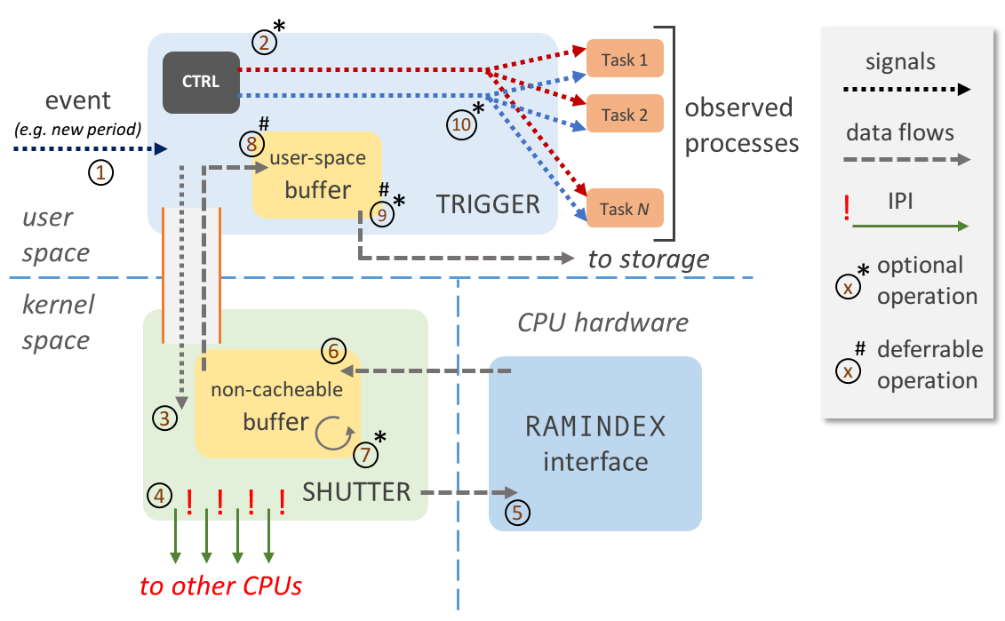
Starting from the top-level module of CacheFlow, i.e. the Trigger, we hereby review the proposed implementation following the logic flow of operations provided in Figure 2.
The Trigger module is always executed with the highest real-time priority. The module is designed for event-based activation and hence a new snapshot is initiated when a new event activates the Trigger, as shown in Figure 2. In our current prototype, we implemented two activation modes: (1) periodic activation with a configurable inter-activation time; and (2) event-based. In periodic mode, events are generated using a real-time timer set to deliver a SIGRTMAX signal to the Trigger. The tasks under analysis are launched directly by the Trigger to ensure in-phase snapshotting, and to allow the Trigger to set a specific scheduler and priority on the spawned children processes.
The Trigger implements event-based activation by initiating a snapshot upon receipt of a SIGRTMAX-1 signal. In synchronous mode, a task under analysis spawned by the Trigger can initiate a snapshot with a combination of getppid and kill system calls. This mode was used in Section VII-G to study the properties of the cache replacement policy in the target platform. The limitation of this approach is that some instrumentation in the applications’ code is required. Future extensions will leverage the ptrace family of operations to allow attaching to unmodified applications, and to trigger a new snapshot upon reaching an instruction or data breakpoint.
The next step depends on the mode (synchronous vs. asynchronous) in which the Trigger is configured to run. In the synchronous mode, the trigger immediately stops all the observed tasks with a SIGSTOP — see Figure 2. This is particularly useful if multiple cores are active, but introduces unnecessary additional overhead when performing single-core analysis. Hence, this is an optional step and skipped when the Trigger operates in asynchronous mode.
Next, the Trigger commandeers the acquisition of a new snapshot to the Shutter module via a proc filesystem interface, as depicted in Figure 2. If the trigger is operating in flush mode, the binary content of the snapshot is immediately copied to a user-space buffer via the same interface, as shown in Figure 2. At this point, the trigger might collect in-line statistics on the content of the snapshot, or (optionally) (see Figure 2) render the snapshot in human-readable format and store it in persistent memory for later analysis. This step is deferred to the end of the experiment for all the collected snapshots if CacheFlow operates in transparent mode.
Typical embedded applications make limited use of dynamic memory and dynamically linked libraries, which are instead commonly used features in general-purpose applications. It follows that the virtual memory layout — i.e. the list of VMAs — of embedded applications is generally static. It is easy to infer to which VMA a given virtual address belongs to in applications with static memory layout. Conversely, dynamically linking libraries and allocating/freeing memory at runtime can substantially change the VMA layout of an application. For this reason, the Trigger optionally allows recording the current memory layout of an application at the time a cache snapshot is acquired. This is done by reading the /proc/PID/maps interface, where PID is the process id of the application under analysis.
Finally, if the Trigger is operating in synchronous mode, a SIGCONT is sent to all the tasks under analysis as shown in Figure 2.
VI-C Shutter Implementation
The Shutter is implemented as a Linux kernel module. At startup, it establishes a communication channel with user-space by creating a new entry in the proc pseudo-filesystem. Configuration parameters and snapshot acquisition commands are sent to the Shutter via ioctl calls. If CacheFlow is operating in transparent mode, this interface is also used to specify which snapshot to retrieve at the conclusion of the experiment. A read system call (Figure 2) can be used to retrieve the selected snapshot in user-space.
Inter-CPU Synchronization: As discussed in Section V, being able to perform a full capture of L2’s content while minimizing pollution is of the utmost importance. For this reason, the Shutter delivers an Inter-Processor Interrupt (IPI) to all the other CPUs, forcing them to enter a busy-waiting loop — see Figure 2. Specifically, right before broadcasting the IPI, the Shutter acquires a spinlock. Next, the payload of the delivered IPI makes all the other CPUs wait on the spinlock.
Pollution-free Retrieval: While holding the spinlock, the Shutter proceeds to use the aforementioned RAMINDEX (see Section IV) interface to access the contents of the L2 tag memory, as shown in Figure 2. Entry by entry, a kernel-side buffer is filled with the result of the RAMINDEX operations — as per Figure 2. To avoid polluting the L2 at this step, the buffer is allocated as a non-cacheable memory region. To do so, we use the boot-time parameter mem to restrict the amount of main memory seen (and used) by Linux to carve out a large-enough physically-contiguous memory buffer. This area is then mapped by the Shutter using the ioremap_nocache kernel API and used to receive the content of the L2 tag entries.
From Physical to Virtual: After all the L2 tag entries have been retrieved, the buffer contains a collection of physical addresses, one per each cache block that was marked as valid in L2. Recall from Section V-C that operating systems that have full support for MMUs define a non-linear mapping between virtual pages and physical memory such that a set of contiguous virtual pages is comprised of arbitrarily scattered physical pages. Therefore, while the conversion virtualphysical can be easily performed using page-table walks, the reverse translation is non-trivial. The physical address resolution step depicted in Figure 2 refers to such a reverse translation performed on each of the retrieved L2 entries.
To perform this resolution, we leverage Linux’s specific representation of memory pages. Linux defines a descriptor of type struct page for each of the physical memory pages available in the system. The conversion fom physical address to page descriptor is possible through the phys_to_page kernel macro. We first derive the page descriptor of the physical address to be resolved. Next, we effectively re-purpose the reverse-map interface66 6 See https://lwn.net/Articles/75198/ for more details. (rmap) used by Linux to efficiently free physical memory when swapping is initiated. The entry point of the interface is the rmap_walk kernel API. Given a target struct page descriptor, the procedure allows one to specify a callback function to be invoked when a possible candidate for the reverse translation is found77 7 Because multiple processes might be mapping the same physical memory, the reverse translation is not always unique.. A successful rmap_walk operation returns (i) a reference to the VMA that maps the page; and (ii) the virtual address of the page inside the VMA. Importantly, the reference to the VMA allows one to derive the original memory space (struct mm_struct); and from there, the descriptor of the process (struct task_struct) associated to the memory space and its PID. After the translation step, the entries in the buffer are converted to contain two pieces of information: (i) the PID of the process to which the cache block belongs, and (ii) the virtual address of the block within the process’ virtual memory space.
The virtualphysical translation can be optionally disabled. This is useful, for instance, when profiling the cache behavior of an application pinned to a specific subset of physical pages, of a different virtual machine, or of the kernel itself.
From Kernel to User: Lastly, the contents of the kernel-side buffer are copied into a user-space buffer defined in the Trigger. On this very last step, a distinction needs to be made because the behavior of CacheFlow significantly differs when it operates in flush mode, compared to transparent mode operation.
In flush mode, the goal is to analyze what cache blocks are actively loaded by an application in between snapshots. For this reason, every snapshot acquisition is immediately followed by a copy of the snapshot to the Trigger in user-space88 8 Note that it is still important to prevent cache pollution while the current snapshot is being acquired. Thus, pollution-free retrieval is still crucial.. The Trigger also converts the binary format of the snapshot to human-readable format and writes it to disk. This step corresponds to Figure 2. The copy to user-space, as well as any post-processing performed by the Trigger, is conducted in cacheable memory. Because the amount of data moved after each snapshot is comparable in size to the L2, the post-processing acts as a tacit flush operation. However, to cope with random cache replacement policies, the Trigger performs additional cache trashing before resuming the applications to ensure that the content of the cache is indeed flushed. The presence of this flush operation is vital to the correct interpretability of the results. By doing so, each snapshot contains only cache blocks allocated during the last sampling period. Therefore, the extracted content is representative of the recent activity of the applications and enables active cache working-set analysis.
In transparent mode, the goal is to analyze the evolution of cache content over time while minimizing the impact of CacheFlow on the cache state. In this mode, no post-snapshot flush is performed. Thus, subsequent snapshots are accumulated in non-cacheable memory. They are then moved to user-space and post-processed only at the very end of the experiment. We evaluate in Section VII-C how much pollution is introduced in the various modes of operation.
Because the size of a snapshot to be transferred to user-space is on the order of hundreds of pages, we use the sequential file (seq_file) kernel interface99 9 See https://lwn.net/Articles/22355/ for more details.. This interface safely handles proc filesystem outputs spanning multiple memory pages.
VII Evaluation
This section aims to demonstrate the capabilities of the proposed and implemented CacheFlow technique. This is not meant to be an exhaustive evaluation of all the scenarios in which CacheFlow might be employed, but rather to demonstrate that CacheFlow is capable of producing useful insights on the cache usage of real applications in a real system.
VII-A Setup and Goals
All the experiments described in this section have been carried out on an NVIDIA Jetson TX1 development system running Linux v4.14. The Jetson TX1 features an NVIDIA Tegra X1 SoC, in line with what is described in Section VI.
For our workload, we use a combination of synthetic and real benchmarks. Additional details about the synthetic benchmarks we designed are provided contextually to the experiment in which they are employed. For our real benchmarks, we considered applications from the the San Diego Vision Benchmarks (SD-VBS) [40], which come with multiple input sizes. Our goal is to demonstrate the usefulness of CacheFlow in analyzing an application’s cache behavior. As such, we include only a selection of the obtained results covering the most interesting cases. We selected the Disparity, Mser, Sift, and Track benchmarks with intermediate input sizes, namely VGA (640x480) and CIF (352x288) images.
The remainder of this section is organized to address the following questions:
- 1.
Is CacheFlow able to provide an output that is representative of the actual cache behavior of an application? This is covered in Section VII-B.
- 2.
What is the overhead in terms of cache content pollution and time? We discuss this aspect in Section VII-C.
- 3.
Is it possible to track the cache behavior of real applications in term of WSS and frequently accessed memory locations using CacheFlow? We tackle this question in Section VII-D
- 4.
Can CacheFlow reveal system-level properties, such as (1) how the cache is being shared by concurrent applications; (2) how scheduling decisions impact cache usage? Section VII-E approaches this question.
- 5.
Is it possible to use CacheFlow to predict whether an application will suffer measurable cache interference from a co-running application? This is explored in Section VII-F.
- 6.
Can we study the replacement policy and implemented by the target platform and its statistical characteristics? This analysis is conducted in Section VII-G.
VII-B Is CacheFlow’s Output Meaningful?
The first aspect to validate is whether or not CacheFlow is able to provide an output that can be trusted, in the sense that it is meaningfully related to the behavior of the application under analysis. We study the output produced by CacheFlow on a synthetic benchmark. The benchmark allocates two buffers of 512 KB each. It then performs a full write followed by a full read on the first buffer. Next, it performs a full write followed by a full read on the second buffer.
We set our trigger to operate in periodic, synchronous mode, with an interval of 2 milliseconds between snapshots. We then plot a heat-map of the number of cache lines found in the snapshot for each of the pages that belong to the benchmark under analysis. We perform the experiment twice, once in flush mode and then in transparent mode. The results of the two experiments are depicted in Figure 3 and 4.


In Figure 3 we depict the heat-map for the 4 most used memory regions — as determined by reading the content of the snapshots. We only depict the most used (and interesting) region in Figure 4. The color scale we used indicates the number of lines present per 4 KB page in each snapshot, with darker blue tones indicating fewer lines and tones shifting towards yellow signifying more lines. The progression of the snapshots is plotted on the axis. Page addresses are then plotted on the axis in terms of relative offset (in pages) from the beginning of the region. We annotate the name of the region on the left-hand side of the plot.
A number of important observations can be made. We summarize the most interesting ones. First, we notice that at the beginning of the application, the pages of the stack, the text and glibc library are mostly present in cache. This is in line with the initialization of the application which uses malloc to allocate its buffer. For small allocations, malloc expands the heap of the calling process. But if the allocation of larger buffers is requested, the glibc resorts to performing a mmap call instead to create a new memory region not backed by a file (anonymous memory). It is in this anonymous region, marked as “[anon]” in the plot, that the bulk of memory accesses will be performed by our benchmark. We can also notice that the region comprises 256 pages, i.e. 1 MB.
Let us now focus on this region. In Figure 3, one can easily distinguish the scan performed by the benchmark over the buffers. Each scan shows up as bands of yellow moving left-to-right. Because a full pass of stores followed by a full pass of loads is performed in each scan, two yellow bands are visible in each scan. By looking at the slope of these bands, it is possible to understand the rate of progress of the benchmark moving through the buffer. It can be noted that stores are slower than loads — it takes around 8 snapshots to complete the first store sub-iteration, and only 5 for the loads. This might sound counter-intuitive but indeed makes sense because (1) in write-back caches a store might result in a write-back of a dirty line followed by a load from main memory; and (2) a cache with many outstanding store transactions will stall when its internal write-buffer is full.
Because Figure 3 was produced in flush mode, the only cache lines highlighted in the heat-map are those that were accessed by the application in-between snapshots. It goes to demonstrate that flush mode is particularly well suited to study the active cache set of applications. Conversely, operating in transparent mode allows us to understand how/if cache lines allocated at some point during execution persist in cache. Figure 4 depicts one such case. After snapshot 12, the application will not access the top portion of its addressing space. Nonetheless, since the overall buffer touched by the application is smaller than the cache size, the unused lines remain in cache. These lines slightly fade in color because some eviction still occurs due to the random replacement policy of this cache.
VII-C What is the Overhead of Snaphotting?
We evaluate the overhead introduced by CacheFlow along two dimensions: cache pollution and timing. We measure cache pollution as the change in cache content that is introduced solely because of CacheFlow’s activity. To evaluate cache pollution, we first execute a cache-intensive application for a given lead time set to 100 ms. The lead time allows the application to populate the cache. Then, we set the Trigger to activate at the end of the lead time and to acquire two consecutive snapshots back-to-back. The first snapshot captures the content of the cache status as populated by the application under analysis. The second snapshot is used to understand the change in cache status introduced by kernel-to-user copy of the first snapshot and its post-processing. The overhead then is evaluated in terms of percentage of cache lines that have changed over the total number of cache lines. The overhead in time is evaluated by measuring the end-to-end time required to acquire a single snapshot.
| Space Overhead (%) | Time Overhead ( Cycles) | |||||
|---|---|---|---|---|---|---|
| Mode | Avg. | Std. Dev | Max | Avg. | Std. Dev. | Max |
| Full Flush | 95.23 | 3.21 | 99.10 | 10.13 | 0.78 | 12.88 |
| Resolve+Layout | 13.40 | 0.43 | 14.70 | 0.34 | 0.00 | 0.35 |
| Resolve | 6.78 | 0.45 | 8.23 | 0.34 | 0.00 | 0.34 |
| Layout | 6.55 | 0.50 | 8.71 | 0.20 | 0.00 | 0.20 |
| Full Transparent | 1.06 | 0.19 | 1.38 | 0.19 | 0.00 | 0.19 |
The results of the overhead measurements are reported in Table II and are the aggregation of 100 experiments for each setup. We measure pollution and time overhead in synchronous mode because it is the most suitable for general analysis scenarios. We then consider a host of different sub-modes. In “Full Flush”, CacheFlow operates in flush mode with physicalvirtual translation and VMA layout acquisition active. As expected, around 95% of the cache content is modified in this mode after a snapshot is completed. The next four cases correspond to the overhead of CacheFlow operating in transparent mode. In the “Resolve+Layout” mode, both address resolution and VMA layout acquisition are turned on. In the “Resolve” (resp., “Layout”) case, only address resolution (resp., VMA layout acquisition) are enabled. Finally in the “Full Transparent” case, both address resolution and VMA layout acquisition are skipped. Notably, cache pollution in full transparent mode does not exceed 1.4%, which is acceptable for a software-only solution. Times are reported in millions of CPU cycles to better generalize to other platforms. The CPUs operate at 1.9 GHz on the target platform.
VII-D Can CacheFlow Analyze Real Applications?
Having assessed that CacheFlow can indeed provide accurate insights into an application’s cache utilization, we analyze two real applications. Figure 5 and Figure 6 report the heat-map analysis of SD-VBS benchmarks Disparity and Sift, respectively, using VGA resolution images in input.
It can be observed that Disparity is characterized by quite distinguishable intro (snap. 0-25) and outro phases (snap. 172-198). In the intro, the input buffer is first pre-processed in the “anon” region. It follows an intermediate processing phase that actively uses around 83% of the region’s memory with a recurring pattern and pages with offset 466-930 being the most frequently accessed. During the outro phase the final output is produced sequentially on the heap. A quite different picture is painted by the Sift application. In this case, there exists an initial phase (snap. 0-40) where pre-processing is performed on an anonymous region; then the bulk of processing is carried out on the heap. From around snapshot 30 until 170, two non-contiguous sets of memory pages are in use, that gradually span through 82% of the region. The final computation step is performed on the top 75% of the heap.


VII-E Can CacheFlow Discover System Properties?
CacheFlow can also provide valuable insights on the cache-related behavior of the whole system when multiple applications are executed. To evaluate this, we concurrently run four SD-VBS applications, namely Track, Mser, Sift, Disparity, all with VGA resolution images in input.
In the first experiment, the benchmarks are executed on a single core — the other three cores are turned off. Moreover, the default Linux’s scheduling policy (SCHED_OTHER) is used. We then set the Trigger to acquire periodic snapshots every 10 ms and study the per-process L2 occupancy over time. The results are shown in Figure 7. The SCHED_OTHER scheduler implements a Completely Fair Scheduler (CFS), which tries to ensure an even progress of co-running workload. This results in frequent context-switches that result in quick changes in the composition of the L2 cache content visible in the figure. The figure also shows how more cache-intensive benchmarks such as Disparity can dominate other workload in terms of utilization of cache resources.
To understand the impact of scheduling policies on cache utilization, we conduct a similar experiment where we use a fixed-priority real-time scheduler. Specifically, we run the benchmarks with SCHED_FIFO policy and set their priorities to be in decreasing order — i.e. Track has highest priority, Disparity has lowest priority. With this setup, we obtain Figure 8. In this case, it is clear that the execution of the benchmarks is performed in strict order with no interleaving. It can also be noted how the benchmarks under analysis vary their WSS as they progress. Another interesting observation is that overall the execution takes less time (640 snapshots) compared to Figure 7, likely due to better cache locality in absence of frequent context switching.
Next, we demonstrate that CacheFlow can also be used to investigate the behavior of the shared L2 cache even with multiple cores being active. In this setup, we turn on 3 out of 4 cores1010 10 We also conducted the experiment on the full 4-core setup, which yielded similar results and is omitted due to space constraints. and deploy the same set of 4 SD-VBS benchmarks with the arrangement of real-time priorities. We do not control process-to-CPU assignment and let the Linux scheduler allocate processes to cores at runtime. What emerges in terms of per-process L2 occupancy is depicted in Figure 9. Given that L2 is a shared cache, we see multiple applications competing for cache space. As they progress, the amount of occupied cache depends not only on their current WSS, but also on the WSS of co-running applications. This is particularly clear when looking at the interplay in cache between the Track and Mser benchmarks compared to what we observed in Figure 8. Because only 3 cores are available, it can also be noted that Disparity only starts executing at snapshot 68, once again significantly dominating cache utilization in the central portion of its execution (snap. 98-215).
VII-F Can Clash on Shared Cache be Predicted?
In this section, we investigate if cache snapshotting can be used to predict clash on cache resources between co-running applications. To conduct this analysis, we first analyze the behavior of our applications in isolation. We use snapshotting to derive two type of profiles on the SD-VBS applications under analysis. Both profiles are constructed from snapshots acquired in flush mode. In the first profile, we study the sheer size of data allocated in cache at each snapshot — “Active” set analysis. In the second type of profile, namely “Reused” set analysis, we evaluate only the number of lines that are the same and present in two successive snapshots. The reused set captures the amount of data that, if evicted, causes a penalty in execution time. While active set analysis could be carried out by carefully interpreting cache performance counters, reused set analysis can only be conducted by leveraging the exact knowledge of what lines are cached from time to time. Hence, this type of analysis was previously limited to simulation studies.
Figure 10 depicts the two profiles for each of the considered real benchmarks. In addition, we considered a synthetic benchmark called Bomb which continually and sequentially accesses a 2.5 MB buffer. From the figure, it appears that while there exists a positive correlation between the active and reuse set, the two often (and substantially) differ.
Using the profiles, we build two metrics to try and predict the impact that two applications running in parallel would have on each other. For this experiment, we establish the ground truth by observing the slowdown suffered by an application under analysis when running in parallel with an interfering application. In these measurements, CacheFlow is not used. The results are reported in Table III, in the first group of rows.
The first metric, namely “Active Set Excess” is based on active sets only. In this case, we consider two applications at a time: an observed, and an interfering one. We then consider the sum of their active sets on a per-snapshot basis, and compute how much that sum exceeds the size of the cache (e.g. by 0%, by 50% etc.). We then average this quantity over the full length of the profile. The results obtained from applying this metric on all the considered SD-VBS applications are reported in Table III — second group of rows.
A second metric, namely “Reused Set Eviction”, considers how much of the reused set of the application under analysis is potentially evicted by an interfering application. To build this metric, we once again reason on a per-snapshot basis. We multiply the reused set quota of the application under analysis by the active set quota of the interfering application. The average over the full length of the profile is then computed. The third group of rows in Table III reports the reused set eviction metric computed for the considered benchmarks.
Finally, we computed the correlation between the two metrics described above and the ground truth on the measured slowdown. The reused set eviction metric revealed an 80% correlation with slowdown. It outperformed the active set excess metric which achieved 74% correlation. These results serve as a proof-of-concept that CacheFlow can be used, for instance, to perform interference-aware scheduling decisions.
| Benchmark Under Analysis | |||||
| Interf. Applic. | Disparity | Mser | Sift | Track | |
| Disparity | 1.16 | 1.13 | 1.02 | 1.02 | |
| Mser | 1.02 | 1.06 | 1.01 | 1.02 | |
| Sift | 1.03 | 1.05 | 1.05 | 1.06 | |
| Track | 1.01 | 1.02 | 1.03 | 1.06 | |
| Slowdown () | Bomb | 1.12 | 1.20 | 1.05 | 1.04 |
| Disparity | 0.55 | 0.33 | 0.19 | 0.19 | |
| Mser | 0.12 | 0.25 | 0.04 | 0.03 | |
| Sift | 0.24 | 0.14 | 0.14 | 0.07 | |
| Track | 0.12 | 0.05 | 0.04 | 0.15 | |
| Bomb | 0.64 | 0.42 | 0.46 | 0.31 | |
| Active Set Excess (%) | Correlation: | 0.74 | |||
| Disparity | 0.15 | 0.12 | 0.08 | 0.07 | |
| Mser | 0.03 | 0.10 | 0.02 | 0.01 | |
| Sift | 0.08 | 0.08 | 0.07 | 0.04 | |
| Track | 0.04 | 0.04 | 0.03 | 0.06 | |
| Bomb | 0.18 | 0.15 | 0.13 | 0.09 | |
| Reused Set Eviction (%) | Correlation: | 0.80 | |||
VII-G Can we Study the Cache Replacement Policy?
The last aspect we evaluated was the capability introduced by CacheFlow to evaluate the replacement policy implemented by the hardware. We focus on two aspects. First, we validate that the policy indeed follows random replacement. Second, we study how well the implemented replacement policy matches a truly random replacement. To conduct these experiments we devised a special synthetic benchmark, namely Repl. The Repl benchmark allocates from user-space a set of contiguous physical pages with a total size equal to the L2 cache size. This is done by mmap leveraging support for huge pages — MAP_HUGE_2MB flag.
Because the allocated buffer is aligned with the cache size, the first line, say Line , of the buffer necessarily maps to cache set 0. Similarly, the line (Line ) that is exactly 128 KB away (the size of one cache way) from Line also maps to set 0. With a similar reasoning we identify a set of 16 lines that map to set 0. If the cache implements a deterministic cache replacement policy (e.g. LRU or FIFO), then accessing lines through will result in a snapshot containing all the lines. Following this idea, the Repl benchmark touches lines through a configurable number of times (iterations). Then, it delivers a signal to the Trigger (event-based activation) to acquire a snapshot in transparent mode. In the snapshot, we evaluate how many of the 16 lines are actually present in cache. By repeating the same experiment 1000 times, we can plot the probability density that out of 16 lines are found in cache. We repeat the experiment by performing from 1 to 8 iterations over lines through before acquiring a snapshot. The resulting density plots are reported in Figure 11.
In our last experiment, we evaluate how closely the implemented random replacement policy matches a truly random replacement policy. To evaluate this aspect, we use a variant of the Repl benchmark. We consider again lines through . But in this case, the benchmark activates the Trigger after touching each line and stops after reaching line . A single run produces 16 snapshots. Moreover in snapshot 1, we can derive which cache way was selected to allocate , in snapshot 2 what way was selected for and so on. We run the experiment 2000 times and collect a total of 32,000 replacement decisions. We then compute the number of times each of the 16 cache ways were selected for allocation over the total number of observations. The results are reported in Figure 12. In a perfect random replacement scheme, each way has probability of being selected. The implemented replacement policy does not deviate significantly from a perfect replacement, although interestingly, it appears that the central ways (ways 7 to 11) are statistically less likely to be selected for allocation.
VIII Conclusion and Future Work
In this work, we have proposed a technique, namely CacheFlow, that leverages existing yet untapped micro-architectural support to enable cache content snapshotting. The proposed implementation has highlighted that CacheFlow can provide unprecedented insights on application-level features in the usage of cache resources, and on system-level properties. As such, we envision that CacheFlow and its analogues will serve as a powerful instrument for system designers to better understand the interplay between applications, system components, and cache hierarchy. Ultimately, we expect that it will complement existing simulation-based and static analysis approaches by providing a way to refine and validate cache memory models. While we have restricted ourselves to analyzing the LLC in this work, RAMINDEX’s capabilities far exceed that. Hence, we encourage the community to extend and refine the proposed open-source implementation to conduct a wider range of studies, e.g. on the behavior of private caches, TLBs, and coherence controllers.
References
- [1] M. Lv, N. Guan, J. Reineke, R. Wilhelm, and W. Yi, “A survey on static cache analysis for real-time systems,” Leibniz Transactions on Embedded Systems, vol. 3, no. 1, pp. 05–1, 2016.
- [2] R. Wilhelm, J. Engblom, A. Ermedahl, N. Holsti, S. Thesing, D. Whalley, G. Bernat, C. Ferdinand, R. Heckmann, T. Mitra et al., “The worst-case execution-time problem—overview of methods and survey of tools,” ACM Transactions on Embedded Computing Systems (TECS), vol. 7, no. 3, pp. 1–53, 2008.
- [3] D. Grund, Static Cache Analysis for Real-Time Systems: LRU, FIFO, PLRU. epubli, 2012.
- [4] C. Ferdinand and R. Wilhelm, “Efficient and precise cache behavior prediction for real-time systems,” Real-Time Systems, vol. 17, no. 2-3, pp. 131–181, 1999.
- [5] P. Cousot and R. Cousot, “Basic concepts of abstract interpretation,” in Building the Information Society. Springer, 2004, pp. 359–366.
- [6] R. T. White, F. Mueller, C. A. Healy, D. B. Whalley, and M. G. Harmon, “Timing analysis for data caches and set-associative caches,” in Proceedings Third IEEE Real-Time Technology and Applications Symposium. IEEE, 1997, pp. 192–202.
- [7] J. Reineke, D. Grund, C. Berg, and R. Wilhelm, “Timing predictability of cache replacement policies,” Real-Time Systems, vol. 37, no. 2, pp. 99–122, 2007.
- [8] N. Guan, X. Yang, M. Lv, and W. Yi, “FIFO cache analysis for wcet estimation: A quantitative approach,” in 2013 Design, Automation & Test in Europe Conference & Exhibition (DATE). IEEE, 2013, pp. 296–301.
- [9] D. Grund and J. Reineke, “Precise and efficient fifo-replacement analysis based on static phase detection,” in 2010 22nd Euromicro Conference on Real-Time Systems. IEEE, 2010, pp. 155–164.
- [10] D.-H. Chu and J. Jaffar, “Symbolic simulation on complicated loops for wcet path analysis,” in 9th ACM International Conference on Embedded Software (EMSOFT). IEEE, 2011, pp. 319–328.
- [11] D. Chu, J. Jaffar, and R. Maghareh, “Precise cache timing analysis via symbolic execution,” in 2016 IEEE Real-Time and Embedded Technology and Applications Symposium (RTAS), 2016, pp. 1–12.
- [12] N. Binkert, B. Beckmann, G. Black, S. K. Reinhardt, A. Saidi, A. Basu, J. Hestness, D. R. Hower, T. Krishna, S. Sardashti, R. Sen, K. Sewell, M. Shoaib, N. Vaish, M. D. Hill, and D. A. Wood, “The gem5 simulator,” SIGARCH Comput. Archit. News, vol. 39, no. 2, p. 1–7, Aug. 2011. [Online]. Available: https://doi.org/10.1145/2024716.2024718
- [13] S. R. Sarangi, R. Kalayappan, P. Kallurkar, S. Goel, and E. Peter, “Tejas: A java based versatile micro-architectural simulator,” in 2015 25th International Workshop on Power and Timing Modeling, Optimization and Simulation (PATMOS), 2015, pp. 47–54.
- [14] J. Wang, J. Beu, R. Bheda, T. Conte, Z. Dong, C. Kersey, M. Rasquinha, G. Riley, W. Song, H. Xiao, P. Xu, and S. Yalamanchili, “Manifold: A parallel simulation framework for multicore systems,” in 2014 IEEE International Symposium on Performance Analysis of Systems and Software (ISPASS), 2014, pp. 106–115.
- [15] N. Nethercote and J. Seward, “Valgrind: A program supervision framework,” Electronic notes in theoretical computer science, vol. 89, no. 2, pp. 44–66, 2003.
- [16] Z. Wang and J. Henkel, “Fast and accurate cache modeling in source-level simulation of embedded software,” in 2013 Design, Automation & Test in Europe Conference & Exhibition (DATE). IEEE, 2013, pp. 587–592.
- [17] L. M. N. Coutinho, J. L. D. Mendes, and C. A. P. S. Martins, “Mscsim -multilevel and split cache simulator,” in Proceedings. Frontiers in Education. 36th Annual Conference, Oct 2006, pp. 7–12.
- [18] S. E. Arda, A. NK, A. A. Goksoy, N. Kumbhare, J. Mack, A. L. Sartor, . A. Akoglu, R. Marculescu, and U. Y. Ogras, “Ds3: A system-level domain-specific system-on-chip simulation framework,” 2020.
- [19] H. Brais, R. Kalayappan, and P. R. Panda, “A survey of cache simulators,” ACM Comput. Surv., vol. 53, no. 1, Feb. 2020.
- [20] N. Nethercote and J. Seward, “Valgrind: A framework for heavyweight dynamic binary instrumentation,” in Proceedings of the 28th ACM SIGPLAN Conference on Programming Language Design and Implementation, ser. PLDI ’07. New York, NY, USA: Association for Computing Machinery, 2007, p. 89–100.
- [21] D. Levinthal, “Performance analysis guide for intel core i7 processor and intel xeon 5500 processors,” Intel Performance Analysis Guide, vol. 30, p. 18, 2009.
- [22] J. Treibig, G. Hager, and G. Wellein, “Performance patterns and hardware metrics on modern multicore processors: Best practices for performance engineering,” in European Conference on Parallel Processing. Springer, 2012, pp. 451–460.
- [23] D. Molka, R. Schöne, D. Hackenberg, and W. E. Nagel, “Detecting memory-boundedness with hardware performance counters,” in Proceedings of the 8th ACM/SPEC on International Conference on Performance Engineering, ser. ICPE ’17. New York, NY, USA: Association for Computing Machinery, 2017, p. 27–38.
- [24] P. J. Mucci, S. Browne, C. Deane, and G. Ho, “PAPI: A portable interface to hardware performance counters,” in Proceedings of the department of defense HPCMP users group conference, vol. 710, 1999.
- [25] S. Browne, J. Dongarra, N. Garner, G. Ho, and P. Mucci, “A portable programming interface for performance evaluation on modern processors,” The international journal of high performance computing applications, vol. 14, no. 3, pp. 189–204, 2000.
- [26] J. Treibig, G. Hager, and G. Wellein, “Likwid: A lightweight performance-oriented tool suite for x86 multicore environments,” in 2010 39th International Conference on Parallel Processing Workshops. IEEE, 2010, pp. 207–216.
- [27] M. Selva, L. Morel, and K. Marquet, “numap: A portable library for low-level memory profiling,” in 2016 International Conference on Embedded Computer Systems: Architectures, Modeling and Simulation (SAMOS). IEEE, 2016, pp. 55–62.
- [28] A. Vishnoi, P. R. Panda, and M. Balakrishnan, “Online cache state dumping for processor debug,” in Proceedings of the 46th Annual Design Automation Conference, 2009, pp. 358–363.
- [29] B. R. Buck and J. K. Hollingsworth, “A new hardware monitor design to measure data structure-specific cache eviction information,” The International Journal of High Performance Computing Applications, vol. 20, no. 3, pp. 353–363, 2006.
- [30] P. R. Panda, A. Vishnoi, and M. Balakrishnan, “Enhancing post-silicon processor debug with incremental cache state dumping,” in 2010 18th IEEE/IFIP International Conference on VLSI and System-on-Chip. IEEE, 2010, pp. 55–60.
- [31] ARM Holdings, “Cortex-A53 MPCore technical reference manual (r0p4),” 2018.
- [32] ——, “Cortex-A57 MPCore technical reference manual (r1p3),” 2016.
- [33] ——, “Cortex-A72 MPCore technical reference manual (r0p2),” 2016.
- [34] ——, “Cortex-A15 technical reference manual (r2p0),” 2011.
- [35] ——, “Cortex-A9 technical reference manual (r4p0),” 2009.
- [36] J. Corbet, J. Edge, and R. Sobol, “Kernel Development,” Linux Weekly News – https://lwn.net/Articles/74295/, 2004, [Online; accessed 7-May-2019].
- [37] ARM Holdings, “Cortex‑A76 Core technical reference manual (r3p0),” 2018.
- [38] ——, “Cortex‑A77 Core technical reference manual (r1p1),” 2019.
- [39] Nvidia Corporation, “NVIDIA Tegra X1 Technical Reference Manual,” https://developer.nvidia.com/embedded/tegra-2-reference.
- [40] S. K. Venkata, I. Ahn, D. Jeon, A. Gupta, C. Louie, S. Garcia, S. Belongie, and M. B. Taylor, “SD-VBS: The san diego vision benchmark suite,” in 2009 IEEE International Symposium on Workload Characterization (IISWC), Oct 2009, pp. 55–64.