Noise and ergodic properties of Brownian motion in an optical tweezer: looking at the crossover between Wiener and Ornstein-Uhlenbeck processes
Abstract
We characterize throughout the spectral range of an optical trap the nature of the noise at play and the ergodic properties of the corresponding Brownian motion of an overdamped trapped single microsphere, comparing experimental, analytical and simulated data. We carefully analyze noise and ergodic properties using the Allan variance for characterizing the noise and exploiting a test of ergodicity tailored for experiments done over finite times. We derive these two observables in the low-frequency Ornstein-Uhlenbeck trapped-diffusion regime and study analytically their evolution towards the high-frequency Wiener free-diffusion regime, in a very good agreement with simulated and experimental results. This leads to reveal noise and ergodic spectral signatures associated with the distinctive features of both regimes.
I Introduction
The high sensitivity of optically trapped Brownian particles, combined with long integration times available, makes optical traps outstanding metrological systems. They have therefore been involved in many weak force experiments and have been recognized as outstanding systems for implementing and simulating many results and protocols that have been brought forward recently in the field of optomechanics and non-equilibrium statistical physics Ciliberto 2017; Martinez et al. 2017; Bechhoefer et al. 2020.
Optical traps physically implement an Ornstein-Uhlenbeck process through the harmonic trapping force field. One of their interesting features is to give access to different diffusing dynamics for the trapped Brownian object, ranging from confined motion in the long timescales to free Brownian motion on the shortest ones, therefore probing the evolution of the Ornstein-Uhlenbeck process towards the Wiener process-like limit at short times Uhlenbeck and Ornstein 1930; Gardiner 2009. These two dynamic regimes have very different properties that make them more relevant for different experiments. In particular, the Ornstein-Uhlenbeck regime is well suited for force measurements Wu et al. 2009; Ether et al. 2015; Ricci et al. 2017; Li et al. 2019 while position detection benefits from the Wiener regime, allowing to achieve higher resolution Lukić et al. 2005; Li et al. 2010; Schnoering et al. 2019.
In this article, we address these differences from the viewpoints of noise stability and ergodicity for both regimes. We implement theoretical and experimental tools capable of characterizing motional noise (using an Allan-variance based analysis Czerwinski et al. 2009; Lansdorp and Saleh 2012) and ergodic signatures (developing a specific test of ergodicity Metzler et al. 2014; Cherstvy and Metzler 2015) in an optical trap from the Ornstein-Uhlenbeck regime to its high frequency Wiener limit in a unified way.
This capacity is important in particular in the field of precision measurements involving optical traps. There indeed, the building of large motional statistical ensembles necessary to reach high resolution levels usually relies on strong assumptions related to the nature and stability of the driving noise. It also depends on the ergodicity of the corresponding Brownian motion. We show here precisely how these assumptions can be tested on overdamped harmonic optical traps, paving the way for reliable experiments at all measurement bandwidths. The tools we describe below are general: they can be used on underdamped and more complex systems and can thereby be exploited when colored noise and non-ergodic effects enrich the physics of Brownian motion, as in the realm of swimmers or active matter, for instance.
II Wiener vs. Ornstein-Uhlenbeck crossover in an optical trap
Free Brownian motion driven only by the Gaussian white noise of thermal fluctuations is described by the Wiener process . The displacement of the overdamped free Brownian object writes as:
| (1) |
working directly with the differential with the following properties: , .The diffusion coefficient involves the Boltzmann constant , the temperature of the surrounding fluid and the Stokes drag coefficient .
Inside the trap, the harmonic optical potential modifies the stochastic process by exerting on the object a restoring force characterized by a constant stiffness . The same displacement now follows the Ornstein-Uhlenbeck process:
| (2) |

Our experiment, detailed in Appendix A, consists in trapping a single Brownian object in the harmonic potential created at the waist of a focused laser beam, and recording the instantaneous overdamped position of the trapped bead, as schematized in Fig. 1. All the experimental results presented in this work are obtained from a 10 minutes long trajectory (i.e. successive position measurements acquired at a frequency of Hz).
These data are compared, throughout this article, with numerical simulations obtained from an algorithm for the Wiener process:
| (3) |
where is a dimensionless Gaussian white noise with , , according to the methods detailed in Volpe and Volpe 2013. By the same token, the algorithm for the Ornstein-Uhlenbeck process is:
| (4) |
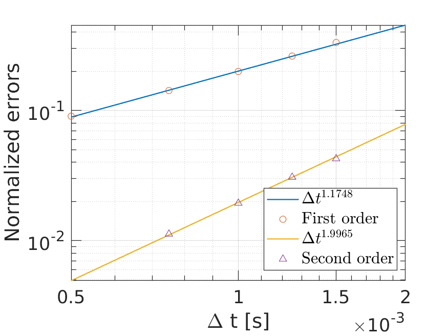
This discretisation method, known as the Euler-Maruyama method, corresponds to an approximation of Itô-Taylor expansions Kloeden and Platen 1992. As discussed in details in Appendix D, higher order terms lead to a more efficient algorithm known as the Mildstein algorithm, which our simulations are based on and which converges more quickly towards the analytical expression as decreases Higham 2001; Vanden-Eijnden and Ciccotti 2006.
From Eq. (2), the Brownian motion in the trap can be spectrally analyzed with the position’s power spectral density (PSD):
| (5) |
As clearly seen on the experimental PSD displayed in Fig. 2, the roll-off frequency separates the high frequency regime of free Brownian motion -see Eq. (1)- from the low frequency trapping regime -see Eq. (2). The PSD thus clearly reveals how a Wiener regime corresponds in the optical trap to the short time limit of the Ornstein-Uhlenbeck process (in other words, when observed over such a short timescale, the Brownian object moves inside the trap as if it were freely diffusing without confinement).

III Noise stability: Allan variance and statistical tests
In order to characterize the noise at play inside the optical trap, it is central to measure two of its properties: its nature (color, thermal weight, frequency contributions, etc), and its stability in time. Testing the nature of the noise can be done spectrally with the PSD that yields the different frequency contributions of the noise. Integrated PSD can also reveal the thermal nature of the noise through the fluctuation-dissipation theorem. However, the spectral approach turns out to be exposed to possible low frequency drifts that can modify noise properties Li et al. 2019; Czerwinski et al. 2009; Lansdorp and Saleh 2012. In order to avoid this stability issue, we work in the time-domain and perform an Allan-variance based test of the system, capable of revealing low frequency drifts within a stochastic signal Allan 1966; Barnes et al. 1971. This approach leads us to verify unambiguously the stationary and thermally limited properties of the noise at play in an experiment.
The Allan variance can be connected to the noise PSD through the following relation Barnes et al. 1971:
| (6) |
It can therefore be explicitly evaluated analytically for the Ornstein-Uhlenbeck PSD of Eq. (5):
| (7) |
as detailed in Appendix E.
The experimental Allan variance is shown in Fig. 3 following the same methodology presented in our earlier work Li et al. 2019. This experimental Allan variance is compared with numerical simulations and with the analytical result of Eq. (7). We note a remarkable experiment-theory agreement over more than 6 decades in time. These results show the very high level of noise stability up to s that one can reach on a simple optical trap setup such as ours.
But they also reveal how the Ornstein-Uhlenbeck and the Wiener processes are characterized by different Allan variance signatures. Indeed, we identify here two clear asymptotic regimes. The short time regime () falls on the slope, which is known to corresponds to the thermal white noise limit of free Brownian motion Czerwinski et al. 2009; Li et al. 2019. Interestingly, in the long time limit () of the Ornstein-Uhlenbeck process where the trapping action dominates the motional dynamics, the Allan variance shows a different slope with . This change of signatures between the two regimes, accounting for the presence of the harmonic force field in the long time limit, is continuous. We observe a very good match between the experiments and theory in the transition between asymptotic regimes.
The slight differences at short time-lags between the theory and the experimental data will also be observed at the level of the mean squared displacement (MSD) Fig. 4 (a) and the ergodic parameter Fig. 5. As discussed in details in Appendix G, these deviations are due to tracking errors unavoidably induced experimentally by the photodiode and electronic system used for recording our Brownian trajectories.

We will now use an alternative method based on the autocorrelation and the MSD for identifying either a Wiener or an Ornstein-Uhlenbeck process. We however remind here that at thermal equilibrium, Wiener and Ornstein-Uhlenbeck processes generate trajectories with different statistical properties. Indeed, the Ornstein-Uhlenbeck process of the trapped Brownian motion has a variance constant in time with the equipartition condition . In contrast, the Wiener process of free Brownian motion is non-stationary with a motional variance that grows linearly in time. But looking at the statistical properties of successive displacements whose dynamics is governed by Eqs. (1,2), it becomes possible to perform the same stationarity test for both processes. To do that, we will use the autocorrelation of displacements and the MSD, extracted from long trajectories. We will verify stationarity –in the strong sense since the noise is Gaussian– with a fixed mean (that can be removed without any loss of generality), a finite variance , and a displacement covariance (autocorrelation) that depends only on the absolute time difference .
The covariance of displacements can be computed using Eq. (2) (details are given in Appendix B, see Eq. (21)) and yields:
| (8) |
This theoretical expression is compared to the covariance evaluated experimentally as a time-average on successive displacements. The comparison, together with simulations, is shown on figure 4 (a). The convergence of the time averaging process for the covariance towards the theoretical expression, only function of , shows the absence of dependence on the absolute time .
We can also evaluate the MSD directly from the measurement of successive positions separated by a given time-lag (details are given in Appendix C, see Eq. (25)) as:
| (9) |
Again, this theoretical result is compared to the experimental MSD which is given by evaluating the time average MSD of the entire trajectory. The comparison, also including simulations, shows a very good agreement displayed in Fig. 4 (b).
This agreement, together with the covariance, depending only on time-difference, confirms that our Brownian trap implements a strong stationary Ornstein-Uhlenbeck process. Clearly, our data demonstrate a smooth crossover between the linear MSD at short time lags associated with a Wiener regime and the constant MSD at longer time lags that reflects the confined nature of the diffusion for the Ornstein-Uhlenbeck process.


IV Test of ergodicity
As reminded in the Introduction, the ergodic hypothesis is central for reaching high resolution levels in optical trapping experiments. Ergodicity per se corresponds to the equality taken in the infinite time limit , between the time average and the ensemble average for a given stochastic process. In order to test ergodicity, we first need to build an ensemble of trajectories . To do this, we reshape our long trajectory into an ensemble of 600 trajectories of 1 second duration each. For such a trajectory drawn from the ensemble, ergodicity is defined as:
| (10) |
Although simple, this definition is however hardly operative in experiments that only yield ensembles of finite-time trajectories. Following the approach proposed in Metzler et al. 2014; Cherstvy and Metzler 2015, we prefer resorting to an observable that can characterize the ergodic nature of an experiment performed over a finite integration time. This observable is grounded on the stationary nature of the MSD which is, as we shown above, independent of the choice from the initial time and only depends on the time-lag . In such conditions, ergodicity simply demands the time average MSD of any -trajectory, as defined above, to be equal, in the long limit, to the ensemble mean of individual time average taken over the ensemble of available trajectories:
| (11) |
Formally, ergodicity demands that the ratio tends to a Dirac distribution as . A sufficient condition for ergodicity is therefore that the normalized variance of this ratio goes to zero in the limit :
| (12) |

Handling therefore finite integration times, this normalized variance is the right observable needed to prove the ergodic nature of a stochastic process experimentally implemented. One very appealing aspect of is that it can be theoretically calculated for an Ornstein-Uhlenbeck process, as we do in Appendix F. This gives the capacity to characterize the ergodicity throughout the spectral range of the optical trap, therefore both in the long-time trapped and the short-time free diffusion regimes. These two regimes correspond to different time-lag evolutions of , as clearly seen in Fig. 5. Here too, a smooth crossover between the long time-lag trapped (Ornstein-Uhlenbeck) regime and the short time-lag free (Wiener limit) regimes is revealed and measured, with the transition time-lag determined from the trap stiffness, as discussed in more details in Appendix F. The experimental evolution of corresponding to the recorded finite-time trajectories obtained for our trapping experiment is also shown. The excellent agreement with the theoretical in both the freely diffusing and in the trapped regimes confirms that our optical trapping process can be considered as ergodic with a high level of confidence. Because is formally a variance, the quality of its estimator on a finite-size ensemble can be quantified using a -test. We perform in Fig. 5 this test up to a level of confidence.
V Conclusion
By implementing in a combined manner Allan variance-based, stationarity and ergodic tests, we have been able to fully characterize, through wide spectral ranges, the nature of the noise and the ergodicity of the stochastic regimes at play in our overdamped optical trap. In particular, our observables have revealed distinctive features between the high and low frequency range of the trap. There are clear differences from the viewpoint of noise stability and ergodicity between Wiener and Ornstein-Uhlenbeck processes notwithstanding that they are driven by the same Gaussian white thermal noise. These differences appear in our results when comparing the different dynamical regimes. In stochastic thermodynamics, ergodic processes are a very important subclass of stationary processes. When aiming at exploiting Brownian systems, it is therefore very important to be able to identify stationarity signatures. The simple and straightforward methodology proposed in our work is also relevant to many recent experiments involving Brownian systems coupled to non-thermal, colored, and more complex noise environments Bechinger et al. 2016.
VI Acknowledgements
Thanks are due to A. Canaguier-Durand and G. Schnoering for stimulating discussions. This work was supported in part by Agence Nationale de la Recherche (ANR), France, ANR Equipex Union (Grant No. ANR-10-EQPX-52-01), the Labex NIE projects (Grant No. ANR-11-LABX-0058-NIE), and USIAS within the Investissements d’Avenir program (Grant No. ANR-10-IDEX- 0002-02).
Appendix A Experimental setup
Our experiment consists in trapping a single Brownian object in the harmonic potential created at the waist of a focused laser beam. A schematic view of the setup is given on Fig. 6. A linearly polarized Gaussian beam (OBIS Coherent, CW 785 nm, 110mW) is focused by a water immersion objective (Nikon Plan Apochromat , Numerical Aperture ) into the sample that consists in a cell made of a glass slide and a coverslip, separated by a m thick and cm wide spacer. The cell is filled with a colloidal dispersion of polystyrene microspheres (ThermoFisher FluoSpheres polystyrene microspheres, m diameter ) diluted in deionised water. We start with a solution of concentration of beads/mL that we dilute . The cell is then taped to a metallic holder mounted in our optical setup.

The instantaneous position of the trapped single bead is recorded using an additional low-intensity counter-propagating laser beam (Thorlabs HL6323MG CW nm, 30 mW, but here used at low power), focused on the bead using a second objective (Nikon Plan-fluo Extra Large Working Distance , Numerical Aperture ). Within the small trapping volume defined by our setup, the intensity of the light scattered by the microsphere scales linearly with its displacement along the optical axis. This scattered intensity signal is collected through the trapping objective and sent to a P.I.N. photodiode (Thorlabs, model Det10A2). The output signal recorded in V is sent to a low noise amplifier (Stanford Research, SR560) and then acquired by an analog-to-digital card (National Instrument, PCI-6251). The signal is filtered through a Hz high-pass filter at 6 dB/oct in order to remove the DC component of the output signal and through a kHz low-pas filter at 6 dB/oct to prevent aliasing. Finally, we convert the voltage signal into displacements measured in m.
In our experiment, it is crucial to trap only one bead at a time. To achieve this, we rely on a low concentration of beads in the solution and a direct imaging of the vicinity of the trap with an Interferometric scattering microscopy technique (not shown on the figure but presented in details in our previous work Schnoering et al. 2018). A second important point is ensured by the thickness (m) of the cell : the trapping region must be localized far enough from the walls as to keep fluid parameters constant. The choice of the trapping wavelength (785 nm) also avoids heating locally the fluid. The data presented in the paper are taken from 10 consecutive measurements of 60 seconds each, with an acquisition frequency of Hz. The whole experiment is done in constant conditions, with the same bead and only a few seconds between each measurement. This procedure leads to long time-series of positions, spanning over 10 minutes. The concatenation of 10 measurements leads to 10 discontinuities among the points. However, the motion being confined, these discontinuities are of the same order of magnitude than a regular increment. This together with the small number of such cuts among a large statistics prevent any statistical contribution that would modify the results.
Appendix B Autocorrelation of displacement
We will compute the autocorrelation function (or covariance, since the process has zero mean) of displacements defined by the Ornstein-Uhlenbeck process (adopting simple notations and ) as:
| (13) | ||||
Using the solution of the Ornstein-Uhlenbeck process
| (14) |
and assuming that all time increments are equal (), we can compute the different terms in (13) one by one:
| (15) |
since at equilibrium (see below Eq. (24)).
If we consider non-zero times, we can ignore the first term. For the second, we have two cases :
| (16) |
Similarly:
| (17) |
We can therefore combine them into giving:
| (18) |
For the forth term, we have simply:
| (19) |
that vanishes if . These 4 terms added together lead to the simple expression of the autocorrelation of displacements:
| (20) |
Putting back physical dimensions with and (both in ), we get
| (21) |
Since for a Wiener process Gardiner 2009, we can identify the ensemble average with a time averaged covariance that is experimentally measured -see Eq.(8) in the main text- and displayed in Fig. 4 in the main text and in Fig. 7 here.

Fig. 7 reveals a good agreement between the experimental results, the simulations and the theoretical result (21). The covariance converges towards zero (which is the covariance of the Wiener increment) for decreasing . However, the non-differentiability of the stochastic process prevent us from taking the limit of vanishingly small and from observing the convergence of the short-time Ornstein-Uhlenbeck process towards a Wiener process.
Appendix C Derivation of the Mean Square Displacement
Using the general solution of the Ornstein-Uhlenbeck stochastic differential equation:
| (22) |
we write the expression of the autocorrelation function:
| (23) | ||||
that simplifies into:
| (24) |
if i.e. if the initial distribution is at equilibrium. The MSD therefore writes as:
that is:
| (25) |
Using the same property of the Wiener process used in Appendix B, one has allowing to compare Eq. (25) to the experimental result given in Eq. (9) in the main text.
Appendix D Brownian motion simulations
This Appendix briefly presents the structure of the stochastic algorithm, as well as the detailed scheme used for the simulations performed in this article. The general framework is based on an Itô-Taylor expansion, generalizing to stochastic differential equations standard Taylor expansion procedures Kloeden and Platen 1992. First, for an ordinary differential equation
| (26) |
and for a function , we can use the standard chain-rule and write . This leads to an integral form:
| (27) |
that can be truncated at a specified order in order to approximate the process described. In the case of a stochastic process with the following generic form
| (28) |
where is the stochastic Wiener increment defined by , , we use Itô’s lemma instead of the standard chain rule.
We define and and use the following notations: (simil. ) in order to keep the notation light. Then similarly to Eq. (27) we obtain:
| (29) |
We can apply this to itself before iteratively applying it to the quantities and inside the integrals. Doing so, we obtain successive approximations of the process up to a specified order. Hence for the process on a time interval , an approximation can be given by:
| (30) |
By iterating the same procedure up to higher orders, we obtain algorithms with better precision for a given time increment . The different terms can be written concisely with the following integrals:
| (31) | ||||
With these these definitions, the first order truncation (30) gives rise to the Euler-Maruyama scheme for taken as the numerical approximation of :
| (32) |
and where the Wiener increment can be simulated by . Here, the normally distributed random number can be produced by various means, often using built-in functions for random number generation. In our case, the function used is based on the Box-Muller algorithm.
In order to evaluate the quality of this algorithm, we rely on the criterion of weak convergence Higham 2001, i.e. convergence of the means. We say that an algorithm has a weak order of convergence is there exist a constant such that for all function
| (33) |
In our case we will use and compare the resulting sample variance to its theoretical value. The Euler-Maruyama algorithm is known to converge with weak order . We show in Fig. 8 the results of the weak convergence test, giving an exponent .
With the same token, a second order algorithm can be built by keeping the following terms. This gives the following scheme (derived in Kloeden and Platen 1992):
| (34) | ||||
We can now use the fact that the process we are interested in is defined by and which brings all first derivatives of and second derivatives of to zero. With this simplification, we obtain:
| (35) |
As is simulated with a random number , it is shown in Kloeden and Platen 1992 that can be simulated using two independent random numbers and , and accordingly:
| (36) | ||||
This is the weak- scheme that we have implemented in a Python code to simulate in the main text the ensembles of Brownian trajectories that are compared to experimental data and to the analytical results. This efficient algorithm reduces numerical errors while keeping a reasonable computing cost.
Appendix E Analytical expression of the Allan variance for the Ornstein-Uhlenbeck process (harmonic potential)
For the Ornstein-Uhlenbeck process given by Eq. (2), we have the following power spectral density (PSD) –with :
| (37) |
where is the diffusion coefficient and corresponds to the trap roll-off frequency. The Allan variance is linked to the PSD through a transformation, as we discussed previously in Li et al. 2019:
| (38) |
With and by parity, we write:
| (39) |
giving three complex integrals to compute with a simple pole in
This done, we obtain
| (40) | ||||
that corresponds to Eq. (7) in the main text. Two limits are important to draw:
(i) the short-time limit where we get corresponding to free Brownian motion Li et al. 2019; Czerwinski et al. 2009
(ii) the long-time limit where we get a different behavior .
Appendix F Analytical expression of the ergodic parameter for the Ornstein-Uhlenbeck process (harmonic potential)
Under the condition of stationarity, the position correlation function depends only on the time lag with:
| (41) |
We remind the definition of the ergodic parameter Metzler et al. 2014
| (42) |
where stands for the variance of a single trajectory time average MSD
| (43) |
and stands for the mean of time average MSD taken over the available ensemble of trajectories
| (44) |
Under the ergodic hypothesis, the time ensemble average MSD is:
| (45) |
and the variance is defined as:
| (46) |
The first term can be written as
| (47) | ||||
for which the Wick’s relation yields 4 terms:
| (48) | ||||
The integrand in Eq. (47) then becomes:
| (49) | ||||
With the first term in the LHS of Eq. (49) identified as the square of the time-ensemble average MSD , the variance of time average MSD can finally be written as:
| (50) | ||||
using Eq.(41).

The integral is calculated through a standard change of variables described in Fig. 9 and possible since the integrand only depends on the difference. One can formally write:
| (51) |
with varying from negative to positive values in the plane. For the sector:
| (52) |
and for the sector:
| (53) |
By combining the two 2 sectors, on gets:
| (54) | ||||
leading to express the ergodic parameter as:
| (55) | ||||
In order to simplify the notations, we define and write the time ensemble average MSD as . The ergodic parameter is then written as where the variance of the MSD is calculated as:
splitted in three terms depending on the sign of the absolute value
| (56) | ||||
Each term is calculated as:
whose analytical expression is drawn as the theory curve in Fig. 5 in the main text. We show in Fig. 10 the impact of the trapping stiffness on the ergodic parameter, clearly displaying how modifies the long-time plateau as well as the crossover (roll-off) time. We also compare the theory for one specific case with experimental results and numerical simulations.

Appendix G Tracking error analysis
G.1 Tracking error on position
In all our experiments, the trajectories are recorded by a photodiode and the positions are interpreted from the photodiode signal. The error on the localization of the particle are originated in our experiments from multiple noise sources dominated by the laser fluctuation and the diode electronic noise. A white noise can be a good starting approximation to estimate and describe the localization error. Therefore, each measured position for a trajectory at time can be related to the real position as Li et al. 2019; Michalet and Berglund 2012:
| (57) |
where is a random uncorrelated tracking error with and .
G.2 Tracking error on time ensemble average MSD
We now propagate the position tracking error described by Eq.(57) into the measured MSD. We write:
| (58) | ||||
showing how the measured MSD can be related to the theoretical one as:
| (59) |
Since , the MSD is always overdetermined experimentally, in agreement with our observations -in the log-log representation of Fig. 4, this error can mainly be seen at short time lags.
G.3 Tracking error on Allan variance
From the definition of Allan variance, we can also relate the experimental Allan variance that includes the tracking errors to the theoretical Allan variance with
| (60) | ||||
The difference between experimental and theoretical Allan variances is always positive and decays with , again a feature perfectly consistent with our observations –see Fig. 5 in the main text.


G.4 Tracking error on the ergodic parameter
In order to account for the error on the ergodic parameter , we first consider Eq.(59) for the MSD error analysis. For the single trajectory time averaged MSD, one has
| (61) |
where is a random constant with . The experimental ergodic parameter can thus be written as:
| (62) |
We define the ratio
| (63) |
as the ratio between the theoretical and experimental MSD variance value. With this ratio, the experimental ergodic parameter can be written as:
| (64) | ||||
Assuming that the error is uncorrelated with the single trajectory time ensemble MSD, . Taking this into account additionally leads to and therefore to:
| (65) |
The ratio
| (66) |
can be estimated once the value of the localization error is known. As for the variance of , Eq. (61) gives:
| (67) |
Since goes to zero when , one is left, at small with . Taking the experimental variance measured on the time average MSD for the smallest time lag is therefore a good estimation for . This analysis leads us to approaching the real value of the tracking error on the parameter and this way explaining the difference between the experimental data and the theoretical curve in Fig. 5 and 10.
References
- Ciliberto (2017) S. Ciliberto, Phys. Rev. X 7, 021051 (2017).
- Martinez et al. (2017) I. A. Martinez, E. Roldán, L. Dinis, and R. Rica, Soft Matter 13, 22 (2017).
- Bechhoefer et al. (2020) J. Bechhoefer, S. Ciliberto, S. Pigolotti, and E. Roldán, J. Stat. Mech. 2020, 064001 (2020).
- Uhlenbeck and Ornstein (1930) G. E. Uhlenbeck and L. S. Ornstein, Phys. Rev. 36, 823 (1930).
- Gardiner (2009) C. Gardiner, Stochastic Methods A Handbook for the Natural and Social Sciences, 4th ed., 10, Vol. 13 (Springer-Verlag Berlin Heidelberg, 2009).
- Wu et al. (2009) P. Wu, R. Huang, C. Tischer, A. Jonas, and E.-L. Florin, Phys. Rev. Lett. 103, 108101 (2009).
- Ether et al. (2015) D. S. Ether, L. B. Pires, S. Umrath, D. Martinez, Y. Ayala, B. Pontes, G. R. de S. Araújo, S. Frases, G.-L. Ingold, F. S. S. Rosa, N. B. Viana, H. M. Nussenzveig, and P. A. M. Neto, Europhys. Lett. 112, 44001 (2015).
- Ricci et al. (2017) F. Ricci, R. A. Rica, M. Spasenović, J. Gieseler, L. Rondin, L. Novotny, and R. Quidant, Nature Commun. 8, 1 (2017).
- Li et al. (2019) M. Li, O. Sentissi, S. Azzini, G. Schnoering, A. Canaguier-Durand, and C. Genet, Phys. Rev. A 100, 063816 (2019).
- Lukić et al. (2005) B. Lukić, S. Jeney, C. Tischer, A. J. Kulik, L. Forró, and E.-L. Florin, Phys. Rev. Lett. 95, 160601 (2005).
- Li et al. (2010) T. Li, S. Kheifets, D. Medellin, and M. G. Raizen, Science 328, 1673 (2010).
- Schnoering et al. (2019) G. Schnoering, Y. Rosales-Cabara, H. Wendehenne, A. Canaguier-Durand, and C. Genet, Phys. Rev. Applied 11, 034023 (2019).
- Czerwinski et al. (2009) F. Czerwinski, A. C. Richardson, and L. B. Oddershede, Opt. Express 17, 13255 (2009).
- Lansdorp and Saleh (2012) B. M. Lansdorp and O. A. Saleh, Rev. Sci. Instrum. 83, 025115 (2012).
- Metzler et al. (2014) R. Metzler, J.-H. Jeon, A. G. Cherstvy, and E. Barkai, Phys. Chem. Chem. Phys. 16, 24128 (2014).
- Cherstvy and Metzler (2015) A. G. Cherstvy and R. Metzler, J. Stat. Mech. 2015, P05010 (2015).
- Volpe and Volpe (2013) G. Volpe and G. Volpe, Am. J. Phys. 81, 224 (2013), https://doi.org/10.1119/1.4772632 .
- Kloeden and Platen (1992) P. E. Kloeden and E. Platen, Numerical Solutions of stochastic differential equations, 1st ed., Vol. 23 (Springer-Verlag Berlin Heidelberg, 1992).
- Higham (2001) D. Higham, SIAM Review 43, 525 (2001).
- Vanden-Eijnden and Ciccotti (2006) E. Vanden-Eijnden and G. Ciccotti, Chem. Phys. Lett. 429, 310 (2006).
- Allan (1966) D. W. Allan, Proceedings of the IEEE 54, 221 (1966).
- Barnes et al. (1971) J. A. Barnes, A. R. Chi, L. S. Cutler, D. J. Healey, D. B. Leeson, T. E. McGunigal, J. A. Mullen, W. L. Smith, R. L. Sydnor, R. F. Vessot, and G. M. R. Winckler, IEEE Transactions on Instrumentation and Measurement 20, 105 (1971).
- Bechinger et al. (2016) C. Bechinger, R. Di Leonardo, H. Löwen, C. Reichhardt, G. Volpe, and G. Volpe, Rev. Mod. Phys. 88, 045006 (2016).
- Schnoering et al. (2018) G. Schnoering, L. V. Poulikakos, Y. Rosales-Cabara, A. Canaguier-Durand, D. J. Norris, and C. Genet, Phys. Rev. Lett. 121, 023902 (2018).
- Michalet and Berglund (2012) X. Michalet and A. J. Berglund, Phys. Rev. E 85, 061916 (2012).