The fate of the merger remnant in GW170817 and its imprint on the jet structure
Abstract
The first neutron star binary merger detected in gravitational waves, GW170817 and the subsequent detection of its emission across the electromagnetic spectrum showed that these systems are viable progenitors of short -ray bursts (sGRB). The afterglow signal of GW170817 has been found to be consistent with a structured GRB jet seen off-axis, requiring significant amounts of relativistic material at large angles. This trait can be attributed to the interaction of the relativistic jet with the external wind medium. Here we perform numerical simulations of relativistic jets interacting with realistic wind environments in order to explore how the properties of the wind and central engine affect the structure of successful jets. We find that the angular energy distribution of the jet depends primarily on the ratio between the lifetime of the jet and the time it takes the merger remnant to collapse. We make use of these simulations to constrain the time it took for the merger remnant in GW170817 to collapse into a black hole based on the angular structure of the jet as inferred from afterglow observations. We conclude that the lifetime of the merger remnant in GW170817 was s, which, after collapse, triggered the formation of the jet.
Keywords:
gamma-ray burst: GRB170817, jets- hydrodynamicsI Introduction
The gravitational wave event GW170817 (Abbott et al. 2017a), that was accompanied by the detection of emission across the electromagnetic spectrum (Coulter et al. 2017; Abbott et al. 2017b), demonstrated that neutron star binary mergers are the sources of short ray bursts (Eichler et al. 1989; Narayan et al. 1992, sGRBs;), or at least a subset of them.
From the unusually faint nature of GRB 170817A it was initially argued that this event belonged to a class of intrinsically sub-energetic sGRBs (Margutti et al. 2018), but as more is being learned about GRB 170817A, the more it appears like the afterglow emission is instead consistent with the neutron star merger having triggered a typical, powerful sGRB seen at an angle of about a few times the opening angle of the central jet (Lazzati et al. 2017; Murguia-Berthier et al. 2017a; Duffell et al. 2018; Lamb et al. 2018; Mooley et al. 2018b; Wu & MacFadyen 2018; Mooley et al. 2018a; Lamb et al. 2019).
A question that has remained largely unanswered so far is what determined the atypical structure of the jet in GRB 170817A, which is required not to have sharp edges but wings of lower kinetic energy and Lorentz factors that extend to large angles (Lazzati et al. 2017; Duffell et al. 2018; Bromberg et al. 2018; Granot et al. 2018; Lamb & Kobayashi 2018; Xie et al. 2018; Kathirgamaraju et al. 2018; van Eerten et al. 2018; Gill et al. 2019a; Lamb et al. 2019; Lazzati & Perna 2019; Beniamini et al. 2020; Lazzati et al. 2020; Ryan et al. 2020; Nakar & Piran 2020). This in turn might be attributed to the interaction of the jet with a dense surrounding gas distribution, quite possibly the wind emanating from the merger remnant.
A trait of the jet-wind interaction is that there can be an exchange of linear momentum with the neighboring wind, even if there is minimal exchange of baryons (Lee & Ramirez-Ruiz 2007). As a result, the jet itself is then likely to develop a velocity profile so that different portions move with different Lorentz factors (Aloy et al. 2005; Rosswog & Ramirez-Ruiz 2002). This implies that an observer could infer a value for the Lorentz factor that depends upon the inclination of the line of sight to the jet axis. In this case, the early afterglow emission of GRB 170817A would be naturally produced by the deceleration of the lower Lorentz factor material moving along our line of sight (Rosswog et al. 2003; Lamb & Kobayashi 2018).
We already know that winds are a prominent feature of neutron star merger remnants and are accompanied by prodigious mass loss (Rosswog & Ramirez-Ruiz 2002; Rosswog & Ramirez-Ruiz 2003; Lee & Ramirez-Ruiz 2007; Lee et al. 2009; Perego et al. 2014; Nedora et al. 2020). This is not on the face of it the most advantageous environment to produce a baryon-starved jet. Studies of sGRB jets (Eichler et al. 1989; Narayan et al. 1992; Lee & Ramirez-Ruiz 2007) are thus increasingly invoking the collapse of the remnant to a black hole (Lee et al. 2005, e.g.), which neatly avoids the problem of catastrophic mass pollution close to the jet creation region, and allows the terminal jet Lorentz factors to be large. There are alternatives to the collapse of the remnant to a BH in which a long-lived remnant can form a jet (Mösta et al. 2020), although the aforementioned risks of baryon population could severely limit the jet’s Lorentz factor. These issues motivate our study of the interaction between the jet and the pre-collapse wind through which the jet is expected to propagate. This jet-outflow interaction could turn out to be key for interpreting the observed properties of GRB 170817A.
The pre-burst gas distribution depends on how the binary neutron star merger loses mass. As the binary coalesces, various mechanisms can transport angular momentum and dissipate energy in the newly formed remnant (Baiotti et al. 2008), giving rise to significant mass-loss (Lee & Ramirez-Ruiz 2007). One important transport mechanism is the neutrino-driven wind (NDW) (Rosswog & Ramirez-Ruiz 2003; Dessart et al. 2009; Perego et al. 2014), as copious amounts of neutrinos are created in the merger remnant. The high flux of neutrinos will interact with matter in and around the merger remnant, driving a baryon loaded wind. Another important mechanism is energy and angular momentum transport mediated by magnetic fields. Even an initial weak field can destabilize the merger remnant via the so called magneto-rotational instability (Ruiz et al. 2019, e.g.). Magnetic instabilities inside the merger remnant can thus drive a powerful baryon-loaded wind (Siegel et al. 2014; Ciolfi et al. 2017; Ciolfi 2020).
This merger remnant is assumed to be unstable and its subsequent collapse to a black hole is assumed to trigger a relativistic jet (Rezzolla et al. 2011; McKinney et al. 2012; McKinney et al. 2014; Sa̧dowski et al. 2015; Ruiz et al. 2016; van Eerten et al. 2018; Qian et al. 2018; Kathirgamaraju et al. 2019; Ruiz et al. 2019). This is thought to be the case for GRB 170817, since a long-lived remnant is difficult to reconcile with observations (Ciolfi 2020; Ciolfi et al. 2019, e.g.). In this case, the jet will then unavoidably interact with the pre-collapse winds11 1 As the jet continues to plough ahead of the wind, it sweeps up an increasing amount of surrounding gas, made up of interstellar medium or material which was previously ejected by the progenitor system (Ramirez-Ruiz et al. 2019, such as, e.g., a pulsar-wind;). This sets a characteristic deceleration length at which the the afterglow emission becomes relevant..
The interaction of the wind has a decisive effect in shaping the jet (Nagakura et al. 2014; Murguia-Berthier et al. 2014; Duffell et al. 2015; Murguia-Berthier et al. 2017b; Duffell et al. 2018; Lazzati et al. 2018; Geng et al. 2019; Hamidani & Ioka 2020; Gottlieb et al. 2020b; Gottlieb et al. 2020a; Hamidani et al. 2020). Additionally, there are instances in which the wind can be dense enough to become a death trap for the jet, choking the outflow and rendering sGRB production unsuccessful. Therefore it is important to understand how the properties of the wind and central engine affect the structure of the jet. The wind is driven by the merger remnant in this case while the jet is triggered by the newly formed BH and accretion disk. A key property of the binary neutron star merger is the time it takes for the remnant to collapse into a black hole, which is directly linked to the lifetime of the wind. Thus, by understanding how the interaction with the wind can alter the jet structure, one can constrain the lifetime of this remnant.
In this paper we perform special relativistic simulations to study how the jet structure is affected by the neutrino driven wind and the magnetized disk outflow. We also explore how the time delay between collapse and jet triggering affects the structure of the jet. We use these simulations to set a limit on the delay time of GW170817 based on the angular structure of the jet that is inferred from afterglow observations.
II Jet and wind interaction
II.1 Numerical method and setup
Our simulations follow the setup described in Murguia-Berthier et al. 2014; Murguia-Berthier et al. 2017b. They are performed in 2D axisymmetric coordinates using Mezcal, an adaptive mesh refinement code that solves the equations of special relativistic hydrodynamics. A description of the code and a number of benchmark tests can be found in De Colle et al. 2012a; De Colle et al. 2012b.
The setup begins with the injection of a wind, lasting for a time . This is directly related to the time it takes the merger remnant to collapse to a black hole. After that time, the density of the wind is assumed to decrease as , and a jet is introduced. Motivated by GRMHD simulations (McKinney et al. 2012; Sa̧dowski et al. 2015; Ruiz et al. 2016; Ruiz et al. 2019), the jet is assumed to initially have a top-hat structure characterized by a half-opening angle , a luminosity and a Lorentz factor of that are constant with angle22 2 Numerical simulations of jets launched from the central engine with a luminosity and Lorentz factor varying with the polar angle are discussed in (Urrutia et al. 2020).. The central engine powers the jet for a time . Table 1 presents the simulation parameters of all the calculations we performed in this study.
| Type of wind | (s) | (erg/s) | (/s) | (∘) | Successful sGRB? | |
| SW | 0.5 | 0.5 | 1 | 1 | 10 | Yes |
| SW | 1 | 0.5 | 1 | 1 | 10 | Mild |
| SW | 0.5 | 1 | 1 | 1 | 10 | Yes |
| SW | 1 | 1 | 1 | 1 | 10 | Yes |
| SW | 0.5 | 0.5 | 1 | 10 | 10 | No |
| SW | 0.5 | 1 | 1 | 10 | 10 | No |
| SW | 1 | 0.5 | 1 | 10 | 10 | No |
| SW | 0.5 | 0.5 | 10 | 10 | 10 | Yes |
| SW | 0.3 | 0.5 | 10 | 10 | 10 | Yes |
| SW | 1 | 0.5 | 10 | 10 | 10 | Mild |
| SW | 0.5 | 1 | 10 | 10 | 10 | Yes |
| SW | 0.3 | 1 | 1 | 5 | 14 | Yes |
| SW | 0.7 | 1 | 1 | 1 | 10 | Yes |
| NDW | 0.5 | 0.5 | 1 | 1 | 10 | Yes |
| NDW | 0.5 | 1 | 1 | 1 | 10 | Yes |
| NDW | 1 | 0.5 | 1 | 1 | 10 | Mild |
| NDW | 1 | 1 | 1 | 1 | 10 | Yes |
| NDW | 0.5 | 0.5 | 1 | 3 | 10 | Yes |
| NDW | 0.5 | 0.5 | 5 | 3 | 10 | Yes |
| NDW | 0.5 | 0.5 | 1 | 10 | 10 | No |
| NDW | 0.5 | 1 | 1 | 10 | 10 | No |
| NDW | 1 | 0.5 | 1 | 10 | 10 | No |
| NDW | 1 | 1 | 1 | 10 | 10 | No |
| NDW | 0.5 | 0.5 | 10 | 10 | 10 | Yes |
| NDW | 0.5 | 1 | 10 | 10 | 10 | Yes |
| NDW | 1 | 0.5 | 10 | 10 | 10 | Mild |
| NDW | 1 | 1 | 10 | 10 | 10 | Yes |
| NDW | 0.3 | 1 | 1 | 1 | 10 | Yes |
| NDW | 0.3 | 1 | 10 | 10 | 10 | Yes |
| NDW | 0.3 | 1 | 1 | 5 | 14 | Yes |
| MW | 0.5 | 0.5 | 1 | 1 | 10 | Yes |
| MW | 0.5 | 1 | 1 | 1 | 10 | Yes |
| MW | 1 | 0.5 | 1 | 1 | 10 | No |
| MW | 1 | 1 | 1 | 1 | 10 | Yes |
II.2 The wind medium in the pre-collapse, merged remnant
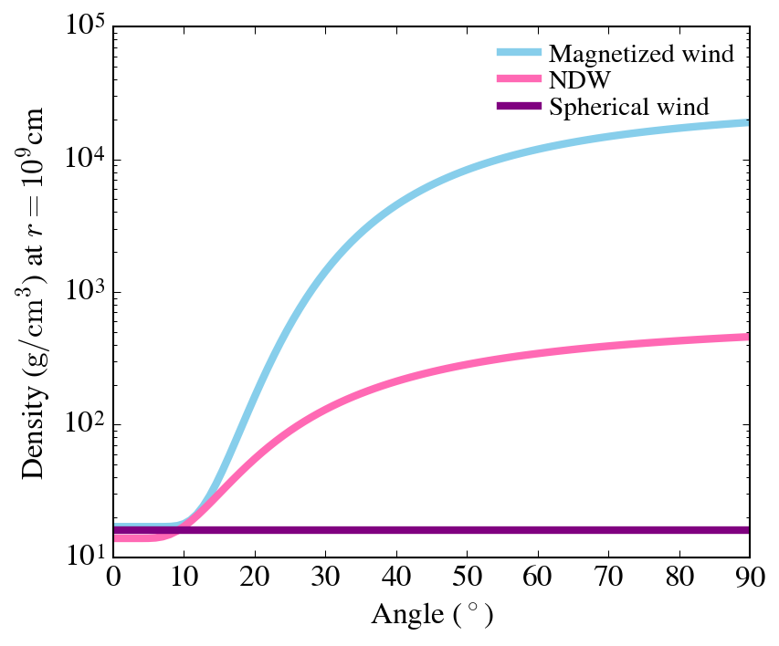
Three different wind prescriptions are simulated, which have different angular structures. The first is a constant uniform spherical wind (Murguia-Berthier et al. 2014). The second is a non-spherical latitudinal distribution in density and velocity (Murguia-Berthier et al. 2017b), whose distribution is based on the global simulations of Perego et al. 2014, accurately representing the neutrino-driven wind from the merger remnant. Additionally, we have included a density profile of a magnetized wind outflow based on the simulations by Janiuk 2019, where the author performs general relativistic magneto-hydrodynamical simulations33 3 We note that although the calculations of Janiuk 2019 were performed for a 3 BH surrounded by 0.1 accretion disk, the resultant angular profiles are very similar to those by Siegel et al. 2014 for a merger remnant. These wind profiles have the advantage that they have been calculated over many more dynamical times, due to the relative numerical simplicity, and thus better resemble a steady state wind solution.. The density profiles in both cases are similar, they are denser in the equator and progressively lighter in the polar region. The density as a function of angle is obtained by averaging the latitudinal profiles at the end of the simulations (Perego et al. 2014; Janiuk 2019). The density of the wind is given by
| (1) |
where is the mass loss rate, is the radial coordinate, is the angular component, and is the velocity of the wind, which is assumed to be constant. For comparison, we plot the angular distributions of density in the three different winds in Figure 1. The ratio of the density in the polar region () and the equator () is for the NDW and for the magnetized outflow. We use two different global values for the mass loss rate, as prescribed in the polar region: /s and /s. This range is motivated by the range of values seen in magnetically-driven and neutrino driven wind calculations (Perego et al. 2014; Siegel et al. 2014; Shibata et al. 2017; Fujibayashi et al. 2018; Nathanail et al. 2019; Geng et al. 2019).

II.3 Evolution of the jet
Initially, the jet is unable to move the wind material at a speed comparable to its own and thus is decelerated. As the jet propagates in the wind a bow shock runs ahead of it, which both heats material and causes it to expand sideways (Ramirez-Ruiz et al. 2002; Bromberg et al. 2011; Salafia et al. 2020). The parameter that controls the evolution of the jet interacting with the wind is (Bromberg et al. 2011; Murguia-Berthier et al. 2017b):
| (2) |
where is the density, is the enthalpy, is the Lorentz factor and the subscripts , refer to the jet and the wind, respectively. At a given time, the jet will have evacuated a channel out to some location where it impinges on the pre-collapse wind, at a working surface advancing at velocity . We balance the momentum fluxes at the working surface to obtain (Begelman & Cioffi 1989; Bromberg et al. 2011; Murguia-Berthier et al. 2017b)
| (3) |
where is the initial velocity of the jet, as determined by . During propagation in the wind, the head of the jet will initially expand at a constant velocity. This is because is independent of , so that remains unchanged (Equation 2). This can be seen in the expansion of the head of the jet during the first s (shown in the bottom panel of Figure 2), which expands at a constant velocity. The surplus energy during this time is deposited within a cocoon surrounding the jet. As the pressure of the cocoon cavity increases, a recollimation shock is formed which minimizes the cross-sectional area of the jet (Figure 2). In this region, depends on the pressure build up within the cocoon region (Bromberg et al. 2011, ;)
| (4) |
This transition is clearly seen after s in the evolution of the jet’s head plotted in Figure 2.
In order for the jet to be successful, the central engine needs to remain active when the jet breaks out of the wind. By considering the time at which the head of the jet reaches the outer edge of the wind, the condition for a successful SGRB jet can be written as:
| (5) |
where . This condition is clearly satisfied in the simulation shown in Figure 2. At the time the jet head breaks out from the wind (s), we required , which is clearly satisfied and the jet remains active. In Section II.4 we investigate the applicability of condition 5 for both spherical and non-spherical winds.
II.4 Winds, jet dynamics and successful jets
The shocks responsible for producing a sGRB must arise after the relativistic jet has broken free from the pre-collapse wind. The majority of compact mergers, with the exception of those involving a black hole, will not collapse immediately and a dense wind will thus remain to impede the advance of the jet. As stated by the condition 5, a sGRB is likely to be produced if the jet triggered by the post-collapse accretion maintains its power for longer than it takes the jet to reach the edge of the wind. If this is not the case, as shown in the top panel in Figure 3, the jet will be choked. On the other hand, if the jet continues to be active and emerges from the wind, the sudden and drastic density drop at the outer edges allows the jet head to accelerate to velocities close to the speed of light44 4 In the case depicted in the bottom panel of Figure 2, the final Lorentz factor is approximately , which is 90% of the initial Lorentz factor., as illustrated in the middle and bottom panels in Figure 3. In the middle panel , while in the bottom panel .


The condition can be used to derive the critical power needed for a jet to be successful, as argued by Murguia-Berthier et al. 2017b. This critical luminosity estimate is shown in Figure 4 in the context of our jet simulations with varying and expanding in a medium with /s. The dots in Figure 4 correspond to successful jets and the crosses are choked jets. As expected, the ratio is critical in determining successful breakout of the expanding jet.

The critical condition for the minimum jet power in Figure 4 has been derived assuming that is constant. This is generally a valid assumption when the jet expands in a wind medium and experiences little recollimation. The applicability of this approximation can be seen by contrasting the evolution of the two jets depicted in the bottom panel in Figure 4. One of them (solid line) experiences significant recollimation before reaching the edge of the jet, while the other one (dashed line) escapes before the cocoon pressure is able to significantly alter the jet’s initial structure. We note that although both jets are successful, the condition plotted in the top panel of Figure 4 places the simulation with (solid line in the bottom panel) below the line. In this case, recollimation permits the jet to expand at a faster rate than the one predicted using the constant assumption. We thus caution the reader that such a constraint should be used as a conservative limit for the necessary jet power.
Additionally, the general formalism used to derive condition given by Eq. 5 makes use of spherical symmetry and as such its applicability is less rigorous when the jet expansion takes place within a non-spherical mass distribution. Figure 5 compares the evolution of two identical jets propagating in two different wind environments. The density profiles in both cases are similar in the polar region but NDW’s profile is progressively denser as it approaches the equatorial region (Figure 1). When the jet propagates in the NDW, the cocoon region is significantly more confined due to the increase in the surrounding pressure. As a result, recollimation occurs earlier in the jet’s propagation when compared to the spherical case and causes the jet to propagate at a faster speed. It is thus important to note that in the realistic wind cases considered in this paper, condition given by Eq. 5 provides a rather robust limit for the minimum luminosity require to produce a successful jet.
As demonstrated here, two dimensional simulations have uncovered some dynamical properties of relativistic flows unanticipated by analytical models, but we caution that there are still some key questions that they cannot tackle. A feature of the jet-wind interaction is that there will surely be some mass entertainment and maybe more importantly, there can be an exchange of linear momentum with the surrounding material. Because of this, we cautioned that higher resolution is needed because even a tiny mass fraction of baryons loading down the jet could severely limits the attainable Lorentz factor (here assumed to be only 10 for numerical convenience). Additionally, the symmetry-breaking involved in transitioning from two to three dimensions is crucial for understanding the nonlinear development of instabilities, leading to qualitatively new phenomena (Rossi et al. 2008; Meliani & Keppens 2010; López-Cámara et al. 2013; Gottlieb et al. 2018b; Gottlieb et al. 2018a; Matsumoto & Masada 2019; Gottlieb et al. 2020b). Another topic which seems ripe for a more sophisticated treatment concerns the possibility that the initial jet is a magnetically confined configuration, whose collimation properties are not as drastically modified by the distribution of the external material (Mizuno et al. 2012; Bromberg & Tchekhovskoy 2016; Tchekhovskoy & Bromberg 2016; Geng et al. 2019; Nathanail et al. 2020b; Gottlieb et al. 2020a; Nathanail et al. 2020a; Mukherjee et al. 2020).


II.5 Jet structure
We perform different simulations, for a given wind profile, by altering the lifetime of the wind (), which is directly related to the time it takes the merger remnant to collapse to a black hole. We also changed the duration of the jet (), which is the characteristic time the central engine is active and is broadly related to the duration of the event. We show our results in Figures 6, 7 and 8, where we plot the density and Lorentz factor distributions of jets propagating through a spherical wind, a neutrino-driven wind and a magnetically ejected wind, respectively. The energy per unit solid angle at the end of the simulation is estimated as in Duffell et al. 2015.
The interaction of the jet with the wind will result in an angular redistribution of the jet’s energy, which can naturally give rise to a different afterglow light curve than the one from the original top-hat structure (Lazzati et al. 2017; Duffell et al. 2018; Bromberg et al. 2018; Granot et al. 2018; Lamb & Kobayashi 2018; Kathirgamaraju et al. 2018; van Eerten et al. 2018; Lamb et al. 2019; Salafia et al. 2019; Lazzati et al. 2020; Gottlieb et al. 2020b). In what follows, we explore how the properties of the pre-collapse wind affect the structure of a jet propagating through it.
Common to all calculations is the altering of and . Also shown is the final angular distribution of the energy in the relativistic jet. In all simulations we define the core angle of the jet, after its propagation, as the angle where the Lorentz factor of the jet decreases by a factor of 2 from its initial value. The resulting core angles range from to , which are similar to the values quoted in the literature (Lyman et al. 2018; D’Avanzo et al. 2018; Troja et al. 2018; Salafia et al. 2019; Ghirlanda et al. 2019; Lazzati et al. 2020; Nathanail et al. 2020b). The final angular distribution of Lorentz factor is found to be well represented by a Gaussian distribution. In all cases, the jet, which is originally a top-hat, spreads laterally thus resulting in a structured jet.
In addition to the density of the wind, which depends primarily on the mass loss rate, the ratio has a decisive effect on the appearance of a jet propagating through it. This is because it determines the time the jet resides within the interaction region (as governed by ) which in turn regulates the amount of relativistic material that is shocked. The importance of this ratio can be clearly seen in the Bottom panels of Figures 6, 7 and Figure 8. If the delay time is larger or comparable to the duration of the jet, the time it takes for the jet to break free from the wind is augmented. In this case, the afterglow emission would be dominated by the emission of the laterally spreading relativistic material, which is located at larger angles relative to the rotation axis of the merger remnant. On the other hand, if the jet produced by the accretion onto the black hole maintains its energy for much longer than it takes the jet head to reach the edge of the wind, the core of the relativistic jet would contain substantially more energy than the off-axis material, so that it is likely to dominate the afterglow flux even after expanding for a longer time. The detection of varying afterglow signatures would be a test of the neutron star merger model; and the precise inference of the angular structure of the jet may help constrain the properties of the wind and the lifetime of the merger remnant.
The strength of the baryon loaded wind is also a key parameter. If the mass loss rate is increased to /s in the polar region and the luminosity is kept at erg/s, the wind would choke the jet, rendering the sGRB unsuccessful. The jet, in this environment can become successful if its power is increased, as governed by (Bromberg et al. 2011). In Figure 9, we show the effects of altering the mass loss rate and the luminosity of the wind but leaving . unchanged. As expected, the evolution of the jet remains unchanged and the simulation outputs in these two cases look almost identical.


III Relevance to GW170817
Several groups (Lazzati et al. 2018; Margutti et al. 2018; Lyman et al. 2018; D’Avanzo et al. 2018; Troja et al. 2018; Ghirlanda et al. 2019; Salafia et al. 2019; Lazzati et al. 2020) have studied the origin of the afterglow emission of GW170817 and concluded that it can be explained by invoking a model where the sGRB was successful and the observer lies off axis to the jet. A common feature of all models is the need for significant amount of energy at larger angles, which as we have argued here can be a natural consequence of the interaction of the jet with the pre-collapse wind. In this section we endeavor to compare our simulation results to the jet models constructed for GW170817.
In Figure 10 we plot the range of wind parameters used in our study and compare them with the constraints derived by the presence of the blue kilonova. The blue line represents the limit marked by the total mass derived to produce the blue component of the kilonova (Kasen et al. 2017). We note that the total mass ejected by the wind in our simulations is below this value.
Various groups inferred different energy distributions for the jet. In Figure 11 we compare their best fit models for the jet profiles with those obtained from our simulations. The results from our simulations are in broad agreement with the energy distributions derived from afterglow observations. We thus conclude that the structure of an initially top-hat jet can be modified by its interaction with the pre-collapse wind and, after the jet emerges from this region, can have a structure that closely resembles the one deduced for GW170817. So in these models the -rays would be restricted to a narrow beam, even though outflow with a more moderate Lorentz factor, which is relevant to the afterglow emission, is spread over a wider range of angles.
While the properties of the pre-collapse wind have an important effect on the appearance of a jet propagating through it (Figure 11), our calculations suggest that is the essential parameter that controls how much relativistic energy is distributed at large angles.
Figure 12 illustrates the effect of varying for jets propagating within the three different wind profiles we have considered in this study and the different mass loss rates. It shows how the ratio of the energy contained in the core of the jet to that residing outside it increases as augments. As argued above, we also see that changes in the mass loss rate have a less dramatic effect when compared to variations in .
In the case of a successful break-through, the resultant jet structure could result in an afterglow signature similar to that observed in GW170817 if the time it took for the merger remnant to collapse is similar to the observed duration of the event. An upper limit for can be derived by requiring a successful jet (Murguia-Berthier et al. 2017b). A successful jet can be produced if the central engine remains active for a time longer than the time it takes for the jet to break through the wind:
| (6) |
where , and the subscript referring to the head of the jet. This condition is derived using the evolution of the working surface, where the velocity of the head of the jet is given by Equation 3.
A lower limit for can be found using Figure 12, which shows that in order for our models to explain the afterglow of GW170817, a long interaction with the wind is required. In particular, in order to be in agreement with the most recent afterglow models, we require . At smaller , the core of the jet carries the bulk of the energy and, as such, it would closely resemble a top-hat model which is inconsistent with current observations. Models that have more extended wings carrying a larger amount of energy thus require longer interaction times between the jet and the wind. Using s (Goldstein et al. 2017), we derive the following stringent limit .
The constraint given above can be combined with the successful sGRB requirement given by Equation 6 in order to derive a range of permitted values for . Making use of the broad range of values derived for GW170817, in Figure 13 we show the allowed (pink) region for as a function . The lower limit, which is independent of , is derived from the requirement that , as seen in Fig 12.The upper limit, on the other hand, is derived using equation 6 with the additional constraint that as motivated by the range of realistic values seen in merger calculations (Siegel et al. 2014; Fujibayashi et al. 2018; Nathanail et al. 2019; Perego et al. 2014). A strict upper limit for the time of collapse can be obtained by taking into account the time delay between the GW and the -ray signal, which has been observed to be around s (Abbott et al. 2017a; Goldstein et al. 2017). The three constraints can then be combined to derive a range of permitted values for s.

This finding gives further credence to the idea that in the case of GW170817, the collapse into a black hole was indeed delayed. Yet this argument comes from a completely different line of reasoning than those given in the literature:
- •
Granot et al. 2017 set a constraint of s based on the expected lifetime of a hyper-massive NS.
- •
Gottlieb et al. 2018b find s based on the time of the shock breakout compared to the observed delay between gravitational waves and the -rays.
- •
Nakar et al. 2018 perform simulations of a mildly relativistic cocoon using a time delay of s which is able to reproduce the observed data.
- •
Gottlieb et al. 2018b perform simulations of a cocoon shock breakout and they can reproduce the observed afterglow emission with s.
- •
Metzger et al. 2018 set a constraint of s based on the amount of blue ejecta expected from a magnetized wind.
- •
Xie et al. 2018 perform numerical simulations and show that a delay time of s is able to reproduce the afterglow data
- •
Gill et al. 2019b did a comprehensive analysis and estimated the collapse time to be s. They combined several constraints including the delay time between the gravitational wave and electromagnetic signal, a comparison on the observational mass of the blue ejecta and constraints based on a successful jet.
- •
van Putten et al. 2019 obtain a limit of s based on observations of extended emission.
- •
Lazzati et al. 2020 favour the delay time to be around s by parameter space exploration of jet-wind interactions using an analytical formalism.
- •
Hamidani et al. 2020 analytically estimate a delay time of s which they compared to detailed numerical calculations.
Our estimate for , which is based on the angular structure of a successful jet as inferred from afterglow observations, is roughly consistent with these various estimates.
Many binary neutron star mergers are thought to produce sGRBs when collapsing to black holes but some merger remnants may experience significant delays before collapsing. One expects various outcomes ranging from sGRBs with narrow beams from prompt collapse to structured jets with bright and weak sGRBs for longer collapse timescales. The properties of the afterglow signatures produced by successful and non-successful jets would provide a natural test to distinguish between these different progenitor avenues. The different jet structure can be used to obtain the different afterglow emission (De Colle et al. 2012b; De Colle et al. 2018; Urrutia et al. 2020).
References
- Abbott et al. (2017a) Abbott, B. P., Abbott, R., Abbott, T. D., et al. 2017a, Physical Review Letters, 119, 161101
- Abbott et al. (2017b) —. 2017b, ApJ, 848, L12
- Aloy et al. (2005) Aloy, M. A., Janka, H.-T., & Müller, E. 2005, A&A, 436, 273
- Baiotti et al. (2008) Baiotti, L., Giacomazzo, B., & Rezzolla, L. 2008, Phys. Rev. D, 78, 084033
- Begelman & Cioffi (1989) Begelman, M. C., & Cioffi, D. F. 1989, ApJ, 345, L21
- Beniamini et al. (2020) Beniamini, P., Granot, J., & Gill, R. 2020, MNRAS, 493, 3521
- Bromberg et al. (2011) Bromberg, O., Nakar, E., Piran, T., & Sari, R. 2011, ApJ, 740, 100
- Bromberg & Tchekhovskoy (2016) Bromberg, O., & Tchekhovskoy, A. 2016, MNRAS, 456, 1739
- Bromberg et al. (2018) Bromberg, O., Tchekhovskoy, A., Gottlieb, O., Nakar, E., & Piran, T. 2018, MNRAS, 475, 2971
- Ciolfi (2020) Ciolfi, R. 2020, MNRAS, 495, L66
- Ciolfi et al. (2017) Ciolfi, R., Kastaun, W., Giacomazzo, B., et al. 2017, Phys. Rev. D, 95, 063016
- Ciolfi et al. (2019) Ciolfi, R., Kastaun, W., Kalinani, J. V., & Giacomazzo, B. 2019, Phys. Rev. D, 100, 023005
- Coulter et al. (2017) Coulter, D. A., Foley, R. J., Kilpatrick, C. D., et al. 2017, Science, 358, 1556
- D’Avanzo et al. (2018) D’Avanzo, P., Campana, S., Salafia, O. S., et al. 2018, A&A, 613, L1
- De Colle et al. (2012a) De Colle, F., Granot, J., López-Cámara, D., & Ramirez-Ruiz, E. 2012a, ApJ, 746, 122
- De Colle et al. (2018) De Colle, F., Lu, W., Kumar, P., Ramirez-Ruiz, E., & Smoot, G. 2018, MNRAS, 478, 4553
- De Colle et al. (2012b) De Colle, F., Ramirez-Ruiz, E., Granot, J., & Lopez-Camara, D. 2012b, ApJ, 751, 57
- Dessart et al. (2009) Dessart, L., Ott, C. D., Burrows, A., Rosswog, S., & Livne, E. 2009, ApJ, 690, 1681
- Duffell et al. (2018) Duffell, P. C., Quataert, E., Kasen, D., & Klion, H. 2018, ApJ, 866, 3
- Duffell et al. (2015) Duffell, P. C., Quataert, E., & MacFadyen, A. I. 2015, ApJ, 813, 64
- Eichler et al. (1989) Eichler, D., Livio, M., Piran, T., & Schramm, D. N. 1989, Nature, 340, 126
- Fujibayashi et al. (2018) Fujibayashi, S., Kiuchi, K., Nishimura, N., Sekiguchi, Y., & Shibata, M. 2018, ApJ, 860, 64
- Geng et al. (2019) Geng, J.-J., Zhang, B., Kölligan, A., Kuiper, R., & Huang, Y.-F. 2019, ApJ, 877, L40
- Ghirlanda et al. (2019) Ghirlanda, G., Salafia, O. S., Paragi, Z., et al. 2019, Science, 363, 968
- Gill et al. (2019a) Gill, R., Granot, J., De Colle, F., & Urrutia, G. 2019a, ApJ, 883, 15
- Gill et al. (2019b) Gill, R., Nathanail, A., & Rezzolla, L. 2019b, ApJ, 876, 139
- Goldstein et al. (2017) Goldstein, A., Veres, P., Burns, E., et al. 2017, ApJ, 848, L14
- Gottlieb et al. (2020a) Gottlieb, O., Bromberg, O., Singh, C. B., & Nakar, E. 2020a, arXiv e-prints, arXiv:2007.11590
- Gottlieb et al. (2020b) Gottlieb, O., Nakar, E., & Bromberg, O. 2020b, arXiv e-prints, arXiv:2006.02466
- Gottlieb et al. (2018a) Gottlieb, O., Nakar, E., & Piran, T. 2018a, MNRAS, 473, 576
- Gottlieb et al. (2018b) Gottlieb, O., Nakar, E., Piran, T., & Hotokezaka, K. 2018b, MNRAS, 479, 588
- Granot et al. (2018) Granot, J., Gill, R., Guetta, D., & De Colle, F. 2018, MNRAS, 481, 1597
- Granot et al. (2017) Granot, J., Guetta, D., & Gill, R. 2017, ApJ, 850, L24
- Hamidani & Ioka (2020) Hamidani, H., & Ioka, K. 2020, arXiv e-prints, arXiv:2007.10690
- Hamidani et al. (2020) Hamidani, H., Kiuchi, K., & Ioka, K. 2020, MNRAS, 491, 3192
- Janiuk (2019) Janiuk, A. 2019, ApJ, 882, 163
- Kasen et al. (2017) Kasen, D., Metzger, B., Barnes, J., Quataert, E., & Ramirez-Ruiz, E. 2017, Nature, 551, 80
- Kathirgamaraju et al. (2018) Kathirgamaraju, A., Barniol Duran, R., & Giannios, D. 2018, MNRAS, 473, L121
- Kathirgamaraju et al. (2019) Kathirgamaraju, A., Tchekhovskoy, A., Giannios, D., & Barniol Duran, R. 2019, MNRAS, 484, L98
- Lamb & Kobayashi (2018) Lamb, G. P., & Kobayashi, S. 2018, MNRAS, 478, 733
- Lamb et al. (2018) Lamb, G. P., Mandel, I., & Resmi, L. 2018, MNRAS, 481, 2581
- Lamb et al. (2019) Lamb, G. P., Lyman, J. D., Levan, A. J., et al. 2019, ApJ, 870, L15
- Lazzati et al. (2020) Lazzati, D., Ciolfi, R., & Perna, R. 2020, ApJ, 898, 59
- Lazzati et al. (2017) Lazzati, D., Deich, A., Morsony, B. J., & Workman, J. C. 2017, MNRAS, 471, 1652
- Lazzati & Perna (2019) Lazzati, D., & Perna, R. 2019, arXiv e-prints, arXiv:1904.08425
- Lazzati et al. (2018) Lazzati, D., Perna, R., Morsony, B. J., et al. 2018, Physical Review Letters, 120, 241103
- Lee & Ramirez-Ruiz (2007) Lee, W. H., & Ramirez-Ruiz, E. 2007, New Journal of Physics, 9, 17
- Lee et al. (2005) Lee, W. H., Ramirez-Ruiz, E., & Granot, J. 2005, ApJ, 630, L165
- Lee et al. (2009) Lee, W. H., Ramirez-Ruiz, E., & López-Cámara, D. 2009, ApJ, 699, L93
- López-Cámara et al. (2013) López-Cámara, D., Morsony, B. J., Begelman, M. C., & Lazzati, D. 2013, ApJ, 767, 19
- Lyman et al. (2018) Lyman, J. D., Lamb, G. P., Levan, A. J., et al. 2018, Nature Astronomy, 2, 751
- Margutti et al. (2018) Margutti, R., Alexander, K. D., Xie, X., et al. 2018, ApJ, 856, L18
- Matsumoto & Masada (2019) Matsumoto, J., & Masada, Y. 2019, MNRAS, 490, 4271
- McKinney et al. (2012) McKinney, J. C., Tchekhovskoy, A., & Blandford, R. D. 2012, MNRAS, 423, 3083
- McKinney et al. (2014) McKinney, J. C., Tchekhovskoy, A., Sadowski, A., & Narayan, R. 2014, MNRAS, 441, 3177
- Meliani & Keppens (2010) Meliani, Z., & Keppens, R. 2010, A&A, 520, L3
- Metzger et al. (2018) Metzger, B. D., Thompson, T. A., & Quataert, E. 2018, ApJ, 856, 101
- Mizuno et al. (2012) Mizuno, Y., Lyubarsky, Y., Nishikawa, K.-I., & Hardee, P. E. 2012, ApJ, 757, 16
- Mooley et al. (2018a) Mooley, K. P., Frail, D. A., Dobie, D., et al. 2018a, ApJ, 868, L11
- Mooley et al. (2018b) Mooley, K. P., Deller, A. T., Gottlieb, O., et al. 2018b, Nature, 561, 355
- Mösta et al. (2020) Mösta, P., Radice, D., Haas, R., Schnetter, E., & Bernuzzi, S. 2020, arXiv e-prints, arXiv:2003.06043
- Mukherjee et al. (2020) Mukherjee, D., Bodo, G., Mignone, A., Rossi, P., & Vaidya, B. 2020, arXiv e-prints, arXiv:2009.10475
- Murguia-Berthier et al. (2014) Murguia-Berthier, A., Montes, G., Ramirez-Ruiz, E., De Colle, F., & Lee, W. H. 2014, ApJ, 788, L8
- Murguia-Berthier et al. (2017a) Murguia-Berthier, A., Ramirez-Ruiz, E., Kilpatrick, C. D., et al. 2017a, ApJ, 848, L34
- Murguia-Berthier et al. (2017b) Murguia-Berthier, A., Ramirez-Ruiz, E., Montes, G., et al. 2017b, ApJ, 835, L34
- Nagakura et al. (2014) Nagakura, H., Hotokezaka, K., Sekiguchi, Y., Shibata, M., & Ioka, K. 2014, ApJ, 784, L28
- Nakar et al. (2018) Nakar, E., Gottlieb, O., Piran, T., Kasliwal, M. M., & Hallinan, G. 2018, ApJ, 867, 18
- Nakar & Piran (2020) Nakar, E., & Piran, T. 2020, arXiv e-prints, arXiv:2005.01754
- Narayan et al. (1992) Narayan, R., Paczynski, B., & Piran, T. 1992, ApJ, 395, L83
- Nathanail et al. (2020a) Nathanail, A., Gill, R., Porth, O., Fromm, C. M., & Rezzolla, L. 2020a, arXiv e-prints, arXiv:2009.09714
- Nathanail et al. (2020b) —. 2020b, MNRAS, 495, 3780
- Nathanail et al. (2019) Nathanail, A., Porth, O., & Rezzolla, L. 2019, ApJ, 870, L20
- Nedora et al. (2020) Nedora, V., Bernuzzi, S., Radice, D., et al. 2020, arXiv e-prints, arXiv:2008.04333
- Perego et al. (2014) Perego, A., Rosswog, S., Cabezón, R. M., et al. 2014, MNRAS, 443, 3134
- Qian et al. (2018) Qian, Q., Fendt, C., & Vourellis, C. 2018, ApJ, 859, 28
- Ramirez-Ruiz et al. (2019) Ramirez-Ruiz, E., Andrews, J. J., & Schrøder, S. L. 2019, ApJ, 883, L6
- Ramirez-Ruiz et al. (2002) Ramirez-Ruiz, E., Celotti, A., & Rees, M. J. 2002, MNRAS, 337, 1349
- Rezzolla et al. (2011) Rezzolla, L., Giacomazzo, B., Baiotti, L., et al. 2011, ApJ, 732, L6
- Rossi et al. (2008) Rossi, P., Mignone, A., Bodo, G., Massaglia, S., & Ferrari, A. 2008, A&A, 488, 795
- Rosswog & Ramirez-Ruiz (2002) Rosswog, S., & Ramirez-Ruiz, E. 2002, MNRAS, 336, L7
- Rosswog & Ramirez-Ruiz (2003) —. 2003, MNRAS, 343, L36
- Rosswog et al. (2003) Rosswog, S., Ramirez-Ruiz, E., & Davies, M. B. 2003, MNRAS, 345, 1077
- Ruiz et al. (2016) Ruiz, M., Lang, R. N., Paschalidis, V., & Shapiro, S. L. 2016, ApJ, 824, L6
- Ruiz et al. (2019) Ruiz, M., Tsokaros, A., Paschalidis, V., & Shapiro, S. L. 2019, Phys. Rev. D, 99, 084032
- Ryan et al. (2020) Ryan, G., van Eerten, H., Piro, L., & Troja, E. 2020, ApJ, 896, 166
- Salafia et al. (2020) Salafia, O. S., Barbieri, C., Ascenzi, S., & Toffano, M. 2020, A&A, 636, A105
- Salafia et al. (2019) Salafia, O. S., Ghirlanda, G., Ascenzi, S., & Ghisellini, G. 2019, A&A, 628, A18
- Sa̧dowski et al. (2015) Sa̧dowski, A., Narayan, R., Tchekhovskoy, A., et al. 2015, MNRAS, 447, 49
- Shibata et al. (2017) Shibata, M., Kiuchi, K., & Sekiguchi, Y.-i. 2017, Phys. Rev. D, 95, 083005
- Siegel et al. (2014) Siegel, D. M., Ciolfi, R., & Rezzolla, L. 2014, ApJ, 785, L6
- Tchekhovskoy & Bromberg (2016) Tchekhovskoy, A., & Bromberg, O. 2016, MNRAS, 461, L46
- Troja et al. (2018) Troja, E., Piro, L., Ryan, G., et al. 2018, MNRAS, 478, L18
- Turk et al. (2011) Turk, M. J., Smith, B. D., Oishi, J. S., et al. 2011, ApJS, 192, 9
- Urrutia et al. (2020) Urrutia, G., De Colle, F., Murguia-Berthier, A., & Ramirez-Ruiz, E. 2020, arXiv e-prints, arXiv:2011.06729
- van Eerten et al. (2018) van Eerten, E. T. H., Ryan, G., Ricci, R., et al. 2018, arXiv e-prints, arXiv:1808.06617
- van Putten et al. (2019) van Putten, M. H. P. M., Della Valle, M., & Levinson, A. 2019, ApJ, 876, L2
- Wu & MacFadyen (2018) Wu, Y., & MacFadyen, A. 2018, ApJ, 869, 55
- Xie et al. (2018) Xie, X., Zrake, J., & MacFadyen, A. 2018, ApJ, 863, 58