Multi-Frequency General Relativistic Radiation-Hydrodynamics with Closure
Abstract
We report on recent upgrades to our general relativistic radiation-magnetohydrodynamics code, Cosmos++, which expands the two-moment, , radiation treatment from grey to multi-frequency transport, including Doppler and gravitational frequency shifts. The solver accommodates either photon (Bose-Einstein) or neutrino (Fermi-Dirac) statistical distribution functions with absorption, emission, and elastic scattering processes. An implicit scheme is implemented to simultaneously solve the primitive inversion problem together with the radiation-matter coupling source terms, providing stability over a broad range of opacities and optical depths where the interactions terms can be stiff. We discuss our formulations and numerical methods, and validate our methods against a wide variety of test problems spanning optically thin to thick regimes in flat, weakly curved, and strongly curved spacetimes.
Keywords:
Computational methods — Radiative magnetohydrodynamicsI Introduction
Today we are part of an exciting multi-messenger era in astronomy. Telescopes cover the entire electromagnetic (EM) spectrum, with nightly full-sky coverage becoming a reality (Chambers et al. 2016; Ivezić et al. 2019; Graham et al. 2019, e.g.,). Additionally, cosmic ray detectors (Cherenkov Telescope Array Consortium et al. 2019, e.g.,), neutrino detectors (Aartsen et al. 2019, e.g.,), and now gravitational wave detectors (Abbot et al. 2018) give us views of the universe beyond EM radiation, and as each new means of observation has been added, new discoveries have quickly followed (Abbot et al. 2017; Metzger 2017; IceCube Collaboration et al. 2018; Keivani et al. 2018; Fang et al. 2019, e.g.,). Certainly many more are to be expected.
A principle focus of multi-messenger astronomy is the transient universe (Charles & Shaw 2013), particularly events that are characterized by short bursts of electromagnetic radiation, possibly accompanied by cosmic ray, neutrino, or gravitational wave signals, such as kilonovae (Abbot et al. 2017; Metzger 2017, e.g.,), fast radio bursts (Burke-Spolaor 2018; Wang et al. 2020, e.g.,), gamma ray bursts (Burns et al. 2019, e.g.,), and tidal disruption events (Senno et al. 2017, e.g.,). These events are often highly energetic and commonly associated with compact objects (white dwarfs, neutron stars, or black holes), suggesting relativistic physics plays a role.
The many new discoveries in multi-messenger astronomy need to be matched by corresponding developments in the computational tools that help in their interpretation and understanding. Over the decades, advances in observational capabilities have seen parallel developments in astrophysical simulation tools toward ever higher levels of sophistication, starting from relatively simple hydrodynamic and N-body simulations to magnetohydrodynamics (MHD), radiation MHD, and beyond (see Abramowicz & Fragile 2013, for a review of relativistic code development). Most transient phenomena require some combination of relativity, hydrodynamics, magnetic fields, and radiation to be adequately modeled. Fortunately, the number of codes available for advanced radiation MHD simulations has quite literally exploded in recent years (Farris et al. 2008; Müller et al. 2010; Shibata et al. 2011; Zanotti et al. 2011; Jiang et al. 2012; Lentz et al. 2012; Sa̧dowski et al. 2013; Zhang et al. 2013; González et al. 2015; Just et al. 2015; Tominaga et al. 2015; Kuroda et al. 2016; Skinner et al. 2019; Ryan & Dolence 2020; Weih et al. 2020, an incomplete list includes). Our own contribution is the general relativistic radiation magnetohydrodynamics code, Cosmos++ (Anninos et al. 2005; Fragile et al. 2012; Fragile et al. 2014), which includes a discontinuous-Galerkin variant, CosmosDG (Anninos et al. 2017).
As ever, though, numerical simulations are only an approximation to reality. The current limitation in radiation MHD is that solving the full Boltzmann transport equation remains computationally challenging and not entirely practical in most scenarios, owing to the large number of degrees of freedom (in space and frequency) and wide range of optical depths, although new formulations have been developed for this purpose (Davis & Gammie 2020). Therefore, most codes today treat some simplified form of radiation. One common approach is to use a scheme where only the first few moments of the radiation distribution function are evolved (Thorne 1981; Shibata et al. 2011). The most basic is the flux-limited diffusion approximation (Levermore & Pomraning 1981; Pomraning 1981), which only treats the zeroth moment, meaning it retains information only about the radiation intensity, but not the direction of its propagation. A two-moment scheme, such as (Levermore 1984; Dubroca & Feugeas 1999; González et al. 2007), retains both the intensity and (average) direction of radiation flow, yet still closes the system of equations at a level that remains computationally reasonable. This approach has seen wide implementation in the context of black-hole accretion (Sa̧dowski et al. 2013; Fragile et al. 2014; McKinney et al. 2014; Mishra et al. 2016; Takahashi et al. 2016; Fragile et al. 2018b), black-hole–neutron-star mergers (Foucart et al. 2015; Foucart et al. 2016a), binary neutron stars (Foucart et al. 2016b; Sekiguchi et al. 2016), core-collapse supernovae (O’Connor 2015; Just et al. 2015; Kuroda et al. 2016), and the interaction of Type I X-ray bursts with accretion disks (Fragile et al. 2018a; Fragile et al. 2020).
Another simplification is that most relativistic radiation MHD codes today assume a frequency-integrated (or grey) opacity and evolve the radiation field with a single characteristic frequency. However, resolving the photon (or neutrino) frequency (energy), even crudely, can be crucially important to properly modeling and understanding many transient phenomena, such as core-collapse supernovae (Janka 2012; Burrows 2013; Foglizzo et al. 2015, e.g.,), tidal disruption events (Dai et al. 2018), and the outbursts of black hole X-ray binaries.
This is the goal of our current work, to extend our radiation transport capabilities from a frequency-integrated (grey) approximation to a multi-frequency (equivalently multi-energy or sometimes called multi-group) method by discretizing the radiation energy and flux equations in frequency as well as space and time. As in our previous paper (Fragile et al. 2014), we adopt the closure for general relativistic transport, though we have additionally developed a multi-frequency, flux-limited diffusion (with an anisotropic Eddington tensor) solver for Newtonian systems. Much of the methodology, including the formalism and numerical methods, discussed in this paper is taken from Fragile et al. 2014, and we occasionally refer the reader back to that paper for further details, particularly regarding the high resolution shock capturing algorithms and the primitive inversion scheme. All of those specifics are similar to what we have developed for this work, except they are applied to the radiation fields in each frequency bin separately. The primitive inversion scheme utilizes a first-order Taylor expansion of the conserved fields together with the radiation coupling terms, again similar to our previous work except here the dimension of the matrix system scales with the number of radiation bins, and the coupling to the hydrodynamics occurs after integrating each source contribution over frequency. The most significant new element that comes from frequency-dependent transport is the introduction of a source term responsible for advecting energies in frequency space as radiation propagates through gravitational fields or experiences fluid velocities that produce shifts in the photon frequencies (or neutrino energies).
As for the organization of this paper, Section II follows with an overview of the essential formalism and conservation equations. Section III discusses our numerical implementation with an emphasis on the new elements: frequency advection, closure relations, and the implicit approach for solving the coupled primitive inversion and multi-frequency radiation source terms. Section IV reports on a series of validating test problems, and we conclude in Section V.
Most of the equations in this paper are written in units where , although in a few places we leave in factors of for clarity. We adopt the usual convention whereby Greek (Latin) indices refer to spacetime (spatial) coordinates and adopt a metric signature.
II Formalism
A multi-frequency treatment of radiation transport can be derived by selecting a finite set of frequency groups (or bins) and defining the discrete energy densities as integrals of the energy spectral densities, , over the group frequency interval . Mathematically, , and therefore , where and are the lower and upper limits to our frequency bins. In this notation, the total stress-energy tensor can be written
| (1) |
where is the fluid component, and is the spectral radiation stress tensor summed over all radiation components representing photons or different neutrino species. For this work we consider only single species (either photon or single flavor neutrino) transport.
The spectral radiation tensor, , can be written in any number of ways, depending on the frame of reference. For example, the following representations
| (2) | |||||
| (3) | |||||
| (4) |
are commonly used for Eulerian (lab), co-moving (fluid), or isotropic (radiation) frame formalisms, respectively, where is a timelike vector orthogonal to the spacelike hypersurface, is the fluid rest frame 4-velocity, and is the lapse function. The quantities , , and represent the frequency-dependent radiation energy densities in the different frames; likewise, and represent the radiation momentum densities. Finally, and are most often referred to as the pressure or stress tensors of the radiation. In previous work (Fragile et al. 2014), we adopted the radiation frame formalism (Sa̧dowski et al. 2013), which offers some unique advantages for computation. Notice, for example, that the radiation pressure does not appear in the isotropic stress-tensor, as it implicitly represents the covariant formulation of the closure scheme (Levermore 1984), which assumes the radiation is isotropic in the radiation rest frame11 1 We are as yet unaware of any general proof of the existence of such a frame, though from our experience we have not found any cases where this formulation breaks down.. There is also no explicit appearance of a radiation momentum density in the radiation frame. However, certain calculations are most conveniently done in either of the fluid or Eulerian frames, so we retain the flexibility to transform between the different reference frames and fields. To this end, we explicitly write out here some of the more important relations between radiation fields and moments.
First, the frame-dependent primitive moments are extracted from the spectral radiation stress-tensor (or equivalently the conserved or evolved radiation fields) as
| (5) |
and
| (6) |
where is the spatial metric, is the fluid-frame projection metric, and the second rank tensors and are determined by closure relations to be discussed later. Additionally we can relate the energy and flux variables directly via (Shibata et al. 2011)
| (7) | |||||
| (8) |
where is the Lorentz factor. The Eulerian frame flux vector and pressure tensor additionally satisfy , implying , a fact we have exploited in writing Equations (7) and (8).
The radiation variables, and , representing the spectral radiation energy density in the radiation rest frame and the 4-velocity of the radiation rest frame itself, can easily be defined in terms of either lab or fluid frame tensor components. In particular, the following quadratic equations
| (9) | |||||
| (10) |
can be solved for and (Sa̧dowski et al. 2013). The remaining spatial components of the radiation 4-velocity, , are derived from the time components of the radiation stress-tensor.
Following the truncated moment formalism (Thorne 1981; Shibata et al. 2011), the radiation conservation equations become
| (11) |
where represents radiation-matter interaction source terms, and is the third-rank moment tensor associated with Doppler and gravitational frequency shifts.
These radiation equations are solved together with the conservation equations for mass and fluid stress-energy . Ignoring non-ideal effects and magnetic fields, the fluid stress-energy tensor takes the form
| (12) |
where is the gas pressure. Although we do not consider magnetic fields or viscosity in this work, we advertise that both of these physics capabilities are currently fully integrated with this multi-frequency radiation upgrade. We refer the reader to Fragile et al. 2012 and Fragile et al. 2018b for details on their respective implementations.
Coupling of the fluid and radiation equations occurs through the radiation 4-force density, , written in the form
| (13) |
where and represent the frequency-dependent absorption/emission and elastic scattering opacities, respectively; is the Bose-Einstein or Fermi-Dirac statistical distribution function
| (14) |
where is the chemical potential, (1) is the statistical weight for photons (neutrinos), and (-1) for photons (neutrinos). The grey (frequency integrated) version of equation (13) can be written
| (15) |
where is the radiation constant (different for photons and neutrinos) and , , and are the flux, absorption, and Planck mean opacities, respectively.
Expanding out the covariant derivatives, the full set of conservation equations to be solved are written as
| (16) |
| (17) |
| (18) |
| (19) |
| (20) |
where , is the rest-frame fluid density, is the relativistic boost factor, is the fluid transport velocity, is the 4-metric determinant, is the geometric connection coefficients of the metric, is the total energy density, is the covariant momentum density, is the conserved radiation spectral energy, is the conserved radiation spectral momentum, and .
III Numerical Implementation
Equations (16) - (20) are solved by operator splitting terms into spacetime advection, curvature, frequency advection, and radiation-matter coupling. The first three contributions are solved using high-order explicit methods, while the fourth is updated with a fully implicit approach, which provides stability when radiation-matter interactions become stiff relative to a hydrodynamic time scale, as they often do when strongly coupled. Solution methods for each of these contributions are discussed below.
III.1 Advection and Curvature
The radiation conservation laws (19) - (20) are identical in form to the fluid energy and momentum conservation equations already solved in Cosmos++, and are amenable to similar numerical techniques, specifically the high-resolution shock-capturing (HRSC) scheme as described in Fragile et al. 2012.
Representing conserved fields as , the discrete finite volume representation of equations (16) - (20) are written in generic fashion as
| (21) |
where contains the curvature source terms, are the fluxes, and represents the intermediate solution state (accounting for advection and curvature, but not frequency shift or coupling terms). Notice that both the flux and curvature source terms are computed from the set of primitive, not conserved, fields.
One of the differences between this work and that presented in Fragile et al. 2014 is the choice of primitive fields. Here we have opted to use the fluid and spectral radiation 4-velocities [ and ] and not the normal observer projected 4-velocities () that we used previously. With this change, the set of primitive variables becomes , where is the specific internal energy as measured in the fluid rest frame.
The flux terms are calculated at zone faces using either the Harten-Lax-van Leer (HLL) or Lax-Friedrichs (LF) Riemann solver with options for linear or PPM slope limited reconstruction of the primitive fields. For the HLL solver this takes the form
| (22) |
where R (L) subscripts denote right (left) reconstructed states, and () is the characteristic maximum (minimum) wave speed.
One of the advantages of formulating radiation transport in terms of the primitive radiation variables, and , is that it simplifies the calculation of characteristic radiation wave speeds required for the Riemann solvers. We generally follow the prescription outlined in our grey treatment (Fragile et al. 2012) where we effectively replace the fluid velocity with the radiation velocity in the co-moving dispersion relation (Gammie et al. 2003) (McKinney et al. 2014, see also)
| (23) |
where is the wave speed along each coordinate direction, , and is the maximum of the fluid or radiation wave speeds ( in the optically thin regime). The minimum () and maximum () speeds are defined by the minimum and maximum solutions of the quadratic equation (23). Generalization to the optically thick regime is accommodated by limiting the characteristic velocities as
| (24) | |||||
| (25) |
where is the total optical depth in the cell. Although it appears to make little difference, we provide an alternative extension of the wavespeed into the optically thick regime by using the fluid-frame moments and the limiting procedure described in section III.2 to interpolate between the two
| (26) |
where and are the corresponding speeds in the optically thin and thick regimes respectively.
Advection and curvature operators are completed (advanced) with several available time discretization options. Cosmos++ supports numerous options designed to enhance stability and accuracy for specific applications and algorithms, including (up to) fourth order strong-stability preserving Runge-Kutta methods that benefit high order finite elements (Anninos et al. 2017), and multi-step Crank-Nicholson methods that stabilize highly dynamical black hole spacetimes. For the test problems presented in this report we typically use a more conventional second order time discretization based on a low-storage forward Euler method.
III.2 Doppler and Gravitational Frequency Shifts
The frequency advection source terms are updated following the general procedure outlined in Shibata et al. 2011 (Kuroda et al. 2016, see also), after transforming the radiation-frame moments to their lab frame counterparts using equation (5). The conservation equations for the lab frame moments take the form
| (27) | |||||
| (28) |
where
| (29) |
and is determined by a closure formulation connecting optically thin and thick regimes
| (30) |
We adopt the thin/thick expressions recommended in Shibata et al. 2011
| (31) |
and
| (32) |
Among the many options for the closure function, , we have chosen to use (Levermore 1984)
| (33) |
where
| (34) |
works well as an indicator of whether the fluid is locally optically thick () or thin ().
The form of equations (27) and (28) are advective in nature and fully conservative when the boundary conditions enforce zero radiation flux at the edges of the frequency domain. We thus discretize and update both equations using a conservative multi-stage, second order upwind scheme where the flux terms are reconstructed at group boundaries using a minmod limiter to preserve monotonicity in the gradient extrapolants. The scheme is multi-stage in the sense that we subcycle the source update, respecting the characteristic advection time for the most rapidly changing bin energies. In particular, the subcycle timestep is determined by the minimum advection time over all groups based on the covariant divergence of the fluid 4-velocity, , where is a Courant factor typically set to 0.3. After advancing the lab-frame moments with equations (27) and (28), the evolved radiation fields are easily reconstructed from the radiation stress-energy tensor (4) along with the following general relativistic closure relation for the pressure:
| (35) |
where
| (36) |
and .
III.3 Primitive Inversion and Radiation-Matter Coupling
The radiation-matter coupling terms are updated using an implicit, iterative Newton-Raphson method to provide greater stability in strongly coupled regimes. In this section, we will use the index to indicate steps or cycles in the global time-stepping scheme, whereas the index indicates iteration steps within the Newton-Raphson solver. Once all explicit steps have been advanced, the implicit solve follows according to
| (37) |
where represents the interactions terms at the advanced time . Taking the 1st order Taylor expansion with respect to primitive variables, the ()st iterate is approximated as
| (38) | |||||
| (39) |
where
Plugging the expanded form of each variable into equation (37), we get the following set of equations for the primitive fields
| (51) |
which is in linear matrix form with Jacobian
| (52) |
or more explicitly
| (53) |
and
| (54) |
Notice that is really a matrix of size , and and are -dimensional vectors, where is the number of frequency bins; we have simply condensed the notation by representing each 3-vector and all spectral components in , , and as single entries. The linear system only includes terms known at iteration . From these we can solve for the vector of unknown primitives at iteration , , by inverting the matrix , solving for , then repeating until converges to a specified tolerance, which we typically set to for all primitive fields.
In addition to this analytic approach we have also developed a numerical method for calculating the Jacobian matrix that is based on a forward difference approximation to the derivatives, in which all conserved fields and source terms are evaluated as functions of the primitive iterates. We have tested both analytic and numerical procedures for calculating the derivatives in (53). Both produce consistent results, but we presently use the analytic method as our primary (default) option as it is faster. Appendix A summarizes all of the derivative expressions needed for calculating analytically.
While this approach is limited to first-order accuracy in time whenever the radiation source terms are stiff (i.e., for large optical depths), it does have the advantages that it: 1) is relatively easy to implement; 2) is stable over a much broader range of parameters than a fully explicit scheme (Fragile et al. 2014, see); and 3) is asymptotic preserving (Pareschi & Russo 2001). In future work, we plan to look into implementing higher-order implicit-explicit (IMEX) schemes. This strategy for solving the radiation source terms clearly also accomplishes the primitive inversion step, since we ultimately end up with the set of primitives at the new timestep . The difference with radiation coupling is that it introduces timestep-dependent elements into the Jacobian matrix so care must be taken in how, when, and how often this operation is performed in the time sequence.
IV Test Problems
For all problems, the Courant factor is set to , except for the radiation shock tube cases () and the free-streaming wave front test (). The primitive solver tolerance is set to , except for the radiation shock tubes, which use . All calculations use the Levermore 1984 closure functions (33) and (34). Unless otherwise noted, the radiation energy is plotted in the Eulerian (lab) frame.
IV.1 Free-Streaming Wave Front
An important advantage of the closure method is its ability to capture the free streaming limit much more accurately than an energy diffusion scheme, even with the steepest flux limiters. So this is an appropriate problem with which to begin testing as it is also the simplest to validate. For this test, we set a background gas with g cm-3, K, and cm2 g-1. We then heat the left boundary to a temperature of K and set the initial radiation energy to and radiation flux to . The entire grid length is fixed at 0.01 of a mean free path so the medium remains optically thin to photons throughout their propagation history. We assume a constant opacity in temperature, density, and frequency, but we nevertheless run this test with multiple (3) frequency groups, assigning spectral energies and spectral fluxes , where is the width of bin and is the number of frequency bins. The bins are spaced logarithmically from to eV. Figure 1 plots the three spectral energy densities together with the analytic solution for the total energy density (normalized such that behind the wave front) after the wave front has traveled roughly 70% of the grid length. Note that the spectral energy densities, , are in units of energy density per energy [], so they are shifted in amplitude from the analytic solution, which is just an energy density, by the different spectral bin widths (and number of bins). We intentionally plotted it this way to separate out the energy density profiles for clarity. It is easy to confirm, however, that . We observe a slight overshoot in of roughly 10-15% at the front edge of the wave, but otherwise the numerical and analytic solutions agree quite nicely. The average relative error, , where and are the numerical and analytic solutions, respectively, of is for zones, and converges at a rate slightly faster than first order, as expected for problems with sharp discontinuities.

IV.2 Diffusive Point Source
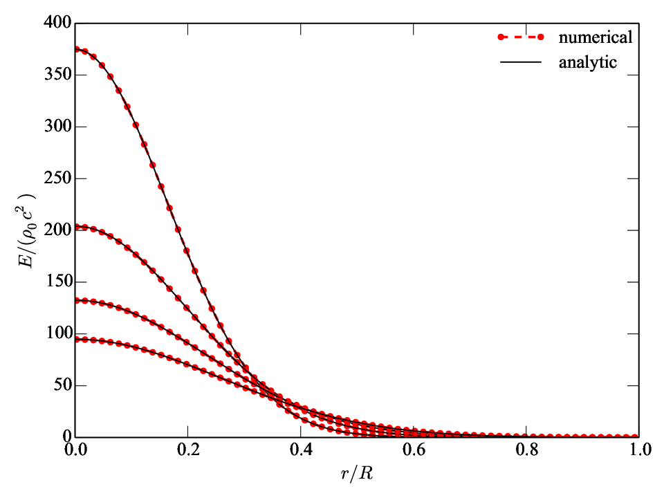
In the opposite optically thick limit, Pons et al. 2000 proposed an analytically tractable problem describing the propagation of a single point source in a strongly diffusive medium. The medium is endowed with zero absorptivity but very high scattering opacity in each frequency bin . For a sufficiently opaque, spherically symmetric medium, the lab-frame energy and flux evolve as a function of radius () and time () according to
| (55) |
| (56) |
The tests presented here fix the grid length to cm, the gas density to g/cm3, and the gas temperature to eV. Specification of the Peclet number , where is a characteristic scale, defines the scattering opacity. We tie the length scale to a small fraction of the grid length and set , safely within the strong scattering limit. All calculations are initialized at and, for the convergence studies, run out to , enough time for the solutions to decay to roughly half of their initial peak energies. Similar to the streaming test, these problems are run with three logarithmically spaced spectral bins ranging from to eV and initialized with spectral energy densities and fluxes such that the frequency-integrated lab frame energy density and flux equate to equations (55) and (56). Results for on a grid with zones are plotted in Figure 2. We find average (maximum) errors of of () and () on grids of and 200 zones, respectively, consistent with a second order convergence rate.
IV.3 Picket Fence
Analytic benchmark solutions for non-equilibrium radiative transfer are scarce, and this is especially true for multi-frequency general relativistic transfer. Hence we occasionally resort, as we do in this section, to the Newtonian literature and limit. As we have emphasized, the radiative transfer algorithms in Cosmos++ are adapted to work in both Newtonian and general relativistic regimes, and because of the covariant nature of the formalism, much of the coding is shared. In fact the only major difference between the two is the primitive inversion scheme, which is not needed for the Newtonian limit. As a result Newtonian problems will exercise much of the general relativistic coding.
One particularly interesting Newtonian problem is the picket-fence proposed by Su & Olson 1999. This test provides a semi-analytic solution for non-grey, two-temperature, non-equilibrium radiative transfer and diffusion, with the caveats that the opacity must be independent of temperature and the material specific heat must be proportional to the cube of the temperature, i.e., . This problem is initialized with a cold, purely absorbing medium, then heated by an extended isotropic radiation source that is a function of space, time and frequency . The source is actually constant over space and time, but active only for a finite duration and over a finite region of space. Hydrodynamic motion (other than thermal coupling) is ignored.
The cold medium is initialized with unit density, unit temperature, and specific heat constant , where is the radiation constant and . The multi-frequency aspect of this test is scripted in the opacity, which is assumed to take one of two values, where , across alternating frequency bins. We use 20 bins to cover (logarithmically) the frequency range to 10 eV, and set the alternating opacities to 2 and 20. The radiating source emits at the rate erg/s/cm3, where K and is the mean opacity, corresponding to Case from Su & Olson 1999. The numerical box size is set to three mean free paths and the radiating source is contained within half a mean free path of the left-most edge of the grid. Figure 3 plots the results at , where is the time measured in units of . The upper panel presents the gas temperature, while the lower panel shows the radiation energies corresponding to the quantities and in the notation of Su & Olson 1999, which represent the total integrated energies across each of the two opacity intervals, i.e., . We also include the benchmark transport solutions as tabulated in Su & Olson 1999. The agreement with the numerical solutions is better than 10% throughout the temperature and energy profiles, a fairly good agreement considering that the closure makes different assumptions than the transport model.

IV.4 Homogeneous Radiating Sphere
We next consider two variants of the homogeneous radiating sphere test (Müller et al. 2010). The basic configuration consists of a static, spherically symmetric, homogeneous, and isothermal stellar sphere of radius , which radiates into a surrounding vacuum region. We assume the dominant interaction process inside the sphere is isotropic absorption and thermal emission with constant absorption opacity and emissivity . Under such conditions, this problem has the following analytic solution (Smit et al. 1997)
| (57) |
where
| (58) |
| (59) |
and is the directional cosine, such that this solution is an integral over all directions. The radiation energy and flux are derived via a numerical integration of the first two moments (angular integrals) of (57).
We set the sphere radius to km and initialize the interior with a constant density g cm-3, a constant temperature with the parametrization , and opacity where is the cell size, is the grid domain length, is the number of grid cells, and is the Peclet number. The exterior background density is fixed at . We consider two parameter sets representing different optical regimes: an optically thinner case (Smit et al. 1997) with , , , and ; and a highly thick case (Abdikamalov et al. 2012) with , , , and . The steady-state solutions for the radiation energies and radial flux-to-energy ratios () are shown in Figure 4 together with the corresponding analytic solutions. The top panels plot the radiation energies, while the bottom panels are the radial flux ratios. The left (right) panels are the optically thinner (thicker) solutions. The qualitative behavior and results compare well to the solutions. We point out, as have previous authors (Smit et al. 1997; O’Connor 2015), that these tests are particularly sensitive to the closure relation which helps explain the deviations observed near the stellar surface. That our numerical methods can handle the discontinuities near the surface and match the asymptotic behavior extremely well is encouraging.


IV.5 Doppler Frequency Shift
The frequency coupling terms from Section III.2 are tested using the same series of calculations as performed by Müller et al. 2010; O’Connor 2015; Kuroda et al. 2016. These tests involve the propagation of radiation from a homogeneous radiating sphere, similar to Section IV.4 except that in addition to isotropic absorption and emission, a sharp velocity profile is added outside the sphere to mimic an accretion flow capable of Doppler redshifting the outgoing radiation.
For all of these tests we set the stellar radius to km, and impose a uniform interior density of g cm-3 and temperature of 5 MeV. The outer radius of the computational box is fixed at km, and in order to resolve both the radiating sphere and Doppler velocity features we use 1080 cells along the radial direction resulting in a grid resolution of km. We choose to run these tests with neutrinos, rather than photons, and with both 15 and 25 frequency bins spanning the range 1-50 MeV. The stellar opacity is made sufficiently thick by setting the Pecklet number to unity over the scale of a single zone. For the velocity profile we use
| (60) |
In this section we consider tests of just the Doppler redshift arising from radiation streaming through the infalling velocity profile of equation (60) without a gravitational potential. However, the same set of analytic solutions are equally applicable to cases with a redshifting potential as we will see in the next section. Variations in the luminosity arise in the free-streaming limit when there are nonzero velocities or potentials, and satisfy the following analytic solution
| (61) |
where is the Lorentz factor, is the lapse function, and the quantity is the luminosity measured by an Eulerian observer and should be constant far from the star. This implies that the mean neutrino energy as measured in the co-moving frame can be calculated as a function of radius
| (62) |
for both Doppler and gravitational redshifts provided the fluid velocity is zero at the star surface and MeV is the mean neutrino energy at the stellar surface. Because of the high stellar opacity we can assume any escaping radiation originates from the stellar surface .
Figure 5 shows the luminosity profile and the mean co-moving frame energy as functions of radius calculated with 25 frequency bins after the radiation achieves steady-state. The corresponding analytic solutions, also plotted in Figure 5, match the numerical results almost exactly everywhere except near the stellar surface where the maximum error in the average photon energy (in the right plot) plateaus at about 3%. However, we point out that the width of the frequency bins near the emission frequency () is MeV, or about . Hence the observed error is within the uncertainty of interpolation between frequency bins, and convergences to zero with increasing frequency resolution, a fact that we have confirmed by running this identical test with a smaller number of frequency bins (15). We note that we importantly observe between first and second order convergence in matching the mean energies at the peak and in the region between the stellar surface and the velocity discontinuity. In particular the maximum errors with 15 (25) frequency bins in the near-surface plateau and Doppler peak regions are 5.3% (3.0%) and 1.6% (0.73%), respectively, corresponding to a convergence rate in frequency of about 1.5.


IV.6 Gravitational Redshift
The problem from the previous section can readily be amended to test gravitational redshifting, too, which we do now. Aside from introducing a self-gravitating potential, all of the problem parameters and the configuration are identical to those specified previously. The potential () is calculated by solving the Newtonian Poisson equation for the uniform density sphere, then assigning the spacetime metric in the spherical, Kerr-Schild gauge as
| (63) |
Figure 6 displays the mean neutrino energy as a function of radius for two cases: pure gravitational redshift (left) and a combination of gravitational plus Doppler redshift with the same velocity profile as specified in Section IV.5 (right). Following the example in that section, we have run each scenario with 15 and 25 frequency bins to verify convergence. The solutions presented in Figure 6 are from the 25-bin tests. The Doppler peaks agree with the analytic solution to better than 1% for both resolutions. As found for the pure Doppler test, agreement is worst right in front of the velocity discontinuity. This region is sensitive to both the spatial and frequency resolutions. Our results with 15 (25) bins nevertheless agree with the analytic solution with maximum errors of about 3.1% (1.5%), converging between first and second order in frequency.


IV.7 Radiation Shock Tube
Most of the tests we consider in this work do not involve both strong kinetic and thermal coupling between the radiation and matter. To address this, we include the following four radiation shock tube tests first introduced by Farris et al. 2008 (Zanotti et al. 2011; Fragile et al. 2012; McKinney et al. 2014, see also): a nonrelativistic strong shock (case 1), a relativistic strong shock (case 2), a relativistic wave (case 3), and a radiation pressure dominated relativistic wave (case 4). The initial parameters are the same as those in Farris et al. 2008 and are reproduced in Table 1. These tests are run until on a grid with 800 zones over . All calculations are run with spectrally uniform energy distributions, , and eighteen frequency groups with bin edges at and , where and come from the initial states of each case. The results are plotted in Figure 7, where we show (in top to bottom order) the gas density, gas pressure, gas velocity, conserved radiation energy, and radiation rest-frame velocity for each case. We point out that we solve these problems using the closure, whereas in most earlier work presenting these tests (Farris et al. 2008; Fragile et al. 2012; Sa̧dowski et al. 2013; Fragile et al. 2014, e.g.), they were solved using the Eddington closure. Not surprisingly, the two closures yield slightly different results, which explains why our new results look different from our previously published ones (we also ran most of the cases to different stop times than before). Only one work that we are aware of, McKinney et al. 2014, has previously published these tests using the closure, so our results should be compared with those, and, in fact, we find the agreement to be excellent.
| Case | ||||||||||
|---|---|---|---|---|---|---|---|---|---|---|
| 1 | 5/3 | 0.4 | 1 | 2.4 | ||||||
| 2 | 5/3 | 0.2 | 1 | 0.25 | 3.11 | |||||
| 3 | 2 | 0.3 | 1 | 10 | 2 | 8 | ||||
| 4 | 5/3 | 0.08 | 1 | 0.69 | 0.18 | 3.65 |


IV.8 Shadow Casting
An important advantage of closure over the diffusion (or isotropic Eddington) approximation is its ability to preserve shadows in the wake of opaque objects. In a previous paper (Fragile et al. 2014) we demonstrated this ability with our grey (single group) version of . In that paper we considered radiation flow across an opaque spheroidal cloud embedded in a low density transparent medium with a light source placed at one end of the computational domain. Here we generalize that test problem by replacing the spheriodal cloud with a density-stratified slab. As we will demonstrate, density stratification serves to exercise the multi-frequency capabilities of our new transport algorithm.
Four density layers are utilized in this test, along with three frequency groups. The background (transparent medium) density is fixed at g cm-3, while the opaque object is layered (from the bottom up) with densities of , , and g cm-3. The opaque slab is 1 cm long by 1 cm tall and rests 0.5 cm along the bottom of a grid cm long by cm tall, resolved with zones. Each density layer is cm thick. The gas and radiation begin in cold equilibrium with with a gas adiabatic index of . The photon streams are initialized at the left boundary with a uniform (frequency-integrated) source temperature = 1740 K, so that and . Spectral energies and fluxes are initialized as and , where is the number of frequency bins.
The opacity of the gas is designed to produce the desired behavior of the bin-center energies through the different density layers. In particular, the frequency bin edges ( and 2 eV), the number of frequency groups (3, with logarithmic spacing), the opacity parameters, and the density layers are tailored so that each stacked layer of the slab is optically thin to a different frequency bin so that we can test shadow casting for each individual frequency group. This is accomplished with the following absorption opacity power law (we do not consider scattering here):
| (64) |
where the coefficient is chosen to normalize the mean free path of the highest frequency photons through the densest (inner) layer to cm, thus guaranteeing that the slab is sufficiently opaque in its bottom layer to block all streaming photons. Furthermore, the combination of densities and opacity power-law parameters define essentially the same optical thickness to the middle frequency photons in the middle layer, and to the lowest frequency photons in the topmost layer.
From this configuration we expect to observe the following: all photons will be blocked by the bottom (highest density) layer; photons in the two lowest frequency bins will be blocked in the middle layer; only the lowest frequency photons will be blocked in the upper layer; and all photons will stream through the low density gap above the opaque slab. Hence we should see a clear separation of photon streams and shadows if we plot each frequency bin separately. The results, after 1.5 light-crossing times, as shown in Figure 8, confirm these expectations. The three images plot for the three photon bin center frequencies, at roughly 0.01, 0.1 and 1 eV. As expected, the density layers produce sharp, clear shadows in both space and spectral energy. Notice that, as the radiation propagates, the edges of the shadows tend to flare out, a trait that is sensitive to the reconstruction method and limiter steepness (Davis et al. 2012; McKinney et al. 2014), yet the transition from light to dark is nevertheless quite pronounced at all frequencies. To demonstrate the clean separation of the three spectral components after passing through the stratified slab, we plot in Figure 9 the average photon energy as a function of the vertical height, , crossing the horizontal position cm. Also plotted is an “analytic” solution that is calculated by only summing the energy within the bin ranges that are theoretically transparent for a given height. The agreement is quite good.


IV.9 Two-Beam Shadow Test
The shadow test from the previous section demonstrates one advantage of the closure scheme over simpler flux-limited diffusion, the fact that it accurately casts shadows from a single beam incident upon an opaque object. However, a well-known shortcoming of flux-integrated (grey) is that intersecting beams of light do not correctly cross one another. Instead, they merge, flowing in the direction of the average, resultant flux. A traditional illustration of this is the two-beam, shadow test (Sa̧dowski et al. 2013; Fragile et al. 2014; McKinney et al. 2014). In this test, two beams of radiation enter the computational domain, one from the upper and one from the lower boundaries. Each beam is angled toward a circular cloud along the centerline of the grid. Rather than the two beams casting two independent shadows as would be expected, they cast three partial shadows, one each in the directions of the original beams, and one in the “average” beam direction. This third shadow is the unphysical result of the partial merging of the two beams.
While our current multi-frequency radiation transport does not provide a true solution to the issue of merging beams, it does admit an interesting workaround. Since photons (or beams) in different frequency bins are advected independently, and since there is no process in this test to trigger frequency exchanges, two beams of different frequencies can propagate independently, cross as expected, and cast individual shadows as they should. To illustrate this, we repeat the two-beam shadow test as presented in Sa̧dowski et al. 2013; Fragile et al. 2014, but with the new twist that each beam occupies a different frequency bin (the bin boundaries are not relevant). The test is run on a grid, obviously with no reflection applied at . Figure 10 confirms our expectation that the two beams now leave only two shadows, one in each of the beam directions. Interestingly, since Figure 10 shows the frequency-integrated radiation energy and velocity, the beams appear to merge in the red triangular regions, but are actually still traveling in their independent directions.

IV.10 Beam of Light Near a Black Hole
An important test for a general relativistic radiation transport scheme is to verify that the radiation propagates along geodesics as expected in strong gravitational fields. To verify this, we reproduce a series of light beam tests introduced by Sa̧dowski et al. 2013. For these tests we initialize a photon beam in the curved spacetime geometry near a Schwarzschild black hole, and neglect any coupling interactions between the gas and radiation () so that we can compare the path of the radiation beam against accurate geodesic paths. In this section, all distances are measured in units of . All calculations are run with 5 frequency groups covering 10 to eV on a two-dimensional grid, with resolution and grid coverage over and . We consider two cases: () = (2.5, 3.5, 3.0) and (5.5, 11.5, 6), where defines the beam center and width. Note that the beam in the first case is centered at the photon orbit radius, , meaning that photons in the center of the beam should be able to orbit the black hole indefinitely. The radiation temperature within the initial beam is K, where is the temperature of the background radiation. The radiation beam has an initial Lorentz factor of in the grid frame. The beam initial conditions are held constant at the boundary.
Figure 11 shows the track of each radiation beam summed over all frequency bins, i.e., , along with geodesic paths corresponding to the initial inner and outer boundaries of each beam. The left image corresponds to the photon orbit case with , while the right corresponds to . We see that each beam stays confined within the prescribed geodesic tracks and experiences the expected curvature. Furthermore, each frequency group experiences the same curvature, so that the beam intensity is independent of the number of groups.


V Conclusion
In this work, we have extended the capabilities of our Cosmos++ computational astrophysics code to include multi-frequency radiation. This is done by selecting a finite number of frequency groups and independently evolving the radiation energy densities and momenta associated with each. We stick with the same explicit-implicit split of advection and radiation source terms and the two-moment closure scheme as our previous work (Fragile et al. 2014). Thus, we retain the ability to stably evolve a large range of parameter space from optically thin to optically thick flows with reasonable time steps and accuracy, while now relaxing the grey (frequency-integrated) approximation. In this work, we have focused on presenting and testing the general relativistic version, though we note that we have also implemented a Newtonian version as well. We also have a multi-group, flux-limited-diffusion option, which we plan to report on elsewhere.
This multi-frequency capability expands the range of physical processes that can be properly captured in a simulation. For example, we demonstrated how the new code could successfully treat frequency-dependent opacities and Doppler and gravitational frequency shifts, and to some extent overcome the multi-beam shadowing limitations of the closure scheme.
While multi-frequency methods are already in use in studies of core-collapse supernovae (Just et al. 2015; Kuroda et al. 2016, e.g.,), they have many potential uses beyond that class of problem. Possible applications include Type Ia supernovae, neutron star mergers, tidal disruption events, and super-Eddington accretion onto compact objects. Another potential application is in the study of black hole X-ray binary accretion disks, especially in the so-called intermediate spectral states, where hard and soft X-ray photons each play important roles, not only in the observed spectra, but in physically interacting with the accretion flow, affecting its structure and thermodynamic state. It is important in such an application for hard and soft X-ray photons to be able to propagate independently, experience the expected gravitational and Doppler frequency shifts, follow proper geodesic paths, and interact with the gas in a frequency-dependent manner – all of the capabilities we have demonstrated in this paper.
Appendix A 1st Order Taylor Expansion Terms
The Jacobian matrix, , from Section III.3 can either be calculated analytically or numerically. Although more tedious to code, we have found that the analytic method is consistently faster on all our tests, making it perhaps worth the extra effort. To aid those who might wish to code the analytic solution, we record all the pertinent partial derivatives for equation (53) here, ordered by conserved field. Notice we have dropped the frequency subscript notation in most of these expressions, but emphasize that radiation related derivatives apply to all groups.
Mass density:
Fluid energy:
Fluid momentum:
Radiation energy:
Radiation momentum:
Also appearing in the Jacobian are the following gradients of the radiation 4-force density:
Finally, the following partial derivatives are needed to evaluate the above expressions:
References
- Aartsen et al. (2019) Aartsen, M. G., Ackermann, M., Adams, J., et al. 2019, arXiv e-prints, arXiv:1911.02561
- Abbot et al. (2017) Abbot, B. P., et al. 2017, ApJ, 848, L12
- Abbot et al. (2018) —. 2018, Living Reviews in Relativity, 21, 3
- Abdikamalov et al. (2012) Abdikamalov, E., Burrows, A., Ott, C. D., et al. 2012, ApJ, 755, 111
- Abramowicz & Fragile (2013) Abramowicz, M. A., & Fragile, P. C. 2013, Living Reviews in Relativity, 16, 1
- Anninos et al. (2017) Anninos, P., Bryant, C., Fragile, P. C., et al. 2017, ApJS, 231, 17
- Anninos et al. (2005) Anninos, P., Fragile, P. C., & Salmonson, J. D. 2005, ApJ, 635, 723
- Burke-Spolaor (2018) Burke-Spolaor, S. 2018, Nature Astronomy, 2, 845
- Burns et al. (2019) Burns, E., et al. 2019, ApJ, 871, 90
- Burrows (2013) Burrows, A. 2013, Reviews of Modern Physics, 85, 245
- Chambers et al. (2016) Chambers, K. C., Magnier, E. A., Metcalfe, N., et al. 2016, arXiv e-prints, arXiv:1612.05560
- Charles & Shaw (2013) Charles, P., & Shaw, A. 2013, Astronomy and Geophysics, 54, 6.15
- Cherenkov Telescope Array Consortium et al. (2019) Cherenkov Telescope Array Consortium, Acharya, B. S., Agudo, I., et al. 2019, Science with the Cherenkov Telescope Array (World Scientific Publishing Co. Pte. Ltd.)
- Dai et al. (2018) Dai, L., McKinney, J. C., Roth, N., Ramirez-Ruiz, E., & Miller, M. C. 2018, ApJ, 859, L20
- Davis & Gammie (2020) Davis, S. W., & Gammie, C. F. 2020, ApJ, 888, 94
- Davis et al. (2012) Davis, S. W., Stone, J. M., & Jiang, Y.-F. 2012, ApJS, 199, 9
- Dubroca & Feugeas (1999) Dubroca, B., & Feugeas, J. 1999, Academie des Sciences Paris Comptes Rendus Serie Sciences Mathematiques, 329, 915
- Fang et al. (2019) Fang, K., Metzger, B. D., Murase, K., Bartos, I., & Kotera, K. 2019, ApJ, 878, 34
- Farris et al. (2008) Farris, B. D., Li, T. K., Liu, Y. T., & Shapiro, S. L. 2008, Phys. Rev. D, 78, 024023
- Foglizzo et al. (2015) Foglizzo, T., Kazeroni, R., Guilet, J., et al. 2015, PASA, 32, e009
- Foucart et al. (2016a) Foucart, F., O’Connor, E., Roberts, L., et al. 2016a, Phys. Rev. D, 94, 123016
- Foucart et al. (2015) —. 2015, Phys. Rev. D, 91, 124021
- Foucart et al. (2016b) Foucart, F., Haas, R., Duez, M. D., et al. 2016b, Phys. Rev. D, 93, 044019
- Fragile et al. (2020) Fragile, P. C., Ballantyne, D. R., & Blankenship, A. 2020, Nature Astronomy, 6
- Fragile et al. (2018a) Fragile, P. C., Ballantyne, D. R., Maccarone, T. J., & Witry, J. W. L. 2018a, ApJ, 867, L28
- Fragile et al. (2018b) Fragile, P. C., Etheridge, S. M., Anninos, P., Mishra, B., & Kluźniak, W. 2018b, ApJ, 857, 1
- Fragile et al. (2012) Fragile, P. C., Gillespie, A., Monahan, T., Rodriguez, M., & Anninos, P. 2012, ApJS, 201, 9
- Fragile et al. (2014) Fragile, P. C., Olejar, A., & Anninos, P. 2014, ApJ, 796, 22
- Gammie et al. (2003) Gammie, C. F., McKinney, J. C., & Tóth, G. 2003, ApJ, 589, 444
- González et al. (2007) González, M., Audit, E., & Huynh, P. 2007, A&A, 464, 429
- González et al. (2015) González, M., Vaytet, N., Commerçon, B., & Masson, J. 2015, A&A, 578, A12
- Graham et al. (2019) Graham, M. J., Kulkarni, S. R., Bellm, E. C., et al. 2019, PASP, 131, 078001
- IceCube Collaboration et al. (2018) IceCube Collaboration, Aartsen, M. G., Ackermann, M., et al. 2018, Science, 361, eaat1378
- Ivezić et al. (2019) Ivezić, Ž., Kahn, S. M., Tyson, J. A., et al. 2019, ApJ, 873, 111
- Janka (2012) Janka, H.-T. 2012, Annual Review of Nuclear and Particle Science, 62, 407
- Jiang et al. (2012) Jiang, Y.-F., Stone, J. M., & Davis, S. W. 2012, ApJS, 199, 14
- Just et al. (2015) Just, O., Obergaulinger, M., & Janka, H. T. 2015, MNRAS, 453, 3386
- Keivani et al. (2018) Keivani, A., Murase, K., Petropoulou, M., et al. 2018, ApJ, 864, 84
- Kuroda et al. (2016) Kuroda, T., Takiwaki, T., & Kotake, K. 2016, ApJS, 222, 20
- Lentz et al. (2012) Lentz, E. J., Mezzacappa, A., Bronson Messer, O. E., et al. 2012, ApJ, 747, 73
- Levermore (1984) Levermore, C. D. 1984, JQSRT, 31, 149
- Levermore & Pomraning (1981) Levermore, C. D., & Pomraning, G. C. 1981, ApJ, 248, 321
- McKinney et al. (2014) McKinney, J. C., Tchekhovskoy, A., Sadowski, A., & Narayan, R. 2014, MNRAS, 441, 3177
- Metzger (2017) Metzger, B. D. 2017, arXiv e-prints, arXiv:1710.05931
- Mishra et al. (2016) Mishra, B., Fragile, P. C., Johnson, L. C., & Kluźniak, W. 2016, MNRAS, 463, 3437
- Müller et al. (2010) Müller, B., Janka, H.-T., & Dimmelmeier, H. 2010, ApJS, 189, 104
- O’Connor (2015) O’Connor, E. 2015, ApJS, 219, 24
- Pareschi & Russo (2001) Pareschi, L., & Russo, G. 2001, in Recent Trends in Numerical Analysis, Vol. 3 (Hauppauge, New York: Nova Scientific Publishers), 269–288
- Pomraning (1981) Pomraning, G. C. 1981, J. Quant. Spec. Radiat. Transf., 26, 385
- Pons et al. (2000) Pons, J. A., Ibanez, J. M., & Miralles, J. A. 2000, MNRAS, 317, 550
- Ryan & Dolence (2020) Ryan, B. R., & Dolence, J. C. 2020, ApJ, 891, 118
- Sa̧dowski et al. (2013) Sa̧dowski, A., Narayan, R., Tchekhovskoy, A., & Zhu, Y. 2013, MNRAS, 429, 3533
- Sekiguchi et al. (2016) Sekiguchi, Y., Kiuchi, K., Kyutoku, K., Shibata, M., & Taniguchi, K. 2016, Phys. Rev. D, 93, 124046
- Senno et al. (2017) Senno, N., Murase, K., & Mészáros, P. 2017, ApJ, 838, 3
- Shibata et al. (2011) Shibata, M., Kiuchi, K., Sekiguchi, Y., & Suwa, Y. 2011, Progress of Theoretical Physics, 125, 1255
- Skinner et al. (2019) Skinner, M. A., Dolence, J. C., Burrows, A., Radice, D., & Vartanyan, D. 2019, ApJS, 241, 7
- Smit et al. (1997) Smit, J. M., Cernohorsky, J., & Dullemond, C. P. 1997, A&A, 325, 203
- Su & Olson (1999) Su, B., & Olson, G. L. 1999, Journal of Quantitative Spectroscopy and Radiative Transfer, 62, 279
- Takahashi et al. (2016) Takahashi, H. R., Ohsuga, K., Kawashima, T., & Sekiguchi, Y. 2016, ApJ, 826, 23
- Thorne (1981) Thorne, K. S. 1981, MNRAS, 194, 439
- Tominaga et al. (2015) Tominaga, N., Shibata, S., & Blinnikov, S. I. 2015, ApJS, 219, 38
- Wang et al. (2020) Wang, M.-H., Ai, S.-K., Li, Z.-X., et al. 2020, ApJ, 891, L39
- Weih et al. (2020) Weih, L. R., Olivares, H., & Rezzolla, L. 2020, MNRAS
- Zanotti et al. (2011) Zanotti, O., Roedig, C., Rezzolla, L., & Del Zanna, L. 2011, MNRAS, 417, 2899
- Zhang et al. (2013) Zhang, W., Howell, L., Almgren, A., et al. 2013, ApJS, 204, 7