∎

Online Robust and Adaptive Learning from Data Streams

Shintaro Fukushima Affiliation: Graduate School of Information Science and Technology, The University of Tokyo
7-3-1 Hongo, Bunkyo-ku, Tokyo, Japan
TOYOTA MOTOR CORPORATION
1-6-1 Otemachi, Chiyoda-ku, Tokyo, Japan E-mail: sfukushim@gmail.com s_fukushima@mail.toyota.co.jp Atsushi Nitanda Affiliation: Faculty of Computer Science and Systems Engineering, Kyushu Institute of Technology
680-4 Kawazu, Iizuka-shi, Fukuoka, Japan E-mail: nitanda@ai.kyutech.ac.jp Kenji Yamanishi Affiliation: Graduate School of Information Science and Technology, The University of Tokyo
7-3-1 Hongo, Bunkyo-ku, Tokyo, Japan E-mail: yamanishi@gcc.e.u-tokyo.ac.jp

Received: date / Accepted: date

Abstract

In online learning from non-stationary data streams, it is necessary to learn robustly to outliers and to adapt quickly to changes in the underlying data generating mechanism. In this paper, we refer to the former attribute of online learning algorithms as robustness and to the latter as adaptivity. There is an obvious tradeoff between the two attributes. It is a fundamental issue to quantify and evaluate the tradeoff because it provides important information on the data generating mechanism. However, no previous work has considered the tradeoff quantitatively. We propose a novel algorithm called the stochastic approximation-based robustness-adaptivity algorithm (SRA) to evaluate the tradeoff. The key idea of SRA is to update parameters of distribution or sufficient statistics with the biased stochastic approximation scheme, while dropping data points with large values of the stochastic update. We address the relation between the two parameters: one is the step size of the stochastic approximation, and the other is the threshold parameter of the norm of the stochastic update. The former controls the adaptivity and the latter does the robustness. We give a theoretical analysis for the non-asymptotic convergence of SRA in the presence of outliers, which depends on both the step size and threshold parameter. Because SRA is formulated on the majorization-minimization principle, it is a general algorithm that includes many algorithms, such as the online EM algorithm and stochastic gradient descent. Empirical experiments for both synthetic and real datasets demonstrated that SRA was superior to previous methods. As SRA is based on assumptions that an abrupt change occurs in parameters or sufficient statistics of true distribution and that noisy distribution obeys the uniform distribution, it would be expected for SRA to be theoretically guaranteed in more general settings, such as incremental (gradual) changes and other noisy distributions.

Keywords:

Online learning Outlier Change point Data stream Stochastic approximation Expectation-Maximization algorithm

1 Introduction

1.1 Purpose of this paper

This study is concerned with online learning from data streams. We consider a situation where each datum arrives in an online fashion. In such a situation, we aim to (i) learn robustly to outliers or anomalies in the observed data. (ii) adapt to the changes in the underlying data-generating mechanism. In (i), if a data point is an outlier, we would like to learn with as little influence by the outlier as possible. In this paper, we refer to such an attribute of online learning algorithms as robustness. In contrast, with regard to (ii), it is desirable to adapt to the changes in the data-generating mechanism. We refer to such an attribute of online learning algorithms as adaptivity. Figure 1 illustrates the concepts of the robustness and adaptivity.

Figure 1: Illustration of the concepts of the robustness and adaptivity of online learning algorithms.

A tradeoff exists between the robustness and adaptivity: the robustness generally decreases if we try to adapt to the changes. Conversely, the adaptivity decreases if we try to learn robustly. Although many online learning algorithms have been introduced and some studies have addressed this issue (Tsay 1988; Gama et al. 2014; Chu et al. 2004; Huang et al. 2016; Odakura 2018; Cejnek and Bukovsky 2018; Fearnhead and Rigaill 2019; Guo 2019), to the best of our knowledge, no algorithm has quantitatively considered the tradeoff between the robustness and adaptivity.

This study proposes an online learning algorithm that considers the tradeoff between the robustness and adaptivity. We introduce a novel algorithm, called the stochastic approximation-based robustness–adaptivity (SRA) algorithm, to provide a theoretical analysis for non-asymptotic convergence of SRA in the presence of outliers and to demonstrate its effectiveness for both synthetic and real datasets. The key idea of SRA is to update parameters of distribution or sufficient statistics with the stochastic approximation (SA) (Robbins and Monro 1951) while dropping points with large values of stochastic updates (drift terms).

1.2 Related work

This study is concerned with the robustness and adaptivity of online learning algorithms. Moreover, we briefly review studies related to the SA (Robbins and Monro 1951) and the online expectation–maximization (EM) algorithm (Cappé and Moulines 2009; Karimi et al. 2019a) because SRA uses both of them.

1.2.1 Robustness and adaptivity of online learning algorithms

The robustness and adaptivity of online learning algorithms have often been discussed in the context of the concept drift (Gama et al. 2014; Chu et al. 2004; Huang et al. 2016; Cejnek and Bukovsky 2018). Yamanishi et al. proposed an online learning algorithm, called the sequentially discounting EM algorithm (SDEM) (Yamanishi et al. 2004). Although SDEM can handle complicated distributions, it is prone to noise and can easily overfit the data. Odakura proposed an online nonstationary robust learning algorithm (Odakura 2018). This algorithm independently introduces two parameters to control the robustness and adaptivity, respectively. Fearnhead and Rigaill proposed an algorithm for change detection that is robust in the presence of outliers (Fearnhead and Rigaill 2019). The key idea of the algorithm is to adapt existing penalized cost approaches to detect changes such that the loss function is less sensitive to outliers. Guo proposed an algorithm based on an online sequential extreme learning machine for robust and adaptive learning (Guo 2019).

1.2.2 Online (stochastic) EM algorithms

The EM algorithm (Dempster et al. 1977) is a popular class of inference that minimizes loss function. The original EM algorithm does not scale to a large dataset because it requires the entire data at each iteration. To overcome this problem, several studies proposed online versions of the EM algorithm.

Neal and Hinton proposed an EM algorithm in an incremental scheme referred to as the incremental EM (iEM) (Neal and Hinton 1999). Cappé and Moulines proposed the stochastic (online) EM (sEM) algorithm (Cappé and Moulines 2009), which updates the sufficient statistics in an SA scheme (Robbins and Monro 1951). Chen et al. proposed the variance reduced sEM (sEM-VR) algorithm (Chen et al. 2018). Meanwhile, Karimi et al. showed non-asymptotic convergence bounds for the global convergence of iEM, sEM-VR, and the fast incremental EM (Karimi et al. 2019b).

By contrast, only a few studies have considered the online EM algorithm in a situation where a fresh sample is drawn at each iteration. Cappé and Moulines proved the asymptotic convergence of the online EM algorithm (Cappé and Moulines 2009). Balakrishnan et al. analyzed the non-asymptotic convergence for a variant of the online EM algorithm (Balakrishnan et al. 2017), where the initial radius around the optimal parameter must be known in advance. Karimi et al. considered the SA scheme (Robbins and Monro 1951), the stochastic update (drift term) of which depends on a state-dependent Markov chain. Moreover, the mean field is not necessarily of a gradient type, thereby covering an approximate second-order method and allowing an asymptotic bias for one-step updates (Karimi et al. 2019a). They illustrated these settings using the online EM algorithm and the policy-gradient method for the average reward maximization in reinforcement learning.

1.3 Significance of this paper

In the context of Section 1.1 and 1.2, the contributions of this paper are summarized below.

1.3.1 Novel online learning algorithm for tradeoff between robustness and adaptivity

We propose a novel online learning algorithm, called SRA, to consider the tradeoff between the robustness and adaptivity. Previous studies (Chu et al. 2004; Huang et al. 2016; Cejnek and Bukovsky 2018; Yamanishi et al. 2004; Odakura 2018; Fearnhead and Rigaill 2019; Guo 2019) considered only one of them, and even when both were considered, the relation between them was not clarified. This study considers both the robustness and adaptivity, and gives a theoretical analysis for the non-asymptotic convergence of SRA. To do so, we adopt the SA scheme (Robbins and Monro 1951) in a setting where outliers and change points may exist. As SRA is formulated on the majorization–minimization principle (Lange 2016; Mairal 2015), it is a general algorithm that includes many schemes, such as the online EM algorithm (Cappé and Moulines 2009; Balakrishnan et al. 2017; Karimi et al. 2019a) and stochastic gradient descent (SGD). Our approach is considered to be an extension of the work of (Karimi et al. 2019a), but they presented convergence analysis of the biased SA in the absence of outliers and change points. By contrast, we consider convergence analysis in a setting where outliers and change points may exist. Our study is novel in that we show non-asymptotic convergence analysis in this broader setting and apply it to quantify and evaluate the tradeoff between the robustness and adaptivity of online learning algorithms.

We present a detailed comparison between one of the promising previous studies and this study, to clarify the advantages of this study over previous ones. Fearnhead and Rigaill proposed a promising algorithm called F-RPOP for change detection in the presence of outliers (Fearnhead and Rigaill 2019). The key idea of F-RPOP is to find the optimal segmentation (change points) of a data stream with dynamic programming under penalized cost criteria. More specifically, the authors defined the cost of a segment as the sum of losses at the time points in the segment using a loss function, and then found the optimal segmentation (change points) by minimizing the cost with dynamic programming. The loss function has a segment-specific location parameter $\theta$ . Some loss functions also have parameter $K$ , that is, the tolerance threshold of distance between a data point and $\theta$ . The functions include the Huber loss and the biweight loss. Therefore, $K$ controls the robustness. The authors also introduced a parameter $\beta$ in dynamic programming, which affects the number of change points. Therefore, $\beta$ controls the adaptivity. However, the relation between $K$ and $\beta$ is not clarified in (Fearnhead and Rigaill 2019) except one on the lengths of segments. Although empirical studies show good results with the robustness and adaptivity, it is necessary to tune the two parameters $K$ and $\beta$ separately without the knowledge of the relation on the robustness and adaptivity between them. By contrast, this study quantitatively evaluates the tradeoff between the robustness and adaptivity. From an empirical point of view, this evaluation leads to the relation between two parameters that control the robustness and adaptivity. When a value of one parameter is given, the value of the other parameter is determined theoretically.

Note that many studies already addressed the tradeoff between exploration and exploitation in bandit algorithms (e.g., (Lattimore and Szepesväri 2018)). However, our problem setting is different from those in these studies. Bandit algorithms search for parameters independently of changes in the environment. In contrast, our SRA does not greatly change parameters when the change in the data-generating mechanism is moderate. It adapts to the changes of the data-generating mechanism. Therefore, although both our study and those concerned with bandit algorithms consider the tradeoff between global and local information, our motivation is different from that in other studies.

1.3.2 Empirical demonstration of the proposed algorithm

We evaluated the effectiveness of SRA on both synthetic and real datasets. We empirically showed characteristics of SRA by inspecting the dependencies on the parameters of SRA; these were consistent with those of the theoretical analysis. We also compared the performance of SRA with those of the previously proposed online learning algorithms (Neal and Hinton 1999; Yamanishi et al. 2004; Cappé and Moulines 2009) and concep drift detection algorithms (Bifet and Gavaldá 2007; Raab et al. 2020; Page 1954) , on important tasks, including change detection and anomaly detection. It was determined that SRA was superior to other algorithms.

2 Preliminaries

In this section, we provide our problem setting and an important theoretical result of previous study: non-asymptotic convergence of SA Karimi et al. 2019a.

2.1 Problem setting

We consider a situation where each datum $y_{t}\in\mathbb{R}^{d}$ arrives in an online fashion at each time $t\in\mathbb{N}$ . If no noise exists, we assume that $y_{t}$ is drawn from

\displaystyle y_{t}\sim f(y_{t};\theta_{t}),

(1)

where $f\in\mathcal{F}$ is an element of a parametric class of distribution $\mathcal{F}=\{f(y;\theta),\,\theta\in\Theta\}$ , $\theta$ is a parameter, and $\Theta\subset\mathbb{R}^{p}$ is a parameter space associated. However, in the real world, data are sometimes contaminated by noise. In this case, we assume that $y_{t}$ is drawn from a mixture of probability density functions:

\displaystyle y_{t}\sim\alpha f(y_{t};\theta_{t})+(1-\alpha)f_{\mathrm{noise}}(y_{t};\xi),

(2)

where $\alpha$ denotes the mixture ratio ( $0<\alpha<1$ ). Equation (2) means that a datum is generated from a true distribution with probability $\alpha$ and from a noisy distribution with probability $1-\alpha$ . $f_{\mathrm{noise}}$ is an element of a parametric class of data distributions $\mathcal{G}=\{f_{\mathrm{noise}}(y;\xi),\,\xi\in\Xi\}$ , where $\xi$ is a parameter and $\Xi\subset\mathbb{R}^{m}$ is a parameter space associated. This study addresses the convergence property of Equation (2).

We assume that a change point $t^{\ast}$ is given, and each datum before and after the change point is drawn from different distributions. This means that $\theta_{t}$ in Equation (2) varies as follows:

\displaystyle\theta_{t}=\left\{\begin{array}[]{ll}\theta^{1}&(t=1,\dots,t^{\ast}-1),\\ \theta^{2}&(t=t^{\ast},\dots),\end{array}\right.

where $\theta^{1}\neq\theta^{2}$ . This implies a change abruptly occurs at $t^{\ast}$ .

2.2 Non-asymptotic analysis of SA

Karimi et al. showed a convergence analysis (Karimi et al. 2019a) of the non-convex objective function under the SA scheme (Robbins and Monro 1951) in Equation (1):

\displaystyle\theta_{t+1}=\theta_{t}-\rho_{t+1}H_{\theta_{t}}(Y_{t+1}),

(5)

where $\theta_{t}\in\Theta\subset\mathbb{R}^{p}$ denotes the $t$ -th iterate of parameters or the sufficient statistics of the distribution, $\rho_{t+1}$ is the step size. $Y_{t+1}$ denotes the random variable at $t+1$ , and $y_{t+1}$ does its realization. $H_{\theta_{t}}(Y_{t+1})$ is the stochastic update at time $t$ . When $\{y_{t}\}_{t=1}^{\infty}$ is an i.i.d. sequence of random vectors, the mean field for the SA is defined as $h(\theta_{t})=\mathbb{E}[H_{\theta_{t}}(Y_{t+1})|\mathcal{F}_{t}]$ , where $\mathcal{F}_{t}$ is the filtration generated by the random variables $(\theta_{0},\{Y_{s}\}_{s=1}^{t})$ , at time $t$ . When $\{y_{t}\}_{t=1}^{\infty}$ is a state-dependent Markov chain, $h(\theta_{t})=\int H_{\theta_{t}}(y)\,\pi_{\theta_{t}}(\mathrm{d}y)$ under the assumption that $\int\|H_{\theta_{t}}(y)\|\,\pi_{\theta_{t}}(\mathrm{d}y)<\infty$ , where $\|\cdot\|$ denotes the norm of the vector in $\mathbb{R}^{p}$ and $\pi=\pi_{\theta}(y)$ is the true distribution. In this study, we consider the former case, that is, $\{y_{t}\}_{t=1}^{\infty}$ is an i.i.d sequence of random vectors. Karimi et al. assumed that $h$ is related to a smooth Lyapunov function $V:\mathbb{R}^{p}\rightarrow\mathbb{R}$ , where $V(\theta)>-\infty$ . This SA scheme in Equation (5) aims to find a minimizer or a stationary point of the non-convex Lyapunov function $V$ .

For example, let us consider the online EM algorithm (Cappé and Moulines 2009; Karimi et al. 2019a) to the curved exponential family:

\displaystyle f(Y,Z;\theta)=h(Y,Z)\exp{\left(\langle S(Y,Z)|\phi(\theta)\rangle-\psi(\theta)\right)}.

(6)

Here, $\psi:\Theta\rightarrow\mathbb{R}$ is twice differentiable and convex. $\phi:\Theta\rightarrow\mathrm{S}\subset\mathbb{R}^{p}$ is concave and differentiable. $\mathrm{S}$ is a convex open subset of $\mathbb{R}^{p}$ , $S$ denotes the sufficient statistics, and $\langle\cdot|\cdot\rangle$ denotes dot product. The Lyapunov function $V(s)$ is defined for the sufficient statistics $s$ as

\displaystyle V(s)\mathrel{\overset{\makebox[0.0pt]{\mbox{\tiny def}}}{=}}\mathrm{KL}(\pi,g(\cdot;\bar{\theta}(s)))+R(\bar{\theta}(s)),

(7)

where $\mathrm{KL}$ is Kullback–Leibler (KL) divergence between $\pi$ and $g_{\theta}$ defined as

\displaystyle\mathrm{KL}(\pi,g)

\displaystyle\mathrel{\overset{\makebox[0.0pt]{\mbox{\tiny def}}}{=}}\mathbb{E}_{\pi}[\log{(\pi(Y)/g(Y;\theta))}],

(8)

and $R:\Theta\rightarrow\mathbb{R}$ is a penalization term assumed to be twice differentiable (Karimi et al. 2019a). $\bar{\theta}$ in Equation (7) is defined as the minimizer of the following loss function:

\displaystyle\ell(s;\theta)=\psi(\theta)+R(\theta)-\langle s|\phi(\theta)\rangle.

(9)

Therefore, $\bar{\theta}(s)$ is represented as

\displaystyle\bar{\theta}(s)\mathrel{\overset{\makebox[0.0pt]{\mbox{\tiny def}}}{=}}\operatornamewithlimits{argmin}_{\theta}\,\ell(s;\theta)=\operatornamewithlimits{argmin}_{\theta}\,\left\{\psi(\theta)+R(\theta)-\langle s|\phi(\theta)\rangle\right\}.

(10)

Karimi et al. considered the following assumptions for $h$ and $V$ .

Assumption 1

(Karimi et al. 2019a)

(a): $\forall\theta\in\Theta$ , $\exists c_{0}\geq 0,\,c_{1}>0$ , s.t. $c_{0}+c_{1}\langle\nabla V(\theta)|h(\theta)\rangle\geq\|h(\theta)\|^{2}$ .
(b): $\forall\theta\in\Theta$ , $\exists d_{0}>0,d_{1}>0$ , s.t. $d_{0}+d_{1}\|h(\theta)\|\geq\|\nabla V(\theta)\|$ .
(c): The Lyapunov function $V$ is L-smooth: $\forall(\theta,\theta^{\prime})\in\Theta^{2},\|\nabla V(\theta)-\nabla V(\theta^{\prime})\|\leq L\|\theta-\theta^{\prime}\|$ .

Here, $\|h(\theta)\|$ denotes the norm of the mean field which takes on small values as the SA scheme in Equation (5) converges. Assumption 1 (a) and (b) assume that the mean field $h(\theta)$ is indirectly related to the Lyapunov function $V(\theta)$ , but it is not necessarily the same as $\nabla V(\theta)$ . The constants $c_{0}$ and $d_{0}$ characterize the bias between the mean field and the gradient of the Lyapunov function. We note that the Lyapunov function $V$ can be a non-convex function under Assumption 1 (c).

For any $n\geq 1$ , we denote $N\in\{0,\dots,n\}$ as a discrete random variable independent of $\{\mathcal{F}_{n}\}_{n=1}^{\infty}$ . When we adopt a randomized stopping rule in SA as in (Ghadimi and Lan 2013), we define $P(N=\ell)\mathrel{\overset{\makebox[0.0pt]{\mbox{\tiny def}}}{=}}\rho_{\ell+1}/\sum_{k=0}^{n}\rho_{k+1}$ , where $N$ is the terminating iteration for Equation (5). We consider the following expectation:

\displaystyle\mathbb{E}[\|h(\theta_{N})\|^{2}]=\sum_{k=1}^{n}P(N=k)\|h(\theta_{k})\|^{2},

(11)

where $\theta_{k}$ is solved with Equation (5). The left side of Equation (11) indicates the expectation of the norm of the mean field $h(\theta)$ when we consider the weights of the data points.

We then define the following noise vector:

\displaystyle e_{t+1}\mathrel{\overset{\makebox[0.0pt]{\mbox{\tiny def}}}{=}}H_{\theta_{t}}(Y_{t+1})-h(\theta_{t}).

(12)

Equation (12) represents the difference between the stochastic update and mean field at time $t+1$ .

We assume the following:

Assumption 2

(Karimi et al. 2019a) The noise vectors have a Martingale difference sequence for any $t\in\mathbb{N}$ , $\mathbb{E}[e_{t+1}|\mathcal{F}_{t}]=0$ , $\mathbb{E}[\|e_{t+1}\|^{2}|\mathcal{F}_{t}]\leq\sigma_{0}^{2}+\sigma_{1}^{2}\|h(\theta_{t})\|^{2}$ with $\sigma_{0}^{2},\sigma_{1}^{2}\in[0,\infty)$ .

The following theorem then holds:

Theorem 2.1

(Karimi et al. 2019a) If Assumption 1 (a), (c) and Assumption 2 hold, and $\rho_{t+1}\leq 1/(2c_{1}(1+\sigma_{1}^{2}))$ for all $t\geq 0$ , then we obtain the following inequality:

\displaystyle\mathbb{E}[\|h(\theta_{N})\|^{2}]\leq\frac{2c_{1}(V_{0,n}+\sigma_{0}^{2}L\sum_{t=0}^{n}\rho_{t+1}^{2})}{\sum_{t=0}^{n}\rho_{t+1}}+2c_{0},

(13)

where $V_{0,n}\mathrel{\overset{\makebox[0.0pt]{\mbox{\tiny def}}}{=}}\mathbb{E}[V(\theta_{0})-V(\theta_{n+1})|\mathcal{F}_{n}]$ .

In particular, when we set $\rho_{t}=1/(2c_{1}L(1+\sigma_{0}^{2})\sqrt{t})$ , the right-hand side of Equation (13) evaluates to $O(c_{0}+\log{n}/n)$ . This means that the SA scheme in Equation (5) finds an $O(c_{0}+\log{n}/n)$ stationary point within $n$ iterations. Note that $c_{0}$ is the inevitable bias between the mean field $h(\theta)$ and the gradient of the Lyapunov function $\nabla V(\theta)$ .

3 Proposed algorithm

In this section, we introduce an online learning algorithm from data streams, called the SRA, to consider the tradeoff between the robustness and adaptivity. First, we describe SRA in Section 3.1 and its application to the online EM algorithm (Cappé and Moulines 2009; Karimi et al. 2019a) in Section 3.2. Because SRA is formulated on the majorization–minimization principle (e.g., (Lange 2016; Mairal 2015)), it is widely applicable to a broad class of algorithms, such as SGD (e.g., (Bottou et al. 2018)). We explain this point in Section 3.3. The notations follows these in Section 2.2, unless specifically defined.

3.1 SRA

We consider the convergence property of Equation (2) under the following SA scheme:

\displaystyle\theta_{t+1}

\displaystyle=\theta_{t}-\rho_{t+1}G_{\theta_{t}}(Y_{t+1}),

(14)

where $\rho_{t+1}$ is the step size, as in Equation (5), and $G_{\theta_{t}}$ is defined for a given $\gamma>0$ as

\displaystyle G_{\theta_{t}}(Y)

\displaystyle=\begin{cases}H_{\theta_{t}}(Y)&(\|H_{\theta_{t}}(Y)\|\leq\gamma),\\ 0&(\|H_{\theta_{t}}(Y)\|>\gamma).\end{cases}

(15)

We call the SA scheme in Equation (14) SRA, which is summarized in Algorithm 1. The computational cost of SRA is $O(1)$ at each time.

Algorithm 1 Stochastic approximation-based robustness–adaptivity algorithm (SRA)

\{\rho_{t}\}

: step sizes for the SA scheme (

\rho_{t}>0

\gamma

: threshold parameter for stochastic update (

\gamma>0

1: Initialize the parameters or the sufficient statistics

\theta

2: for

t=1,\,\dots

3: Receive

y_{t}

4: Calculate the stochastic update

H_{\theta_{t-1}}(y_{t})

5: Update the parameters or the sufficient statistics with SA in (14) and (15).

6: end for

Equation (14) is different from Equation (5) in that Equation (14) does not update the parameters of the distribution or the sufficient statistics when $\|H_{\theta_{t}}(Y)\|>\gamma$ . This means that SRA drops data points with large values of stochastic updates $H_{\theta_{t}}(Y_{t+1})$ and updates the parameters of the distribution or the sufficient statistics with SA. The former corresponds to the robustness, whereas the latter corresponds to the adaptivity of SRA. They are controlled by threshold parameter $\gamma$ and the step sizes $\{\rho_{t}\}$ , respectively. The step size is sometimes referred to as the discounting parameter (e.g., (Yamanishi et al. 2004)). Although the step size of the SA is generally different from the discounting parameter, it is related to the adaptivity with respect to introducing effects of new samples. The step size, in particular, introduces high adaptivity when the decrease rate is relatively small. Therefore, it is sufficient to discuss the step size with respect to adaptivity in the SA setting. The relation between $\{\rho_{t}\}$ and $\gamma$ , and the determination of the optimal values of $\{\rho_{t}\}$ with $\gamma$ are addressed in Section 4. The former procedure of SRA is somewhat similar to the one in (Hara et al. 2019), while they inspected influential instances for models trained with SGD.

3.2 Application to the online EM algorithm

Next, we consider SRA in the online EM setting (Cappé and Moulines 2009). The SA with the online EM algorithm is described as

	$\displaystyle\operatorname{E-step}:\hat{s}_{t+1}$	$\displaystyle=\hat{s}_{t}-\rho_{t+1}(\hat{s}_{t}-\bar{s}(Y_{t+1};\hat{\theta}_{t})),$		(16)
	$\displaystyle\operatorname{M-step}:\hat{\theta}_{t+1}$	$\displaystyle=\bar{\theta}(\hat{s}_{t+1}),$		(17)

where $\hat{s}_{t}$ denotes estimated sufficient statistics at $t$ . The E-step of the online EM algorithm updates the sufficient statistics, whereas the M-step updates the parameters. $\bar{s}(y;\theta)$ in Equation (16) is defined as

\displaystyle\bar{s}(y;\theta)\mathrel{\overset{\makebox[0.0pt]{\mbox{\tiny def}}}{=}}\mathbb{E}_{\theta}[s(Y=y,Z)|Y=y],

(18)

where $Y$ and $Z$ are the observed and latent variables, respectively, and $s(Y,Z)\in\mathrm{S}$ denotes the complete-data sufficient statistics. We consider the curved exponential family in Equation (6). The negated complete data loglikelihood of Equation (6) is defined in Equation (9). In addition, $\bar{\theta}(s)$ in Equation (17) is defined in Equation (10). Accordingly, Equation (14) , (16), and (17) show that the stochastic update $H$ and its mean field $h$ are represented by

	$\displaystyle H_{\hat{s}_{n}}(Y_{n+1})$	$\displaystyle=\hat{s}_{n}-\bar{s}(Y_{n+1};\bar{\theta}(\hat{s}_{n})),$		(19)
	$\displaystyle h(\hat{s}_{n})$	$\displaystyle=\mathbb{E}_{\pi}[H_{\hat{s}_{n}}(Y_{n+1})\|\mathcal{F}_{n}]=\hat{s}_{n}-\mathbb{E}_{\pi}[\bar{s}(Y_{n+1};\bar{\theta}(\hat{s}_{n}))].$		(20)

We use Equation (19) in Equation (15). Please refer to (Karimi et al. 2019a) for application to the Gaussian mixture model (GMM).

3.3 Surrogate functions of SRA

Because SRA is formulated on the majorization–minimization principle (e.g., (Lange 2016; Mairal 2015)), it is naturally applicable to a wider class of algorithms, such as SGD. For example, stochastic optimization with $L_{2}$ -regularizer is described as

\displaystyle\theta_{t+1}=\operatornamewithlimits{argmin}_{\theta}\left\{-\rho_{t+1}\langle\nabla\ell(\theta),\theta-\theta_{t}\rangle+\frac{1}{2}\|\theta-\theta_{t}\|^{2}+\frac{\rho_{t+1}}{2}\lambda\|\theta_{t}\|^{2}\right\}\,(t=1,\dots),

(21)

where $\ell$ is a loss function, $\rho_{t+1}>0$ is the learning rate, and $\lambda>0$ is a penalty parameter. We obtain the solution of Equation (21) as

$\displaystyle-(\theta_{t+1}-\theta_{t})$	$\displaystyle=\rho_{t+1}\nabla\ell(\theta_{t})+\rho_{t+1}\lambda\theta_{t},$			(22)
	$\displaystyle\Longleftrightarrow\,$	$\displaystyle\theta_{t+1}$	$\displaystyle=(1-\rho_{t+1}\lambda)\theta_{t}-\rho_{t+1}\nabla\ell(\theta_{t}),$	(23)
	$\displaystyle\Longleftrightarrow\,$	$\displaystyle\theta_{t+1}$	$\displaystyle=\theta_{t}-\rho_{t+1}(\lambda\theta_{t}+\nabla\ell(\theta_{t})).$	(24)

The final equation in Equation (24) corresponds to Equation (14), where $H_{\theta_{t}}(y_{t+1})=\lambda\theta_{t}+\nabla\ell(\theta_{t})$ . Please refer to (Ghadimi and Lan 2013; Bottou et al. 2018) for details on stochastic optimization in the SA scheme.

4 Convergence analysis

In this section, we present the convergence analysis of SRA. All the proofs are given in the Appendix A.

4.1 Upper bound of expectation of the mean field

We investigate the convergence of Equation (14). In particular, our concern is on how Theorem 2.1 would be altered when each datum is generated from Equation (2) instead of Equation (1). In this case, we define the following noise vector:

\displaystyle\xi_{t+1}\mathrel{\overset{\makebox[0.0pt]{\mbox{\tiny def}}}{=}}G_{\theta_{t}}(Y_{t+1})-h(\theta_{t}).

(25)

We then address the convergence property of $\mathbb{E}[\|h(\theta_{N})\|^{2}]$ under Equation (14), where $N\in\{0,\dots,n\}$ denotes a discrete random variable for any $n\geq 1$ , and the expectation is calculated from Equation (11) as in Section 2.2.

The following lemma holds with respect to the expectation of the dot product of the gradient of the Lyapunov function and the noise vector.

Lemma 1

There exists $M>0$ , such that the following inequality holds for $k=0,\dots,n$ :

\displaystyle\mathbb{E}[-\langle\nabla V(\theta_{k})|\xi_{k+1}\rangle|\mathcal{F}_{k}]

\displaystyle\leq\|\nabla V(\theta_{k})\|\int_{\gamma}^{\infty}\exp{\left(-\frac{z^{2}}{M^{2}}\right)}\,\mathrm{d}z.

(26)

The proof of Lemma 1 is given in Appendix A.1. The left-hand side of Equation (26) represents the magnitude of the bias of $\gamma$ . In contrast, on the right-hand side of Equation (26), the sharper the distribution of $H$ is, the smaller $M$ becomes. As a result, the bound is improved. We address this point in the case where $H_{\theta_{k}}$ is bounded in the discussion of Corollary 3.

We make the following assumption for the noise distribution $f_{\mathrm{noise}}$ in Equation (2):

Assumption 3

We assume that the noise distribution $f_{\mathrm{noise}}$ in Equation (2) obeys the uniform distribution:

\displaystyle f_{\mathrm{noise}}(y_{t};\xi)

\displaystyle=1/(2U)^{d},

(27)

where $y_{t}\in[-U,U]^{d}$ , $U\in\mathbb{R}$ , and $d$ is the dimension of data.

Note that Assumption 3 affects the results of the convergence analysis. In particular, we obtain the difference in the upper bounds by setting the threshold parameter $\gamma$ to be proportional to $dU^{2}-\gamma^{2}$ in Corollary 3 under certain assumptions.

Because $U$ cannot be determined in advance, it should be carefully selected. However, we also note that $U$ does not affect the choice of $\rho$ in Equation (34) in Corollary 1 if $\gamma<\sqrt{d}U$ . In contrast, the convergence analysis in Equation (31) is affected by $U$ .

Therefore, the following lemma holds:

Lemma 2

If we consider Assumption 3 and $\mathbb{E}[\|e_{k+1}\|^{2}|\mathcal{F}_{k}]\leq\sigma_{0}^{2}+\sigma_{1}^{2}\|h(\theta_{k})\|^{2}$ , $\sigma_{0}^{2},\sigma_{1}^{2}\in[0,\infty)$ , the following inequality holds:

\displaystyle\mathbb{E}[\|\xi_{k+1}\|^{2}|\mathcal{F}_{k}]

\displaystyle\leq\alpha(\sigma_{0}^{2}+(\sigma_{1}^{2}+1)\|h(\theta_{k})\|^{2})+(1-\alpha)\min(dU^{2},\gamma^{2}).

(28)

The proof of Lemma 2 is given in Appendix A.2. Note that the right-hand side of Equation (28) represents the weighted sum of variances of the noise vector in Equation (12) from the true distribution as well as the noisy one. In particular, the first term on the right-hand side of Equation (28) has an additional term $\|h(\theta_{k})\|^{2}$ when compared with the noiseless case in Assumption 2. This indicates the bias of the noise vector by truncating $G_{\theta}(Y)$ in Equation (15).

The following theorem then holds:

Theorem 4.1

Let us consider the SA scheme in Equation (14). If we assume that Assumption 3 holds and $\mathbb{E}[\|e_{k+1}\|^{2}|\mathcal{F}_{k}]\leq\sigma_{0}^{2}+\sigma_{1}^{2}\|h(\theta_{k})\|^{2},\,\sigma_{0}^{2},\sigma_{1}^{2}\in[0,\infty)$ , $\rho_{k}<(1-2c_{1}d_{1}\int_{\gamma}^{\infty}\exp{\left(-\frac{z^{2}}{M^{2}}\right)}\mathrm{d}z)/(2c_{1}L(\sigma_{1}^{2}+2))$ , the following inequality holds for $\gamma>0$ :

$\displaystyle\mathbb{E}[\\|h(\theta_{N})\\|^{2}]$	$\displaystyle=\frac{\sum_{k=0}^{n}\rho_{k+1}\mathbb{E}[\\|h(\theta_{k})\\|^{2}\|\mathcal{F}_{k}]}{\sum_{k=0}^{n}\rho_{k+1}}$	(29)
	$\displaystyle\leq 2\left(c_{0}+c_{1}(d_{0}+1)\int_{\gamma}^{\infty}\exp{\left(-\frac{z^{2}}{M^{2}}\right)}\,\mathrm{d}z\right)$	(30)
	$\displaystyle\quad+2c_{1}\frac{V_{0,n}+L(\alpha\sigma_{0}^{2}+(1-\alpha)\min(dU^{2},\gamma^{2}))\sum_{k=0}^{n}\rho_{k+1}^{2}}{\sum_{k=0}^{n}\rho_{k+1}}.$	(31)

where $V_{0,n}=\mathbb{E}[V(\theta_{0})-V(\theta_{n+1})|\mathcal{F}_{n}]$ , $L$ is a constant that satisfies Assumption 1 (c), $d$ is the dimension of the data, and $\alpha$ is the mixture ratio in Equation (2).

The proof of Theorem 4.1 is given in Appendix A.3. Note that $c_{0}$ is an inevitable bias term between the mean field and gradient of the Lyapunov function defined in Assumption 1 (a). This also appeared in Equation (13). When we set $\rho_{k}=\rho=\mathrm{const}.$ in Equation (31), Theorem 4.1 is represented by

	$\displaystyle\mathbb{E}[\\|h(\theta_{N})\\|^{2}]$	$\displaystyle\leq 2c_{0}+2c_{1}(d_{0}+1)\int_{\gamma}^{\infty}\exp{\left(-\frac{z^{2}}{M^{2}}\right)}\mathrm{d}z$		(32)
		$\displaystyle\quad+\frac{2c_{1}V_{0,n}}{\rho(n+1)}+2c_{1}\rho L(\alpha\sigma_{0}^{2}+(1-\alpha)\min(dU^{2},\gamma^{2})).$		(33)

Equation (33) asserts that the SA scheme in Equation (14) finds an $O(c_{0}+1/\rho n+\rho(\alpha+(1-\alpha)\min(dU^{2},\gamma^{2})))$ stationary point within $n$ iterations. Note that when $\rho_{k}$ is a constant or the decay rate of $\rho_{k}$ is small, whenever a change occurs according to Equation (2.1), the convergence rate of Equation (31) is considered to be dependent on $c_{0}$ , $c_{1}$ , $d_{0}$ , $M$ , $L$ , $\alpha$ , $\sigma_{0}$ , $U$ , and $\gamma$ . Consequently, it is independent of the change point $t^{\ast}$ in Equation (2.1). This means that when a change in the distribution occurs according to Equation (2.1), if the distribution satisfies the assumptions of Theorem 4.1, it converges at an almost constant rate irrespective of when a change occurs. In that sense, SRA is guaranteed to possess the adaptivity. In contrast, when we adopt decreasing step sizes, for example, the convergence rate deteriorates because the step sizes become small if the change happens later. In this case, the adaptivity decreases.

Because $\alpha$ , $c_{0}$ , $c_{1}$ , $\sigma_{0}$ , and $L$ are generally unknown, we have to tune these parameters using, for example, cross validation.

The following corollary holds with regard to the relationship between the threshold parameter $\gamma$ and the step size $\rho$ :

Corollary 1

If $\gamma<\sqrt{d}U$ , and we set $\rho_{k}=\rho=\mathrm{const.}$ , the right-hand side of Equation (31) is minimized by

\displaystyle\rho

\displaystyle=\frac{(d_{0}+1)\exp{\left(-\frac{\gamma^{2}}{M^{2}}\right)}}{2L(1-\alpha)\gamma}.

(34)

The proof of Corollary 1 is given in Appendix A.4.

4.2 Effect of $\gamma$

Next, we address how the upper bound of Equation (33) behaves when $\gamma$ goes to infinity. The following corollary holds with regard to the expectation of the norm of the mean field $h(\theta)$ :

Corollary 2

The following inequality holds:

\displaystyle\lim_{\gamma\rightarrow\infty}\,\mathbb{E}[\|h(\theta_{N})\|^{2}]\leq 2c_{0}+2c_{1}\frac{V_{0,n}+L(\alpha\sigma_{0}^{2}+(1-\alpha)dU^{2})\sum_{k=0}^{n}\rho_{k+1}^{2}}{\sum_{k=0}^{n}\rho_{k+1}}.

(35)

The proof of Corollary 2 is given in Appendix A.5. Note that Equation (35) recovers Equation (13), when $\alpha=1$ (noiseless case).

The following corollary then holds with regard to the decrease in the upper bound by setting $\gamma$ .

Corollary 3

The difference of the upper bounds between Equation (35) and Equation (31) is calculated as

	$\displaystyle g(\gamma)$	$\displaystyle=2c_{1}\frac{L(1-\alpha)\max(0,dU^{2}-\gamma^{2})\sum_{k=0}^{n}\rho_{k+1}^{2}}{\sum_{k=0}^{n}\rho_{k+1}}$		(36)
		$\displaystyle\quad-2c_{1}(d_{0}+1)\int_{\gamma}^{\infty}\exp{\left(-\frac{z^{2}}{M^{2}}\right)}\mathrm{d}z.$		(37)

The proof of Corollary 3 is given in Appendix A.6. Equation (37) represents the effect of setting $\gamma$ . The first term on the right-hand side of Equation (37) determines the decrease of the upper bound by setting $\gamma$ as the threshold parameter. In contrast, the second term appears on the right-hand side, as its demerit. As was mentioned after Lemma 1, if $H_{\theta_{k}}$ is bounded, the cost of the second term disappears in a finite region. In such a case, the advantage of SRA becomes clearer. In fact, if $\|H_{\theta_{k}}\|\leq\gamma^{\ast}$ holds ( $\gamma^{\ast}<\infty)$ , we get the following inequality with Hoeffding’s inequality (Vershynin 2018):

\displaystyle P[\|H_{\theta_{k}}(Y_{k+1})\|\geq z]\leq\exp{\left(-\frac{z^{2}}{(\gamma^{\ast}-\gamma)^{2}}\right)}\quad(\gamma\leq z\leq\gamma^{\ast}).

(38)

We then obtain the following equation for $\gamma<\gamma^{\ast}$ :

	$\displaystyle g(\gamma)$	$\displaystyle=2c_{1}\frac{L(1-\alpha)\max(0,dU^{2}-\gamma^{2})\sum_{k=0}^{n}\rho_{k+1}^{2}}{\sum_{k=0}^{n}\rho_{k+1}}$		(39)
		$\displaystyle\quad-2c_{1}(d_{0}+1)\int_{\gamma}^{\gamma^{\ast}}\exp{\left(-\frac{z^{2}}{(\gamma^{\ast}-\gamma)^{2}}\right)}\,\mathrm{d}z.$		(40)

Therefore, the following equation holds for $\gamma\geq\gamma^{\ast}$ :

\displaystyle g(\gamma)=2c_{1}\frac{L(1-\alpha)\max(0,dU^{2}-\gamma^{2})\sum_{k=0}^{n}\rho_{k+1}^{2}}{\sum_{k=0}^{n}\rho_{k+1}}.

(41)

When $\gamma$ satisfies $\gamma^{\ast}\leq\gamma\leq\sqrt{d}U$ , Equation (41) shows that the effect of setting $\gamma$ is proportional to $dU^{2}-\gamma^{2}$ .

5 Experiments

In this section, we present the experimental results of SRA. We used a standard laptop with an Intel Core i9 with 2.9 GHz $\times$ 6 Core and 32GB of Ram. The source code is available at https://github.com/s-fuku/robustadapt. We conducted experiments on univariate synthetic datasets with abrupt and gradual changes in Section 5.1, and mutivariate synthetic datasets with abrupt and gradual changes in Section 5.2. We examined the performance of SRA with respect to change detection, on real datasets, in Section 5.3, namely, the Well-log dataset (Ruanaidh et al. 1996) for univariate data stream, and the SKoltech Anomaly Benchmark (SKAB) dataset (Katser and Kozitsin 2020) for multivariate one. We also investigated the performance of SRA with respect to anomaly detection, on real datasets in Section 5.4 for multivariate data streams: the SMTP and THYLOID datasets. Finally, we discuss the conclusions based on the experiments in Section 5.5.

5.1 Univariate synthetic datasets

We generated univariate sequences with abrupt and gradual changes, from mixtures of true distribution and noisy one.

5.1.1 Datasets

We generated the following univariate sequences:

\displaystyle y_{t}\sim f=\alpha f_{1}+(1-\alpha)f_{2}\quad(t=1,\dots,20000),

(42)

where $f_{1}\in\mathcal{F}$ is an element of a parametric class of distribution $\mathcal{F}=\{f(y;\theta),\theta\in\Theta\}$ . $\theta$ is a parameter and $\Theta\subset\mathbb{R}^{p}$ is a parameter space associated. $f_{2}$ is an element of a parametric class of data distribution $\mathcal{G}=\{f_{2}(y;\xi),\xi\in\Xi\}$ , where $\xi$ is a parameter and $\Xi\subset\mathbb{R}^{m}$ is a parameter space associated, and Equation (42) is equal to Equation (2). We generated the following two univariate datasets with abrupt and gradual changes:

•

Abrupt Change
We set $f_{1}$ and $f_{2}$ in Equation (42) as follows:

$\displaystyle f_{1}$	$\displaystyle=\frac{1}{2}\mathcal{N}(y;\mu_{1},\sigma_{1})+\frac{1}{2}\mathcal{N}(y;\mu_{2},\sigma_{2}),$	(43)
$\displaystyle f_{2}$	$\displaystyle=\mathrm{Uniform}(y;-U,U),$	(44)
$\displaystyle\mu$	$\displaystyle=\left(\begin{array}[]{c}\mu_{1}\\ \mu_{2}\end{array}\right)=\begin{cases}(0.5,-0.5)^{\top}&(t\leq 10000),\\ (1.0,-1.0)^{\top}&(10001\leq t\leq 20000),\end{cases}$
$\displaystyle\sigma_{1}$	$\displaystyle=\sigma_{2}=0.1.$	(47)

These sequences have a change point at $t=10001$ , where the mean changes abruptly.

•

Gradual Change
We set $f_{1}$ and $f_{2}$ in Equation (42) as follows:

$\displaystyle f_{1}$	$\displaystyle=\frac{1}{2}\mathcal{N}(y;\mu_{1},\sigma_{1})+\frac{1}{2}\mathcal{N}(y;\mu_{2},\sigma_{2}),$	(48)
$\displaystyle f_{2}$	$\displaystyle=\mathrm{Uniform}(y;-U,U),$	(49)
$\displaystyle\mu$	$\displaystyle=\left(\begin{array}[]{c}\mu_{1}\\ \mu_{2}\end{array}\right)=\begin{cases}(0.5,-0.5)^{\top}&(t\leq 10000),\\ (0.5,-0.5)^{\top}+\frac{t-10000}{300}(0.5,-0.5)^{\top}&(10001\leq t\leq 10300),\\ (1.0,-1.0)^{\top}&(10301\leq t\leq 20000),\end{cases}$
$\displaystyle\sigma_{1}$	$\displaystyle=\sigma_{2}=0.1.$	(52)

These sequences have a change point at $t=10001$ , where the mean starts to change gradually up to $t=10300$ .

Figure 2 displays the sample data streams with abrupt and gradual changes. Each data point is drawn from Equation (47) and (52) for abrupt and gradual changes, respectively. We set $\alpha=0.99$ and $U=20$ . The data points drawn from $f_{2}$ are marked with circles, and we observe that most of the data points drawn from $f_{2}$ deviate from the ones drawn from $f_{1}$ .

Refer to caption — Figure 2: Sample data streams of univariate synthetic datasets with abrupt and gradual changes. Each data point is drawn from Equation (47) and (52) for abrupt and gradual changes, respectively ( $\alpha=0.99$ and $U=20$ ). Data points drawn from $f_{2}$ are marked with circles. Insets show the data streams between $t=9500$ and $t=10500$ . (A) The data stream changes abruptly at $t=10001$ and (B) The data stream changes gradually from $t=10001$ up to $t=10300$ . The red dashed lines indicate the change points at $t=10001$ .

5.1.2 Methods for comparison

We compared the performance of SRA with those of rival algorithms. We chose the following algorithms for comparison:

•

SDEM (Yamanishi et al. 2004): an online learning algorithm based on GMM. SDEM sequentially updates parameters and adapts to non-stationary changes with the discounting parameter.
•

iEM (Neal and Hinton 1999): an EM algorithm in an incremental scheme. As is pointed out in (Yamanishi et al. 2004), iEM is thought of as a version of SDEM, where the discounting parameter is set to $r=1/t$ at time $t$ with a fresh sample drawn each time.
•

sEM (Cappé and Moulines 2009): a stochastic (online) EM algorithm. sEM updates sufficient statistics in an SA scheme.
•

ADWIN (Bifet and Gavaldá 2007): an adaptive sliding window algorithm for detecting changes, and keeping updated statistics about a data stream.
•

KSWIN (Raab et al. 2020): a concept drift detection method based on the Kolmogorov-Smirnov (KS) statistical test.
•

PH (Page 1954): a change detection method for computing the observed values and their means up to the current moment.

SDEM, iEM, and sEM are online learning algorithms, whereas ADWIN, KSWIN, and PH are concept drift detection algorithms (e.g., (Gonçalves et al. 2014)). We used the scikit-multiflow library¹¹ 1 https://scikit-multiflow.github.io/ (Montiel et al. 2018) to implement the concept drift detection algorithms.

5.1.3 Evaluation metrics

We defined two evaluation metrics: (i) the Area under the Curve (AUC) to compare the performances of the online learning algorithms and concept drift detection algorithms, and (ii) the mean squared error (MSE) to evaluate how well the online learning algorithms estimate the parameters.

First, we defined AUC to compare the online learning algorithms and concept drift detection algorithms. SDEM, iEM, and sEM are online learning algorithms. For each algorithm, we calculated the change score as $s_{t}\mathrel{\overset{\makebox[0.0pt]{\mbox{\tiny def}}}{=}}-\log{f(y_{t};\hat{\theta}_{t-1})}$ , where $\hat{\theta}_{t-1}$ is the parameter estimated at $t-1$ . This change score has often been used in online change detection and anomaly detection (Yamanishi et al. 2004; Yamanishi and Takeuchi 2002; Fukushima and Yamanishi 2019).

In contrast, ADWIN, KSWIN, and PH are concept drift detection algorithms. We defined the change score of ADWIN as $s_{t}\mathrel{\overset{\makebox[0.0pt]{\mbox{\tiny def}}}{=}}w_{t-1}-w_{t}$ , where $w_{t}$ denotes the window width at time $t$ . This score quantifies how much the window size shrinks between $t-1$ and $t$ , and thus, how large the change is at time $t$ . We defined the change score of KSWIN as $s_{t}\mathrel{\overset{\makebox[0.0pt]{\mbox{\tiny def}}}{=}}1-p_{t}$ , where $p_{t}$ is the $p$ -value obtained from the KS statistical test. We defined the change score of PH as $s_{t}\mathrel{\overset{\makebox[0.0pt]{\mbox{\tiny def}}}{=}}g_{t}-G_{t}$ , where $g_{0}=0$ , $g_{t}=g_{t-1}+y_{t}-\delta_{\mathrm{PH}}$ , and $G_{t}=\min\{g_{t},G_{t-1}\}$ . $\delta_{\mathrm{PH}}$ is a threshold parameter.

We evaluated the performance of each algorithm for the training dataset in terms of detection delay and overdetection. We used the AUC score in terms of benefit and false alarms (Fawcett and Provost 1999; Yamanishi and Miyaguchi 2016; Fukushima and Yamanishi 2019; Fukushima and Yamanishi 2020). The AUC score was calculated as follows: we first fixed the threshold parameter $\epsilon$ and converted the change scores $\{s_{t}\}$ to binary alarms $\{\alpha_{t}\}$ . That is, $\alpha_{t}=\mathbbm{1}\,(s_{t}>\epsilon)$ , where $\mathbbm{1}(s)$ denotes a binary function that takes on the value of 1 if and only if $s$ is true. We let $T_{\mathrm{b}}$ be the maximum tolerant delay of change detection. In this experiment, we set $T_{\mathrm{b}}=100$ . When the actual time of change was $t^{\ast}$ , we defined the benefit of an alarm at time $t$ as

\displaystyle b(t;t^{\ast})=\begin{cases}1-\frac{|t-t^{\ast}|}{T_{\mathrm{b}}}&(0\leq|t-t^{\ast}|<T_{\mathrm{b}})\\ 0&(\mathrm{otherwise})\end{cases}

(53)

The number of false alarms was calculated as

\displaystyle n(s_{t_{\mathrm{start}}}^{t_{\mathrm{end}}})=\sum_{k=1}^{m}\alpha_{t_{k}}\mathbbm{1}(b(t_{k},t^{\ast})=0),

(54)

where $t_{\mathrm{start}}$ and $t_{\mathrm{end}}$ are the starting and end time points for evaluation, respectively, and $s_{t_{\mathrm{start}}}^{t_{\mathrm{end}}}=s_{t_{\mathrm{start}}}\dots s_{t_{\mathrm{end}}}$ denotes a sequence of change scores within this period. We calculated the AUC based on the recall rate of the total benefit, $b/\sup_{\epsilon}b$ , and the false alarm rate, $n/\sup_{\epsilon}n$ , with $\epsilon$ varying.

Next, we evaluated the performance of SRA and compared the online learning algorithms in terms of how well they estimated the parameters. We used the following mean squared errors (MSE):

	$\displaystyle S_{\mathrm{eval}}$	$\displaystyle=\frac{\displaystyle\sum_{t=\tau_{\mathrm{start}}}^{\tau}\\|\hat{\mu}_{t}-\mu_{t}\\|^{2}}{\tau-\tau_{\mathrm{start}}},$	$\displaystyle S_{\mathrm{tot}}$	$\displaystyle=\frac{\displaystyle\sum_{t=\tau+1}^{T}\\|\hat{\mu}_{t}-\mu_{t}\\|^{2}}{T-\tau},$		(55)
	$\displaystyle S_{\mathrm{bc}}$	$\displaystyle=\frac{\displaystyle\sum_{t=\tau+1}^{t^{\ast}-1}\\|\hat{\mu}_{t}-\mu_{t}\\|^{2}}{t^{\ast}-\tau},$	$\displaystyle S_{\mathrm{ac}}$	$\displaystyle=\frac{\displaystyle\sum_{t=t^{\ast}+1}^{T}\\|\hat{\mu}_{t}-\mu_{t}\\|^{2}}{T-t^{\ast}},$		(56)

where $\hat{\mu}_{t}$ is the estimated mean at $t$ , $T$ is the sequence length ( $T=20000$ ), $t^{\ast}$ is the change point ( $t^{\ast}=10001$ ), and $\tau\in\mathbb{N}$ is a transient period.

$S_{\mathrm{tot}}$ , $S_{\mathrm{bc}}$ , and $S_{\mathrm{ac}}$ represent the MSEs for the overall sequence, time points before the change point, and time points after the change point, respectively. $S_{\mathrm{eval}}$ represents the MSE between $t=\tau_{\mathrm{start}}$ and $t=\tau$ . We set $\tau_{\mathrm{start}}=500$ , thus $S_{\mathrm{eval}}$ measures the MSE between $t=500$ and $t=999$ . Each MSE excludes the transition period between $t=1$ and $t=\tau_{\mathrm{start}}-1$ . We set $\tau=1000$ and the number of components of GMM to $K=2$ for each online learning algorithm throughout the following experiments for synthetic datasets. For each algorithm, we initialized the parameters or sufficient statistics with the data in the first 10 time steps.

5.1.4 Result1: Tradeoff between $\gamma$ and $\rho$

We empirically confirmed the tradeoff between the threshold parameter $\gamma$ and the step size $\rho$ for both datasets with abrupt and gradual changes, respectively. In practice, the hyperparameters $L$ , $\alpha$ , $d_{0}$ , and $M$ must be tuned to determine $\rho$ by $\gamma$ in Equation (34). As $\beta\mathrel{\overset{\makebox[0.0pt]{\mbox{\tiny def}}}{=}}(d_{0}+1)/L(1-\alpha)$ is regarded as a parameter, we changed $\gamma\in\{1,3,5,10,15\}$ , $\beta\in\{0.1,0.5,1\}$ , and $M\in\{1,5,10\}$ to estimate the optimal value of $\rho$ in Equation (34). We generated 10 data streams with $\alpha=0.99$ and $U=20$ according to Equation (42) using Equation (47) and (52) for abrupt and gradual changes, respectively. Figure 3 shows the estimated $\hat{\rho}$ , $S_{\mathrm{eval}}$ , $S_{\mathrm{bc}}$ , $S_{\mathrm{ac}}$ , and $S_{\mathrm{tot}}$ , for datasets with abrupt and gradual changes. For each $\gamma$ , the optimal combination of $\gamma$ , $\beta$ , $M$ , and $\rho$ estimated in Equation (34) was selected, which minimized $S_{\mathrm{eval}}$ . Figure 3 shows that $S_{\mathrm{eval}}$ , $S_{\mathrm{bc}}$ , $S_{\mathrm{ac}}$ , and $S_{\mathrm{tot}}$ were minimized when $\gamma=3$ for both datasets with abrupt and gradual changes, indicating that the choice of $\rho$ using Equation (34) is reasonable because it provides both the robustness and adaptivity. The best combination of the hyperparameters was $(\gamma,\beta,M)=(3,0.1,5)$ , and the estimated $\rho=0.0116$ . We also observe from Figure 3 that $S_{\mathrm{eval}}$ and $S_{\mathrm{bc}}$ were not so different for $\gamma=1,3$ , whereas $S_{\mathrm{ac}}$ and $S_{\mathrm{tot}}$ were different. It indicates that $\gamma$ did not have much influence prior to the change point between $\gamma=1$ and $\gamma=3$ . In contrast, after the change point, the mean of distribution changed to $\mu_{1,2}=\pm 1$ from $\mu_{1,2}=\pm 0.5$ . Therefore, the difference between $\gamma=1$ and $\gamma=3$ became significant. In fact, the sufficient statistics $\hat{s}_{t}$ corresponds to mean $\mu_{t}$ in this case. The result with $\gamma=1$ indicates that the sufficient statistics led to a decrease in accuracy in the estimation of the mean by dropping more data points than $\gamma=3$ . For $\gamma\geq 5$ , the decrease in MSEs is observed in comparison with $\gamma=3$ even before the change point due to the influence of outliers.

Figure 3: Relation between the threshold parameter for stochastic update

\gamma

and the step size

\rho

, and MSEs for both synthetic datasets with abrupt and gradual changes, respectively. (a)

\rho

estimated with Equation (34). (b) MSE

S_{\mathrm{eval}}

between

t=500

and

t=999

(evaluation). (c) MSE

S_{\mathrm{bc}}

between

t=1000

and

t=10000

(before the change). (d) MSE

S_{\mathrm{ac}}

between

t=10001

and

t=20000

(after the change). (e) MSE

S_{\mathrm{tot}}

between

t=1000

and

t=20000

5.1.5 Result2: Dependency on $\alpha$

We investigated the dependency of the upper bound in Equation (31) on the ratio of the outlier. It is characterized as $(1-\alpha)$ in Equation (42). Based on Equation (37), the smaller $\alpha$ is, the higher the upper bound of the expectation of the mean field is. In other words, the upper bound increases as the noisy data increase.

For $\alpha\in\{0.9,0.95,0.99\}$ , we set $\gamma=3$ , $M=5$ , and $\beta=0.1\times(1-0.99)/(1-\alpha)=10^{-3}/(1-\alpha)$ . Thus, we used the best combination in the previous experiment, but $\beta$ is modified by the value of $\alpha$ . Therefore, $\rho$ is also modified according to Equation (34). We generated 10 data streams with $\alpha=0.99$ and $U=20$ according to Equation (42) using Equation (47) and (52) for abrupt and gradual changes, respectively. We then estimated the MSEs $S_{\mathrm{bc}}$ , $S_{\mathrm{ac}}$ , and $S_{\mathrm{tot}}$ . Figure 4 shows $S_{\mathrm{tot}}$ , $S_{\mathrm{bc}}$ , and $S_{\mathrm{ac}}$ . Each MSE decreased as $\alpha$ increased. This result is consistent with Equation (37).

Note that $S_{\mathrm{bc}}$ was much smaller for all the values of $\alpha$ in gradual changes than these in abrupt changes. That is, SRA is more adaptive to gradual changes than to abrupt ones. It indicates that it is easier for SRA to follow the gradual changes of the parameters of the distribution. It is intuitive and easily understandable.

Figure 4: Dependencies of the MSEs on

\alpha

for both synthetic datasets with abrupt and gradual changes. (a) MSE

S_{\mathrm{eval}}

between

t=500

and

t=999

(evaluation). (b) MSE

S_{\mathrm{bc}}

between

t=1000

and

t=10000

(before the change). (c) MSE

S_{\mathrm{ac}}

between

t=10001

and

t=20000

(after the change). (d) MSE

S_{\mathrm{tot}}

between

t=1000

and

t=20000

5.1.6 Result3: Comparison with other algorithms

We compared the performance of SRA with those of rival algorithms.

SDEM (Yamanishi et al. 2004) and sEM (Cappé and Moulines 2009) has the discounting parameter $r$ to adapt to new data. We chose $r_{\mathrm{SDEM}}\in\{0.0001$ , $0.001$ , $0.005$ , $0.01\}$ and $r_{\mathrm{sEM}}\in\{0.001$ , $0.003$ , $0.005\}$ . We set the parameters of SRA to $(\gamma$ , $\beta$ , $M$ , $\rho)=(3$ , $0.1$ , $5$ , $0.0116)$ , that is, the best combination in the previous experiment. Then, we evaluated $S_{\mathrm{eval}}$ , the MSE between $t=500$ and $t=999$ , as before. As a result, the discounting parameters were chosen for SDEM and sEM as follows: $r_{\mathrm{SDEM}}=0.01$ and $r_{\mathrm{sEM}}=0.005$ (abrupt change), and $r_{\mathrm{SDEM}}=0.01$ and $r_{\mathrm{sEM}}=0.005$ (gradual change). We generated 10 data streams with $\alpha=0.99$ and $U=20$ according to Equation (42) using Equation (47) and (52) for abrupt and gradual changes, respectively. Table 1 shows the average MSEs $S_{\mathrm{bc}}$ , $S_{\mathrm{ac}}$ , and $S_{\mathrm{tot}}$ for each algorithm. SRA was superior to other algorithms for the time periods after the change point and before it. This result indicates that SRA is better equipped in terms of both the robustness and adaptivity compared to other algorithms for both abrupt and gradual changes.

Table 1: Average MSEs on the univariate synthetic datasets.

(a) Abrupt Change

	$S_{\mathrm{bc}}$	$S_{\mathrm{ac}}$	$S_{\mathrm{tot}}$
SRA	$\mathbf{0.009\pm 0.001}$	$\mathbf{0.010\pm 0.001}$	$\mathbf{0.009\pm 0.001}$
SDEM	$0.507\pm 0.001$	$2.013\pm 0.003$	$1.300\pm 0.002$
iEM	$0.500\pm 0.000$	$2.000\pm 0.000$	$1.290\pm 0.000$
sEM	$0.515\pm 0.002$	$2.025\pm 0.004$	$1.310\pm 0.002$

(b) Gradual Change

	$S_{\mathrm{bc}}$	$S_{\mathrm{ac}}$	$S_{\mathrm{tot}}$
SRA	$\mathbf{0.005\pm 0.000}$	$\mathbf{0.002\pm 0.000}$	$\mathbf{0.001\pm 0.000}$
SDEM	$1.010\pm 0.985$	$3.946\pm 3.916$	$0.978\pm 0.793$
iEM	$0.267\pm 0.632$	$0.969\pm 1.622$	$0.637\pm 1.152$
sEM	$0.029\pm 0.005$	$0.315\pm 0.029$	$0.309\pm 0.024$

We then evaluated each algorithm with AUC. We chose $\gamma\in\{1$ , $3$ , $5$ , $10$ , $15\}$ , $\beta\in\{0.1$ , $0.5$ , $1\}$ , and $M\in\{1$ , $5$ , $10\}$ for SRA. We chose the hyperparameters from among the values used in calculating MSEs for SDEM, iEM, and sEM. ADWIN (Bifet and Gavaldá 2007) has the confidence parameter $\delta_{\mathrm{ADWIN}}$ . We chose $\delta_{\mathrm{ADWIN}}\in\{0.001$ , $0.002$ , $0.005$ , $0.01$ , $0.02$ , $0.05$ , $0.1$ , $0.2$ , $0.5\}$ . KSWIN has the probability $\alpha_{\mathrm{KSWIN}}$ for the test statistic of the KS-Test, the sliding window $w_{\mathrm{KSWIN}}$ , and the statistic window $r_{\mathrm{KSWIN}}$ . We chose $\alpha_{\mathrm{KSWIN}}\in\{0.001$ , $0.005$ , $0.01\}$ , $w_{\mathrm{KSWIN}}\in\{10$ , $20\}$ , and $r_{\mathrm{KSWIN}}\in\{10$ , $15\}$ . PH has the threshold parameter $\delta_{\mathrm{PH}}$ . We chose $\delta_{\mathrm{PH}}\in\{0.001$ , $0.01$ , $0.1$ , $1$ , $10\}$ . We set the acceptable false alarm rate $\alpha_{\mathrm{PH}}=0.05$ .

Table 2 shows the average AUCs for each algorithm. The hyperparameters were chosen as follows: (i) Abrupt change: $(\gamma$ , $\beta$ , $M)=(3$ , $0.1$ , $10)$ for SRA, $r_{\mathrm{SDEM}}=0.0001$ for SDEM, $r_{\mathrm{sEM}}=0.01$ for sEM, $\delta_{\mathrm{ADWIN}}=0.5$ for ADWIN, $(\alpha_{\mathrm{KSWIN}}$ , $w_{\mathrm{KSWIN}}$ , $r_{\mathrm{KSWIN}})=(0.01$ , $30$ , $10)$ for KSWIN, and all the values for $\delta_{\mathrm{PH}}=10$ , $20$ , $30$ , $40$ , $50$ , $60$ , $70$ , $80$ , and $90$ for PH. (ii) Gradual change: $(\gamma,\beta,M)=(1$ , $0.5$ , $5)$ for SRA, $r_{\mathrm{SDEM}}=0.0001$ for SDEM, $r_{\mathrm{sEM}}=0.1$ for sEM, $\delta_{\mathrm{ADWIN}}=0.5$ for ADWIN, $(\alpha_{\mathrm{KSWIN}}$ , $w_{\mathrm{KSWIN}}$ , $r_{\mathrm{KSWIN}})=(0.005$ , $30$ , $15)$ for KSWIN, and $\delta_{\mathrm{PH}}=0.1$ for PH.

We observed that SRA was superior to other algorithms for both abrupt and gradual changes. This result indicates that SRA is better equipped with both the robustness and adaptivity than other algorithms. As SRA has three parameters to be tuned, we also show the sensitivities of AUCs of SRA on hyperparameters in Appendix B for both the datasets with abrupt and gradual changes. We observe that the performance of SRA is dependent on the values of the hyperparameters. Therefore, we should select them carefully.

Table 2: Average AUCs on the synthetic univariate datasets.

	Abrupt Change	Gradual Change
SRA	$\mathbf{0.717\pm 0.021}$	$\mathbf{0.702\pm 0.023}$
SDEM	$0.500\pm 0.000$	$0.524\pm 0.074$
iEM	$0.569\pm 0.012$	$0.320\pm 0.025$
sEM	$0.584\pm 0.087$	$0.481\pm 0.087$
ADWIN	$0.500\pm 0.000$	$0.500\pm 0.000$
KSWIN	$0.570\pm 0.056$	$0.533\pm 0.067$
PH	$0.446\pm 0.201$	$0.416\pm 0.174$

We further compared the algorithms described above in terms of computational cost. Figure 5 displays the computation times for tuning hyperparameters for both datasets with abrupt and gradual changes. The left-hand side of Figure 5 displays the total times required for tuning hyperparameters, whereas the right-hand side of Figure 5 displays each instance of time required by the set of hyperparameters for each algorithm. We repeatedly measured the computation time 10 times. This result indicates that (i) SRA has a high computational cost in total because it has more hyperparameters to be tuned than other algorithms, and (ii) SRA and sEM have the highest computational cost when the algorithms are compared for a set of hyperparamters, followed by SDEM and iEM. In contrast, ADWIN, KSWIN, and PH require less computational cost. We conclude that the online learning algorithms have higher computational costs than the concept drift detection algorithms when tuning each set of hyperparameters. We attribute this to the fact that the online learning algorithms calculate probability densities of parametric distributions in calculating the change scores, which leads to high computational cost.

Figure 5: Computation times for the algorithms on the synthetic univariate datasets with abrupt and gradual changes. The left-hand side of the figure displays the total time required for tuning the hyperparameters, whereas the right-hand side of the figure displays the time required for each set of hyperparameters.

In summary, SRA is superior to other algorithms in terms of accuracy in detecting changes for both datasets with abrupt and gradual changes. In contrast, SRA requires more time to tune the hyperparameters than rival algorithms because SRA has more hyperparameters. In addition, SRA has a relatively high computational cost because it calculates the probability densities of parametric distributions when calculating the change scores.

5.2 Multivariate synthetic datasets

We generated multivariate data streams with abrupt and gradual changes, which were generated from mixtures of true and noisy distributions. We focused on the comparison of SRA with the other algorithms described in Section 5.1.2. The notations follow these in Section 5.1 unless we specifically define them.

5.2.1 Datasets

We generated the following three-dimensional sequences:

\displaystyle y_{t}\sim f=\alpha\,f_{1}+(1-\alpha)\,f_{2}\,\,\,(t=1,\dots,20000),

(57)

where $f_{1}$ and $f_{2}$ denote the same as in Section 5.1.1. We generated the following two three-dimensional datasets with abrupt and gradual changes:

•

Abrupt Change
We set $f_{1}$ and $f_{2}$ in Equation (57) as follows:

$\displaystyle f_{1}$	$\displaystyle=\frac{1}{2}\mathcal{N}(y;\mu_{1},\Sigma_{1})+\frac{1}{2}\mathcal{N}(y;\mu_{2},\Sigma_{2}),\,f_{2}=\mathrm{Uniform}(y;-U,U),$	(58)
$\displaystyle\mu$	$\displaystyle=\left(\begin{array}[]{c}\mu_{1}\\ \mu_{2}\end{array}\right)=\begin{cases}((3,2,1)^{\top},(-2,3,2)^{\top})^{\top}&(t\leq 10000),\\ ((6,4,2)^{\top},(-4,6,-4)^{\top})^{\top}&(10001\leq t\leq 20000),\end{cases}$
$\displaystyle\Sigma_{1}$	$\displaystyle=\Sigma_{2}=\left(\begin{matrix}1&-0.8&0.2\\ -0.8&1&0.3\\ 0.2&0.3&1\end{matrix}\right).$	(61)

These sequences have a change point at $t=10001$ , where the mean changes abruptly.

•

Gradual Change
We set $f_{1}$ and $f_{2}$ in Equation (57) as follows:

$\displaystyle f_{1}$	$\displaystyle=\frac{1}{2}\mathcal{N}(y;\mu_{1},\Sigma_{1})+\frac{1}{2}\mathcal{N}(y;\mu_{2},\Sigma_{2}),\,f_{2}=\mathrm{Uniform}(y;-U,U),$	(62)
$\displaystyle\mu$	$\displaystyle=\left(\begin{array}[]{c}\mu_{1}\\ \mu_{2}\end{array}\right)=\begin{cases}((3,4,1)^{\top},(-2,3,-2)^{\top})^{\top}&(t\leq 10000),\\ \frac{t-10000}{300}((3,4,1)^{\top},(-2,3,-2)^{\top})^{\top}&(10001\leq t\leq 10300),\\ ((6,8,2)^{\top},(-4,6,-4)^{\top})^{\top}&(10301\leq t\leq 20000),\end{cases}$
$\displaystyle\Sigma_{1}$	$\displaystyle=\Sigma_{2}=\left(\begin{matrix}1&-0.8&0.2\\ -0.8&1&0.3\\ 0.2&0.3&1\end{matrix}\right).$	(65)

These sequences have a change point at $t=10001$ , where the mean starts to change gradually up to $t=10300$ .

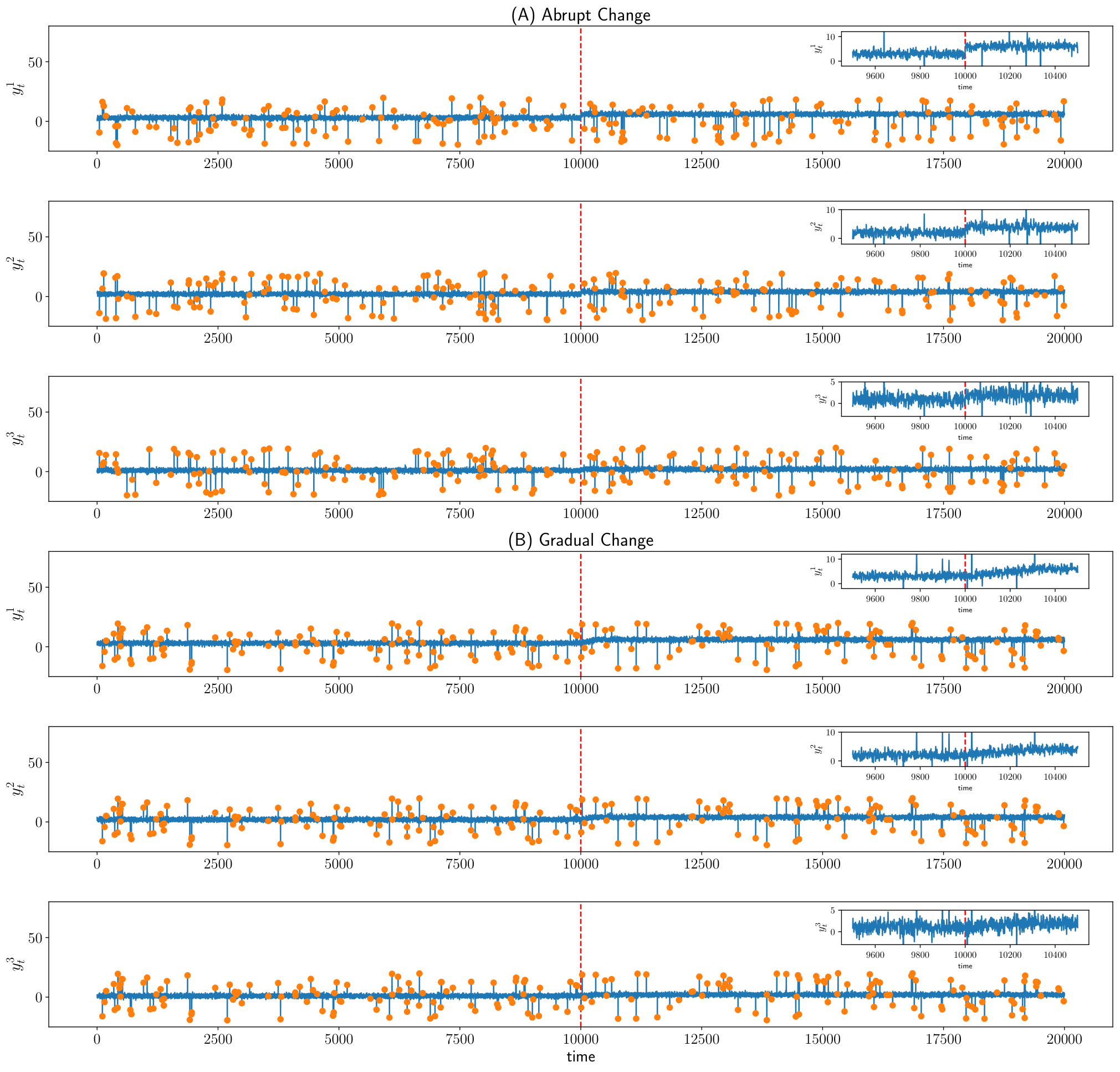
Figure 6 illustrates sample data streams with abrupt and gradual changes. Each data point $y_{t}=(y_{t}^{1},y_{t}^{2},y_{t}^{3})^{\top}$ is drawn from Equation (61) and (65) for abrupt and gradual changes, respectively. We set $\alpha=0.99$ and $U=20$ . The data points drawn from $f_{2}$ are marked with circles, and we observe that most of the data points drawn from $f_{2}$ deviate from the ones drawn from $f_{1}$ .

5.2.2 Methods for Comparison

We compared the performance of SRA with those of rival algorithms described in Section 5.1.2: iEM (Neal and Hinton 1999), sEM (Cappé and Moulines 2009), ADWIN (Bifet and Gavaldá 2007), KSWIN (Raab et al. 2020), and PH (Page 1954).

5.2.3 Evaluation metrics

We used MSE and AUC as we did in Section 5.1.3. Because ADWIN, KSWIN, and PH are designed for one-dimensional data streams, we calculated the change scores for each variable for these algorithms and then selected the variable that provided the best score.

5.2.4 Result: Comparison with other algorithms

We compared the performance of SRA with those of rival algorithms. We chose the hyperparameters with $S_{\mathrm{eval}}$ defined in Equation (56) for each algorithm as follows: $\gamma\in\{1$ , $3$ , $5$ , $7$ , $10$ , $15\}$ , $\beta\in\{0.1$ , $0.5$ , $1\}$ , and $M\in\{1$ , $5$ , $10\}$ for SRA, $r_{\mathrm{SDEM}}\in\{0.0001$ , $0.001$ , $0.005$ , $0.01\}$ for SDEM, $r_{\mathrm{sEM}}\in\{0.001$ , $0.003$ , $0.005\}$ for sEM, $\delta_{\mathrm{ADWIN}}\in\{0.001$ , $0.002$ , $0.005$ , $0.01$ , $0.02$ , $0.05$ , $0.1$ , $0.2$ , $0.5\}$ for ADWIN, $\alpha_{\mathrm{KSWIN}}\in\{0.001$ , $0.005$ , $0.01\}$ , $w_{\mathrm{KSWIN}}\in\{10$ , $20\}$ , and $r_{\mathrm{KSWIN}}\in\{10$ , $15\}$ for KSWIN, and $\delta_{\mathrm{PH}}\in\{0.001$ , $0.01$ , $0.1$ , $1$ , $10\}$ for PH.

We first evaluated SRA and the other algorithms with MSE. We generated 10 data streams according to (57) with $\alpha=0.99$ and $U=20$ using Equation (61) and (65) for abrupt and gradual changes, respectively.

Table 3 shows the average MSEs $S_{\mathrm{bc}}$ , $S_{\mathrm{ac}}$ , and $S_{\mathrm{tot}}$ for each algorithm. The hyperparamters were chosen as follows: $(\gamma$ , $\beta$ , $M)=(7$ , $0.5$ , $5)$ for SRA, $r_{\mathrm{SDEM}}=0.001$ for SDEM, $r_{\mathrm{sEM}}=0.001$ for sEM. SRA was superior to other algorithms for the time periods after the change point and before it. This result indicates that SRA has higher robustness and adaptivity than other algorithms.

Table 3: Average MSEs on the multivariate synthetic datasets.

(a) Abrupt Change

	$S_{\mathrm{bc}}$	$S_{\mathrm{ac}}$	$S_{\mathrm{tot}}$
SRA	$\mathbf{0.026\pm 0.002}$	$\mathbf{0.029\pm 0.001}$	$\mathbf{0.026\pm 0.002}$
SDEM	$1.437\pm 0.002$	$5.812\pm 0.005$	$3.894\pm 0.003$
iEM	$1.473\pm 0.001$	$5.836\pm 0.001$	$3.527\pm 0.001$
sEM	$1.399\pm 0.002$	$5.876\pm 0.003$	$3.684\pm 0.002$

(b) Gradual Change

	$S_{\mathrm{bc}}$	$S_{\mathrm{ac}}$	$S_{\mathrm{tot}}$
SRA	$\mathbf{0.016\pm 0.002}$	$\mathbf{0.007\pm 0.001}$	$\mathbf{0.003\pm 0.000}$
SDEM	$2.832\pm 0.810$	$7.018\pm 2.653$	$2.763\pm 0.793$
iEM	$0.659\pm 0.596$	$2.675\pm 1.513$	$1.514\pm 1.029$
sEM	$0.083\pm 0.007$	$0.877\pm 0.025$	$0.859\pm 0.019$

Next, we evaluated each algorithm with AUC. Table 4 shows the average AUCs for each algorithm. SRA was superior to other algorithms. The hyperparametes were chosen as follows: (i) Abrupt change: $(\gamma$ , $\beta$ , $M)=(7$ , $0.5$ , $5)$ for SRA, $r_{\mathrm{SDEM}}=0.005$ for SDEM, $r_{\mathrm{sEM}}=0.005$ for sEM, $\delta_{\mathrm{ADWIN}}=0.5$ for ADWIN, $(\alpha_{\mathrm{KSWIN}}$ , $w_{\mathrm{KSWIN}}$ , $r_{\mathrm{KSWIN}})=(0.005$ , $10$ , $15)$ for KSWIN, and $\delta_{\mathrm{PH}}=50$ for PH. (ii) Gradual change: $(\gamma$ , $\beta$ , $M)=(3$ , $0.5$ , $5)$ for SRA, $r_{\mathrm{SDEM}}=0.001$ for SDEM, $r_{\mathrm{sEM}}=0.001$ for sEM, $\delta_{\mathrm{ADWIN}}=0.5$ for ADWIN, $(\alpha_{\mathrm{KSWIN}}$ , $w_{\mathrm{KSWIN}})=(0.005$ , $10)$ for KSWIN, and $\delta_{\mathrm{PH}}=1$ for PH.

Table 4: Average AUCs on the synthetic multivariate datasets.

	Abrupt Change	Gradual Change
SRA	$\mathbf{0.753\pm 0.015}$	$\mathbf{0.721\pm 0.019}$
SDEM	$0.551\pm 0.009$	$0.532\pm 0.051$
iEM	$0.542\pm 0.008$	$0.357\pm 0.028$
sEM	$0.612\pm 0.091$	$0.527\pm 0.089$
ADWIN	$0.500\pm 0.000$	$0.500\pm 0.000$
KSWIN	$0.538\pm 0.052$	$0.515\pm 0.062$
PH	$0.482\pm 0.183$	$0.459\pm 0.139$

In summary, SRA is superior to other algorithms in terms of accuracy in detecting changes for both three-dimensional datasets with abrupt and gradual changes. Therefore, we conclude that SRA has higher robustness adaptivity than other algorithms for multivariate data streams.

5.3 Real dataset: Change detection

We applied SRA to the Well-log dataset (Ruanaidh et al. 1996) and the SKoltech Anomaly Benchmark (SKAB) dataset (Katser and Kozitsin 2020). The Well-log dataset is composed of a one-dimensional sequence, and the SKAB dataset is composed of eight-dimensional sequences.

5.3.1 Well-log dataset

The Well-log dataset is a one-dimensional data stream consisting of 4050 nuclear magnetic resonance measurements during the drilling of a well. Since it was first studied (Ruanaidh et al. 1996), it has become a benchmark dataset for univariate change detection. Although this dataset has been used in several studies (e.g., (Adams and MacKay 2007; Levy-leduc and Harchaoui 2008; Ruggieri and Antonellis 2016; Fearnhead and Rigaill 2019)), the outliers have often been removed before change detection, with the exception of only a few studies (e.g., (Fearnhead and Rigaill 2019)).

We applied SRA to the Well-log dataset for change detection. This dataset is available at https://github.com/alan-turing-institute/rbocpdms/. Figure 7 shows the annotated change points proposed by (Burg and Williams 2020). There are five sets of annotated changes, each provided by an annotator:

•

Annotation 1: $t=1069$ , $1525$ , $1681$ , $1861$ , $2053$ , $2407$ , $2473$ , $2527$ , $2587$ , $2767$ , $2779$ .
•

Annotation 2: $t=1069$ , $1525$ , $1681$ , $1867$ , $2053$ , $2407$ , $2467$ , $2527$ , $2587$ .
•

Annotation 3: $t=1069$ , $1525$ , $1687$ , $1867$ , $2053$ , $2407$ , $2473$ , $2527$ , $2587$ .
•

Annotation 4: $t=1057$ , $2797$ .
•

Annotation 5: $t=19$ , $1069$ , $1525$ , $1681$ , $1861$ , $2059$ , $2407$ , $2467$ , $2527$ , $2587$ , $2767$ , $2779$ , $3121$ , $3151$ , $3715$ , $3853$ , $3961$ .

Figure 7: Plot of the data stream and five sets of annotations of the change points for the Well-log dataset (Burg and Williams 2020). The red dashed lines indicate change points.

We used the first 1550 data points as the training dataset and the remaining points as the test dataset. We chose SDEM (Yamanishi et al. 2004), iEM (Neal and Hinton 1999), sEM (Cappé and Moulines 2009), ADWIN (Bifet and Gavaldá 2007), KSWIN (Raab et al. 2020), and PH (Page 1954) for comparison. SDEM, iEM, and sEM are online learning algorithms, and we employed the univariate normal distribution for these algorithms. ADWIN, KSWIN, and PH are concept drift detection algorithms. We calculated the change score $s_{t}$ for each algorithm in the same way as in Section 5.1.3.

We chose the hyperparameters of each algorithm with AUC scores between $t_{\mathrm{start}}=20$ and $t_{\mathrm{end}}=1550$ : the hyperparameters of SRA were chosen among $\gamma\in\{2\times 10^{6}$ , $3\times 10^{6}$ , $4\times 10^{6}\}$ , $\beta=(d_{0}+1)/L(1-\alpha)\in\{0.01\gamma$ , $0.03\gamma$ , $0.05\gamma\}$ , and $M\in\{\gamma$ , $2\gamma$ , $3\gamma\}$ , and those of SDEM and sEM were chosen among $r_{\mathrm{SDEM}},r_{\mathrm{sEM}}\in\{0.001$ , $0.003$ , $0.005$ , $0.01$ , $0.03$ , $0.05$ , $0.1\}$ . In contrast, the hyperparameters of the concept drift detection algorithms were chosen as follows: for ADWIN, $\delta_{\mathrm{ADWIN}}\in\{0.001$ , $0.002$ , $0.005$ , $0.01$ , $0.02$ , $0.05$ , $0.1$ , $0.2$ , $0.5\}$ , $\alpha_{\mathrm{KSWIN}}\in\{0.001$ , $0.005$ , $0.01\}$ , $w_{\mathrm{KSWIN}}\in\{10$ , $20\}$ , and $r_{\mathrm{KSWIN}}\in\{10$ , $15\}$ for KSWIN, and $\delta_{\mathrm{PH}}\in\{0.001$ , $0.01$ , $0.1$ , $1$ , $10\}$ for PH. We initialized each parameter or sufficient statistics of each algorithm 10 times and selected the combination that provided the best performance on average. To initialize the parameter or sufficient statistics, we drew 20 initial points from the uniform distribution with a range of $[\min(y_{20}^{40}),\max(y_{20}^{40})]$ , where $y_{20}^{40}=y_{20}\dots y_{40}$ is the sequence between $t=20$ and $t=40$ .

We applied each algorithm and calculated the AUC scores on the test dataset after the parameters were determined on the training dataset. Figure 8 displays the ROC curves on the test dataset with the algorithms and annotations. We observe that: (i) When the false alarm rate is low, SRA is not better than iEM but is overwhelmingly better than the other algorithms when the false alarm rate is over $0.1$ for Annotation 1, 2, 3, and between $0.1$ and $0.6$ for Annotation 5. (ii) SRA is almost as good as sEM for Annotation 4. We infer that (ii) is due to Annotation 4 having only two change points, and that SRA and sEM detected all the change points in a similar way.

Then, we calculated the AUC scores. Table 5 displays the AUCs for the algorithms. Because the estimated AUCs were the same for all the algorithms except SDEM, the most of standard deviations were zero. The ROC curves and AUCs were calculated in the same way as in Section 5.1.3. We observe that SRA is superior to other algorithms for each annotation. The best combinations of hyperparameters were chosen as follows: for SRA, $(\gamma,\beta,M)=(2\times 10^{6},2\times 10^{4},4\times 10^{6})$ , $(3\times 10^{6},3\times 10^{4},6\times 10^{6})$ , $(4\times 10^{6},4\times 10^{4},8\times 10^{6})$ for Annotation 1, 2, and 3, $(\gamma,\beta,M)=(3\times 10^{6},3\times 10^{4},12\times 10^{6})$ , $(2\times 10^{6},2\times 10^{4},8\times 10^{6})$ , $(4\times 10^{6},4\times 10^{4},16\times 10^{6})$ for Annotation 4, and $(\gamma,\beta,M)=(2\times 10^{6},2\times 10^{4},4\times 10^{6})$ , $(3\times 10^{6},3\times 10^{4},6\times 10^{6})$ , $(4\times 10^{6},4\times 10^{4},8\times 10^{6})$ for Annotation 5. For SDEM, $r_{\mathrm{SDEM}}=0.05$ for all the annotations. For sEM, $r_{\mathrm{sEM}}=0.003$ (Annotation 1, 2, and 3) $r_{\mathrm{sEM}}=0.005$ (Annotation 4), and $r_{\mathrm{sEM}}=0.05$ (Annotation 5). For ADWIN, $\delta_{\mathrm{ADWIN}}=0.05$ for all the annotations. For KSWIN, $(\alpha_{\mathrm{KSWIN}}$ , $w_{\mathrm{KSWIN}}$ , $r_{\mathrm{KSWIN}})=(0.005$ , $30$ , $15)$ for Annotation 1, 2, $(0.005$ , $30$ , $10)$ for Annotation 3, $(0.001$ , $30$ , $15)$ for Annotation 4, and $(0.001$ , $30$ , $10)$ for Annotation 5. For PH, $\delta_{\mathrm{PH}}=1$ for all the annotations.

Figure 8: ROC curves on the Well-log dataset for SRA, SDEM, iEM, sEM, and ADWIN.

Table 5: AUC scores on the test dataset of the Well-log dataset.

	Annotation 1	Annotation 2	Annotation 3	Annotation 4	Annotation 5
SRA	$\mathbf{0.802\pm 0.000}$	$\mathbf{0.771\pm 0.000}$	$\mathbf{0.772\pm 0.000}$	$\mathbf{0.700\pm 0.000}$	$\mathbf{0.708\pm 0.000}$
SDEM	$0.629\pm 0.003$	$0.606\pm 0.006$	$0.608\pm 0.006$	$0.673\pm 0.008$	$0.672\pm 0.005$
iEM	$0.535\pm 0.000$	$0.553\pm 0.000$	$0.546\pm 0.000$	$0.538\pm 0.000$	$0.578\pm 0.000$
sEM	$0.779\pm 0.000$	$0.747\pm 0.000$	$0.747\pm 0.000$	$0.699\pm 0.000$	$0.579\pm 0.000$
ADWIN	$0.503\pm 0.000$	$0.502\pm 0.000$	$0.502\pm 0.000$	$0.502\pm 0.000$	$0.501\pm 0.000$
KSWIN	$0.486\pm 0.000$	$0.525\pm 0.000$	$0.475\pm 0.000$	$0.415\pm 0.000$	$0.513\pm 0.000$
PH	$0.510\pm 0.000$	$0.492\pm 0.000$	$0.490\pm 0.000$	$0.549\pm 0.000$	$0.527\pm 0.000$

We further investigated how well each algorithm estimated the change scores. We chose SRA, SDEM, iEM, and sEM because we could estimate the parameters for these online learning algorithms. Figure 9 displays the estimated mean in the left panel and change scores in the right panel, respectively. The red dashed lines indicate the change points for Annotation 2. The hyperparameters were set as the best combinations for each algorithm for Annotation 2: $r_{\mathrm{SDEM}}=0.05$ for SDEM, $r_{\mathrm{sEM}}=0.003$ for sEM, and $(\gamma$ , $M$ , $\beta)=(2\times 10^{4}$ , $4\times 10^{4}$ , $2\times 10^{2})$ ( $\rho=0.0039$ ) for SRA. As for the robustness and adaptivity, we observe the following points from the left panel of Figure 9:

•

SRA and sEM were robust to changes.
•

SDEM was adaptive to changes in the underlying data generating mechanism. Therefore, it was overfitted.
•

iEM was robust (and not adaptive) to changes.

As for the estimated change scores, we also observe from the right panel of Figure 9 that SDEM, iEM, and sEM were prone to outliers, in particular after $t=2500$ , whereas SRA was less influenced by outliers. On the other hand, for time points between $t=300$ and $t=1100$ , it is hard to distinguish between the outliers and essential changes based only on the change scores estimated with SRA.

Figure 9: Estimated mean

\hat{\mu}_{t}

and change scores for the Well-log dataset. The left and right panels display the estimated mean and change score for each algorithm, respectively. The red dashed lines indicate the change points for Annotation 2.

5.3.2 SKAB dataset

The SKAB dataset is composed of 34 eight-dimensional data streams (Katser and Kozitsin 2020), which were collected from a testbed of a water circulation system. This dataset is available at https://www.kaggle.com/dsv/1693952.

Anomalies and change points are annotated for each sequence. Here, the anomalies and change points refer to time points at which the machines operated abnormally and time points at which the mode of abnormality changed, respectively.

We chose 16 sequences obtained from the experiments, where the valve at the outlet of the flow from the pump was closed. Figure 10 shows a sample sequence of the SKAB dataset. The machine started to change gradually at $t=574$ from normal mode and reached abnormal mode at $t=632$ (the first span indicated by a green color). In contrast, the machine started to change gradually at $t=919$ from abnormal mode and reached normal mode at $t=978$ (the second span indicated by green color). The machine remained in abnormal mode between $t=633$ and $t=918$ (the span indicated by red). Therefore, we defined the change points used for evaluating SRA and the other algorithms at $t=574$ and $919$ (the vertical red dashed lines). We clearly observe that there are anomaly points of $y_{3}$ at $t=338$ and $t=495$ , and $y_{7}$ at $t=495$ .

Figure 10: A sample sequence of the SKAB dataset. The machine changed gradually from normal mode at

t=574

and reached abnormal mode at

t=632

(the first span indicated by a light green color). Next, the machine remained at abnormal mode between

t=633

and

918

(the span indicated by the light red color). Finally, the machine changed gradually from abnormal mode at

t=919

and reached normal mode at

t=978

(the second span indicated by a light green color). Therefore, we annotated the change points at

t=745

and

924

, as shown with red dashed lines.

We compared the performance of SRA with those of SDEM (Yamanishi et al. 2004), iEM (Neal and Hinton 1999), sEM (Cappé and Moulines 2009), ADWIN (Bifet and Gavaldá 2007), KSWIN (Raab et al. 2020), and PH (Page 1954). We calculated the change score $s_{t}$ for each algorithm in the same way as in Section 5.1.3.

We chose the hyperparameters of each algorithm with AUC scores between $t=20$ and the end time point. The hyperparameters were selected as follows: for SRA, $\gamma\in\{80$ , $90$ , $100\}$ , $\beta\in\{1$ , $5$ , $10\}$ , and $M\in\{10000$ , $20000$ , $30000\}$ . For SDEM, $r_{\mathrm{SDEM}}\in\{0.01$ , $0.03$ , $0.05$ , $0.1$ , $0.3$ , $0.5\}$ . For sEM, $r_{\mathrm{sEM}}\in\{0.01$ , $0.03$ , $0.05$ , $0.1$ , $0.3$ , $0.5\}$ . For ADWIN, $\delta_{\mathrm{ADWIN}}\in\{0.001$ , $0.002$ , $0.005$ , $0.01$ , $0.02$ , $0.05$ , $0.1$ , $0.2$ , $0.5\}$ . For KSWIN, $\alpha_{\mathrm{KSWIN}}\in\{0.001$ , $0.005$ , $0.01$ , $w_{\mathrm{KSWIN}}\in\{20$ , $30\}$ , and $r_{\mathrm{KSWIN}}\in\{10$ , $15\}$ . For PH, $\delta_{\mathrm{PH}}\in\{0.01$ , $0.05$ , $0.1$ , $0.5$ , $1$ , $5$ , $10\}$ . For ADWIN, KSWIN, and PH, we calculated AUCs for each univariate sequence and selected the one which gave the best AUC score. We set the number of clusters $K=1$ for SRA, SDEM, iEM, and sEM.

We used eight sequences labeled odd indexes as the training dataset and the remaining eight sequences labeled even indexes as the test dataset. We converted each variable $y_{t}^{i}\leftarrow(y_{t}^{i}-\hat{\mu}^{i})/\hat{\sigma}^{i}$ ( $i=1,\dots,8$ ), where $\hat{\mu}^{i}$ and $\hat{\sigma}^{i}$ were the estimated mean and standard deviation using the first 100 data points. We initialized the parameters of SRA, SDEM, iEM, and sEM using data points between $t=20$ and $40$ . We repeated this procedure 5 times.

Table 6 shows the AUCs on the test dataset for all the algorithms. We set the maximum tolerance delay $T_{\mathrm{b}}=20$ and $50$ in Equation (53). We observe that SRA is superior to the other algorithms for both the values of $T_{\mathrm{b}}$ . The best combinations of hyperparameters were selected as follows: $(\gamma$ , $\beta$ , $M)=(80$ , $5$ , $50000)$ for SRA, $r_{\mathrm{SDEM}}=0.03$ for SDEM, $r_{\mathrm{sEM}}=0.03$ for sEM, $\delta_{\mathrm{ADWIN}}=0.1$ and the fifth variable for ADWIN, $(\alpha_{\mathrm{KSWIN}}$ , $w_{\mathrm{KSWIN}}$ , $r_{\mathrm{KSWIN}})=(0.005$ , $30$ , $10)$ and the eighth variable for KSWIN, and $\delta_{\mathrm{PH}}=10$ and the third variable for PH.

Table 6: AUC scores on the test dataset of the SKAB dataset.

T_{\mathrm{b}}

is the maximum tolerant delay defined in Equation (53).

	$T_{\mathrm{b}}=20$	$T_{\mathrm{b}}=50$
SRA	$\mathbf{0.551\pm 0.043}$	$\mathbf{0.580\pm 0.085}$
SDEM	$0.543\pm 0.135$	$0.565\pm 0.119$
iEM	$0.529\pm 0.125$	$0.544\pm 0.078$
sEM	$0.537\pm 0.078$	$0.498\pm 0.055$
ADWIN	$0.505\pm 0.012$	$0.512\pm 0.005$
KSWIN	$0.536\pm 0.085$	$0.459\pm 0.059$
PH	$0.422\pm 0.116$	$0.518\pm 0.166$

In summary, SRA outperformed the other online learning algorithms and concept drift detection algorithms for a univariate data stream with abrupt changes as well as multivariate data streams with gradual changes. Although this empirical study shows the performance of SRA, it remains future work to present theoretical analysis of SRA for data streams with gradual changes beyond the one presented in Section 4.

5.4 Real dataset: Anomaly detection

We applied SRA to anomaly detection in two real datasets: the SMTP and THYROID dataset. Both datasets are publicly available at http://odds.cs.stonybrook.edu/smtp-kddcup99-dataset. Table 7 summarizes each dataset.

Figure 11 shows the data stream of the SMTP dataset. We observe that: (i) Anomalies are concentrated around $t=15000$ : $t=14692$ , $14742$ , $14789$ , $14833$ , $14888$ , $14967$ , $15016$ , $15043$ , $15099$ , $15165$ , $15221$ , $15283$ , and $15366$ . (ii) Although we see that all the variables deviate from these normal values at anomaly points around $t=15000$ , it is not the case for anomalies after $t=49000$ . Therefore, the mechanism of anomaly is also thought of as complicated.

Table 7: Summary of the real datasets for anomaly detection.

	SMTP	THYROID
Sequence length	95156	3772
Number of attributes	3	6
Number of outliers	30	93
Ratio of outliers	0.03%	2.5%

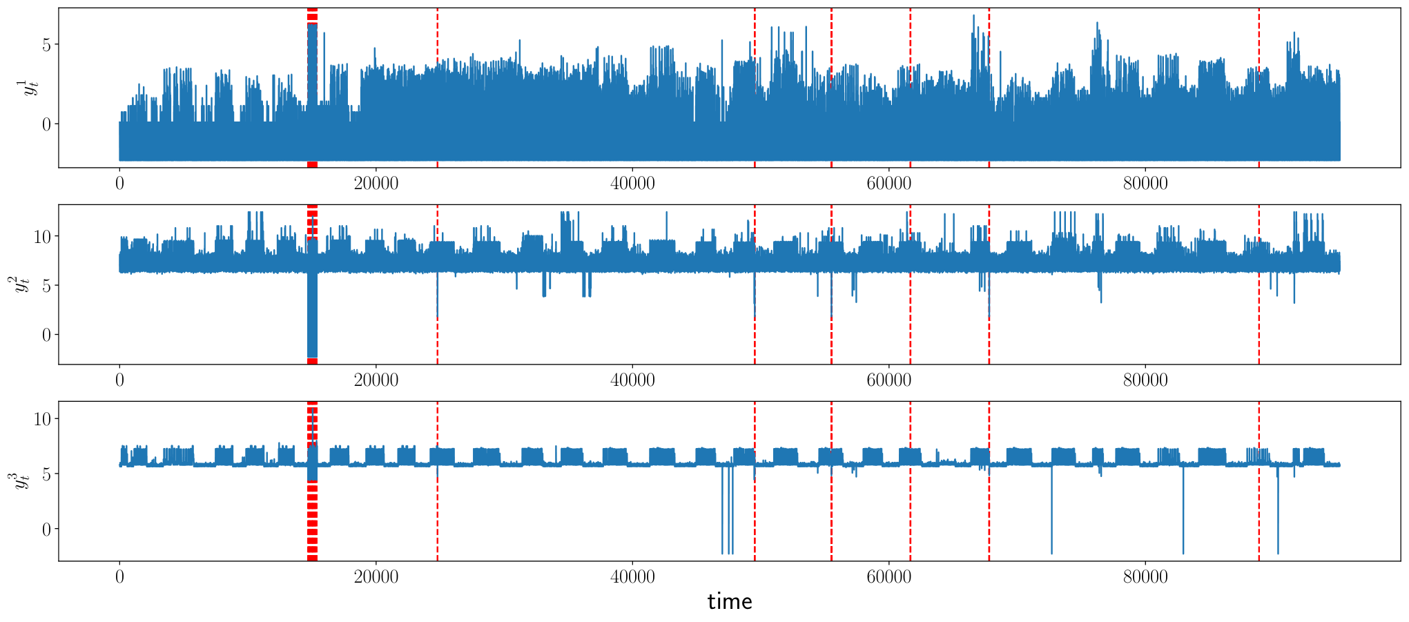
Figure 11 shows the data stream of the THYROID dataset. We observe that some anomalies are visible. For example, the second variable $y_{t}^{2}$ deviates from normal values at $t=518$ , $520$ , $640$ , $687$ , $861$ , and $965$ . However, this observation is not applicable to all the anomalies. Therefore, the mechanism of anomaly is thought of as complicated.

Figure 12: Plot of THYROID dataset. The red dashed lines indicate anomalies.

We used the first 40000 and 2000 data points as the training dataset for the SMTP and THYROID dataset, respectively, and the remaining data points as the test dataset. We chose SDEM (Yamanishi et al. 2004), iEM (Neal and Hinton 1999), sEM (Cappé and Moulines 2009), ADWIN (Bifet and Gavaldá 2007), KSWIN (Raab et al. 2020), and PH (Page 1954) for comparison. For SRA, SDEM, iEM, and sEM, each algorithm used GMM, and the number of components was selected among $K\in\{1,2,3\}$ .

We calculated the anomaly score as $s_{t}\mathrel{\overset{\makebox[0.0pt]{\mbox{\tiny def}}}{=}}-\log{f(x_{t};\hat{\theta}_{t-1})}$ , where $\hat{\theta}_{t-1}$ is the parameter estimated at $t-1$ . Then, we chose the best combinations with the AUC scores between $t=10000$ and $t=40000$ for SMTP and between $t=1000$ and $t=2000$ for THYROID. The AUC score was calculated based on the anomaly scores, and the ground truth labels associated with each data point, which indicate whether a data point is an anomaly or not. Note that the AUC score here is different from the one in Section 5.3.

For both training datasets, we chose the hyperparameters among $\gamma\in\{5,10,15\}$ , $\beta=(d_{0}+1)/L(1-\alpha)\in\{0.1,0.5,1\}$ , and $M\in\{1,5,10\}$ for SRA, $r_{\mathrm{SDEM}}\in\{0.1,0.3,0.5\}$ for SMTP and $r_{\mathrm{SDEM}}\in\{0.01,0.03,0.05,0.1\}$ for THYROID, $r_{\mathrm{sEM}}\in\{0.01,0.03,0.05,0.1\}$ for SMTP and $r_{\mathrm{sEM}}\in\{0.0001,0.001,0.005\}$ for THYROID, $\delta_{\mathrm{ADWIN}}\in\{0.001$ , $0.002$ , $0.005$ , $0.01$ , $0.02$ , $0.05$ , $0.1$ , $0.2$ , $0.5\}$ , $\alpha_{\mathrm{KSWIN}}\in\{0.001$ , $0.005$ , $0.01\}$ , $w_{\mathrm{KSWIN}}\in\{0.001$ , $0.005$ , $0.01\}$ , $r_{\mathrm{KSWIN}}\in\{10$ , $15\}$ , and $\delta_{\mathrm{PH}}\in\{0.01$ , $0.05$ , $0.1$ , $0.5$ , $1$ , $5$ , $10\}$ .

As a result, the following parameters were chosen: for the SMTP dataset, $(\gamma$ , $\beta$ , $M$ , $K)=(10$ , $0.5$ , $5$ , $2)$ for SRA, $(r_{\mathrm{SDEM}}$ , $K)=(0.3$ , $3)$ for SDEM, $(r_{\mathrm{sEM}}$ , $K)=(0.03$ , $3)$ for sEM, $\delta_{\mathrm{ADWIN}}=0.1$ and the second variable for ADWIN, $(\alpha_{\mathrm{KSWIN}}$ , $w_{\mathrm{KSWIN}}$ , $r_{\mathrm{KSWIN}})=(0.005$ , $20$ , $10)$ and the third variable for KSWIN, and all the values of hyperparameters and the third variable for PH. For the THYROID dataset, $(\gamma$ , $\beta$ , $M$ , $K)=(10$ , $0.5$ , $5$ , $3)$ for SRA, $(r_{\mathrm{SDEM}}$ , $K)=(0.01$ , $3)$ for SDEM, $(r_{\mathrm{sEM}}$ , $K)=(0.001$ , $3)$ for sEM, all the values of the hyperparameters and the first variable for ADWIN, $(\alpha_{\mathrm{KSWIN}}$ , $w_{\mathrm{KSWIN}}$ , $r_{\mathrm{KSWIN}})=(0.005$ , $20$ , $10)$ and the third variable for KSWIN, and all the values of the hyperparameters and the second variable for PH.

To initialize the parameters or sufficient statistics, we drew 20 initial points for each algorithm. Each coordinate of the points was drawn from a uniform distribution with range set in the same way as in Section 5.3. We repeated this procedure 10 times and selected the combination of parameters that yielded the best performance on average.

Table 8 shows the AUC scores on the test datasets for SMTP and THYROID. We observe that SRA outperforms other online learning algorithms and concept drift detection algorithms in anomaly detection.

Table 8: AUC scores on the SMTP dataset and THYROID dataset.

	SMTP	THYROID
SRA	$\mathbf{0.874\pm 0.001}$	$\mathbf{0.972\pm 0.000}$
SDEM	$0.773\pm 0.000$	$0.933\pm 0.000$
iEM	$0.744\pm 0.000$	$0.935\pm 0.000$
sEM	$0.773\pm 0.000$	$0.968\pm 0.000$
ADWIN	$0.498\pm 0.000$	$0.500\pm 0.000$
KSWIN	$0.493\pm 0.051$	$0.478\pm 0.027$
PH	$0.424\pm 0.000$	$0.709\pm 0.000$

5.5 Concluding Remarks

In Section 5.1 and 5.2, we confirmed that SRA is robust to outliers and adaptive to changes, in comparison with the other online learning algorithms and concept drift detection algorithms, for both synthetic univariate and multivariate datasets with abrupt and gradual changes. SRA outperformed the other online learning algorithms with MSE. SRA also outperformed the online learning algorithms and concept drift detection algorithms with AUC. However, we also confirmed that SRA took more total time to tune hyperparameters than the other algorihms because SRA has more hyperparameters. SRA also took more time for a set of hyperparameters because SRA requires the calculation of probability densities of parametric distributions in calculating the change scores.

In Section 5.3, we confirmed that SRA also worked for real datasets in change detection. For both univariate and multivariate datasets, SRA was better than the other algorithms with AUC. We also visualized estimated parameters and change scores and concluded that SRA was excellent in both robustness and adaptivity, whereas other online learning algorithms either overfitted the changes or were not adaptive to changes.

In Section 5.4, we confirmed that SRA was also superior to the other online learning algorithms and concept drift detection algorithms in anomaly detection.

In summary, SRA is excellent in estimation of parameters, change detection, and anomaly detection, compared to the other online learning algorithms and concept drift detection algorithms. SRA has a sound theoretical background for quantitatively characterizing the tradeoff between the robustness and adaptivity. However, SRA took much more time to tune hyperparameters. Furthermore, although SRA is formulated based on datasets with abrupt changes, empirical studies show that it also works on datasets with gradual changes for both the synthetic datasets in Section 5.1.6 and real datasets in Section 5.3.2. Future work will verify the theoretical performance of SRA on datasets with gradual changes.

6 Conclusion

In this study, we quantitatively evaluate the tradeoff between the robustness and adaptivity of online learning algorithms. We proposed a novel algorithm, called SRA, to consider this tradeoff. SRA updates parameters of distribution or sufficient statistics in an online fashion, using the SA scheme (Robbins and Monro 1951). No update is done when the norm of the stochastic update exceeds the threshold. We showed the upper bound of the expectation of the mean field of the stochastic update in the SA scheme. We further explicitly derived the relation between two parameters: 1) step size of the SA scheme and 2) threshold parameter of the stochastic update. The empirical experiments for the synthetic datasets demonstrated that the dependencies on the parameters of SRA are consistent with the theoretical analysis, and that SRA is superior to previous online learning algorithms and concept drift detection algorithms. The experiments on real datasets also demonstrated that SRA is superior to other algorithms in change detection and anomaly detection.

Future work includes extension of SRA to gradual changes of parameters. Another interesting line of research lies in a theoretical analysis as well as empirical experiments in a setting where the step size is determined adaptively and reset after a change point.

References

Adams and MacKay (2007) Adams R, MacKay D (2007) Bayesian online changepoint detection. arXiv preprint arXiv:07103742
Balakrishnan et al. (2017) Balakrishnan S, Wainwright MJ, Yu B (2017) Statistical gurantees for the em algorithm: From population to sample-based analysis. The annals of statistics 45(1):77–120
Bifet and Gavaldá (2007) Bifet A, Gavaldá R (2007) Learning from time-changing data with adaptive windowing. In: 2007 SIAM international conference on data mining, pp 443–448
Bottou et al. (2018) Bottou L, Curtis FE, Nocedal J (2018) Optimization methods for large-scale machine learning. SIAM Review 60(2):223–311
Burg and Williams (2020) Burg GJJ, Williams CKI (2020) An evaluation of change point detection algorithms. arXiv preprint arXiv:200306222
Cappé and Moulines (2009) Cappé O, Moulines E (2009) On-line expectation-maximization algorithm for latent data models. J R Statist Soc B 71(3):593–613
Cejnek and Bukovsky (2018) Cejnek M, Bukovsky I (2018) Concept drift robust adaptive novelty detection for data streams. Neurocomputing 309(2):46–53
Chen et al. (2018) Chen J, Zhu J, Teh YW, , Zhang T (2018) Stochastic expectation maximization with variance reduction. In: Proceedings of Advances in Neural Information Processing (NeurIPS) 31, pp 7978–7988
Chu et al. (2004) Chu F, Wang Y, Zaniolo C (2004) An adaptive learning approach for noisy data streams. In: Proceedings of IEEE International Conference on Data Mining (ICDM), pp 351–354
Dempster et al. (1977) Dempster AP, Laird NM, Rubin DB (1977) Maximum likelihood from incomplete data via the em algorithm. Journal of the royal statistical society Series B (methodological) pp 1–38
Fawcett and Provost (1999) Fawcett T, Provost F (1999) Activity monitoring: noticing interesting changes in behavior. In: Proceedings of the Fifth ACM SIGKDD International Conference on Knowledge Discovery and Data Mining (KDD), pp 53–62
Fearnhead and Rigaill (2019) Fearnhead P, Rigaill G (2019) Changepoint detection in the presence of outliers. Journal of the American Statistical Association 114(525):169–183
Fukushima and Yamanishi (2019) Fukushima S, Yamanishi K (2019) Detecting metachanges in data streams from the viewpoint of the MDL principle. Entropy 21:1134
Fukushima and Yamanishi (2020) Fukushima S, Yamanishi K (2020) Hierarchical change detection in latent variable models. In: Proceedings of 2020 IEEE International Conference on Data Mining (ICDM), pp 1128–1133
Gama et al. (2014) Gama J, Žliobaitė I, Bifet A, Mykola P, Abdelhamid B (2014) A survey on concept drift adaptation. ACM Computing Surveys 46(4)
Ghadimi and Lan (2013) Ghadimi S, Lan G (2013) Stochastic first-and zeroth-order methods for nonconvex stochastic programming. SIAM Journal on Optimization 23(4):2341–2368
Gonçalves et al. (2014) Gonçalves PM, de Carvalho Santos SG, Barros RS, Vieira DC (2014) A comparative study on concept drift detectors. Expert Systems with Applications 41(18):8144–8156
Guo (2019) Guo W (2019) Robust adaptive online sequential extreme learning machine for predicting nonstationary data streams with outliers. Journal of algorithms and computational technology 13:1–16
Hara et al. (2019) Hara S, Nitanda A, Maehara T (2019) Data cleansing for models trained with SGD. In: Proceedings of Advances in Neural Information Processing Systems (NeurIPS) 32, pp 4213–4222
Huang et al. (2016) Huang SY, Lin JW, Tsaih RH (2016) Outlier detection in the concept drifting environment. In: Proceedings of International Joint Conference on Neural Network (IJCNN), pp 31–37
Karimi et al. (2019a) Karimi B, Lavielle M, Moulines E, Wai HT (2019a) Non-asymptotic analysis of biased stochastic approximation scheme. In: Proceedings of Conference on Learning Theory (COLT)
Karimi et al. (2019b) Karimi B, Lavielle M, Moulines E, Wai HT (2019b) On the global convergence of (fast) incremental expectation maximization methods. In: Proceedings of Advances in Neural Information Processing Systems (NeurIPS) 32, pp 2837–2847
Katser and Kozitsin (2020) Katser ID, Kozitsin VO (2020) Skoltech anomaly benchmark (SKAB). https://www.kaggle.com/dsv/1693952, accessed: 8th Sep. 2021
Lange (2016) Lange K (2016) MM Optimization Algorithms. SIAM-Society for Industrial and Applied Mathematics, USA
Lattimore and Szepesväri (2018) Lattimore T, Szepesväri C (2018) Bandit algorithms, https://tor-lattimore.com/downloads/book/book.pdf
Levy-leduc and Harchaoui (2008) Levy-leduc C, Harchaoui Z (2008) Catching change-points with lasso. In: Proceedings of Advances in Neural Information Processing Systems (NIPS), pp 617–624
Mairal (2015) Mairal J (2015) Incremental majorization-minimization optimization with application to large-scale machine learning. SIAM J Optim 25(2):829–855
Montiel et al. (2018) Montiel J, Read J, Bifet A, Abdessalem T (2018) Scikit-multiflow: A multi-output streaming framework. Journal of Machine Learning Research 19(72):1–5, URL http://jmlr.org/papers/v19/18-251.html
Neal and Hinton (1999) Neal R, Hinton G (1999) A view of the em algorithm that justifies incremental, sparse, and other variants. Learning in Graphical Models pp 355–368
Odakura (2018) Odakura M (2018) Online nonstationary robust learning and its application to anomaly detection (Bachelor thesis in The University of Tokyo)
Page (1954) Page E (1954) Continuous inspection schemes. Biometrika 41(1/2):100–115
Raab et al. (2020) Raab C, Heusinger M, Schleif FM (2020) Reactive soft prototype computing for concept drift streams. Neurocomputing 416:340–351
Robbins and Monro (1951) Robbins H, Monro S (1951) A stochastic approximation method. The Annals of Mathematical Statistics 22(3):400–407
Ruanaidh et al. (1996) Ruanaidh O, Joseph JK, Fitzgerald WJ (1996) Numerical bayesian methods applied to signal processing. Springer
Ruggieri and Antonellis (2016) Ruggieri E, Antonellis M (2016) An exact approach to Bayesian sequential change point detection. Computational Statistics and Data Analysis 97:71–86
Tsay (1988) Tsay RS (1988) Outliers, level shifts, and variance changes in time series. Journal of forecasting 7:1–20
Vershynin (2018) Vershynin R (2018) High-dimensional probability: An introduction with applications in data scaence. Cambridge University Press
Yamanishi and Miyaguchi (2016) Yamanishi K, Miyaguchi K (2016) Detecting gradual changes from data stream using MDL-change statistics. In: Proceedings of 2016 IEEE International Conference on BigData (BigData), pp 156–163
Yamanishi and Takeuchi (2002) Yamanishi K, Takeuchi J (2002) A unifying framework for detecting outliers and change points from non-stationary time series data. In: Proceedings of the eighth ACM SIGKDD international conference on Knowledge discovery and data mining (KDD), pp 676–681
Yamanishi et al. (2004) Yamanishi K, Takeuchi J, Williams G, Milne P (2004) On-line unsupervised outlier detection using finite mixtures with discounting learning algorithms. Data Mining and Knowledge Discovery 8(3):275–300

Appendix A Proofs for Section 4

In this section, we describe all the proofs for Section 4.

A.1 Proof of Lemma 1

Proof

It is easily shown that

$\displaystyle\mathbb{E}[-\langle\nabla V(\theta_{k})\|\xi_{k+1}\rangle\mid\mathcal{F}_{k}]$	$\displaystyle=\mathbb{E}[-\langle\nabla V(\theta_{k})\|G_{\theta_{k}}(Y_{k+1})-h(\theta_{k})\rangle\mid\mathcal{F}_{k}]$	(66)
	$\displaystyle=\mathbb{E}[-\langle\nabla V(\theta_{k})\|G_{\theta_{k}}(Y_{k+1})-\mathbb{E}[H_{\theta_{k}}(Y_{k+1})\mid\mathcal{F}_{k}]\rangle\mid\mathcal{F}_{k}]$	(67)
	$\displaystyle\leq[\langle\nabla V(\theta_{k})\|\mathbb{E}[\\|G_{\theta_{k}}(Y_{k+1})-H_{\theta_{k}}(Y_{k+1})\\|]\rangle\mid\mathcal{F}_{k}]$	(68)
	$\displaystyle\leq\\|\nabla V(\theta_{k})\\|\mathbb{E}[\\|G_{\theta_{k}}(Y_{k+1})-H_{\theta_{k}}(Y_{k+1})\\|\mid\mathcal{F}_{k}]$	(69)
	$\displaystyle\leq\\|\nabla V(\theta_{k})\\|\int_{0}^{\infty}P[\\|G_{\theta_{k}}(Y_{k+1})-H_{\theta_{k}}(Y_{k+1})\\|\geq z]\,\mathrm{d}z$	(70)
	$\displaystyle\leq\\|\nabla V(\theta_{k})\\|\int_{\gamma}^{\infty}P[\\|G_{\theta_{k}}(Y_{k+1})-H_{\theta_{k}}(Y_{k+1})\\|\geq z]\,\mathrm{d}z$	(71)
	$\displaystyle=\\|\nabla V(\theta_{k})\\|\int_{\gamma}^{\infty}P[\\|H_{\theta_{k}}(Y_{k+1})\\|\geq z]\,\mathrm{d}z.$	(72)

When $\mathbb{E}[\|e_{k+1}\|^{2}|\mathcal{F}_{k}]<\infty$ holds, there exists $M>0$ such that the following inequality holds:

\displaystyle P[\|H_{\theta_{k}}(Y_{k+1})\|\geq z]\leq\exp{\left(-\frac{z^{2}}{M^{2}}\right)}.

(73)

Then, we have

\displaystyle\mathbb{E}[-\langle\nabla V(\theta_{k})|\xi_{k+1}\rangle\mid\mathcal{F}_{k}]

\displaystyle\leq\|\nabla V(\theta_{k})\|\int_{\gamma}^{\infty}\exp{\left(-\frac{z^{2}}{M^{2}}\right)}\,\mathrm{d}z.

(74)

A.2 Proof of Lemma 2

Proof

First, when $Y_{k+1}\sim f(Y_{k+1};\theta_{k})$ , we have

$\displaystyle\mathbb{E}[\\|\xi_{k+1}\\|^{2}\|\mathcal{F}_{k}]$	$\displaystyle=P(\\|H_{\theta_{k}}(Y_{k+1})\\|\geq\gamma)\,\mathbb{E}[\\|h(\theta_{k})\\|^{2}\mid\mathcal{F}_{k},\\|H_{\theta_{k}}(Y_{k+1})\\|\geq\gamma]$	(75)
	$\displaystyle\quad+P(\\|H_{\theta_{k}}(Y_{k+1})\\|<\gamma)\mathbb{E}[\\|H_{\theta_{k}}(Y_{k+1})-h(\theta_{k})\\|^{2}\mid\mathcal{F}_{k},\\|H_{\theta_{k}}(Y_{k+1})\\|<\gamma]$	(76)
	$\displaystyle\leq P(\\|H_{\theta_{k}}(Y_{k+1})\\|\geq\gamma)\,\mathbb{E}[\\|h(\theta_{k})\\|^{2}\mid\mathcal{F}_{k}]$	(77)
	$\displaystyle\quad+P(\\|H_{\theta_{k}}(Y_{k+1})\\|<\gamma)\,(\sigma_{0}^{2}+\sigma_{1}^{2}\mathbb{E}[\\|h(\theta_{k})\\|^{2}\mid\mathcal{F}_{k}])$	(78)
	$\displaystyle\leq\sigma_{0}^{2}+(\sigma_{1}^{2}+1)\mathbb{E}[\\|h(\theta_{k})\\|^{2}\mid\mathcal{F}_{k}].$	(79)

Next, when $Y_{k+1}\sim f_{\mathrm{noise}}$ , we have

\displaystyle\mathbb{E}[\|\xi_{k+1}\|^{2}\mid\mathcal{F}_{k}]\leq\min(dU^{2},\gamma^{2}).

(80)

Then, we have

\displaystyle\mathbb{E}[\|\xi_{k+1}\|^{2}\mid\mathcal{F}_{k}]

\displaystyle\leq\alpha\left\{\sigma_{0}^{2}+(\sigma_{1}^{2}+1)\mathbb{E}[\|h(\theta_{k})\|^{2}|\mathcal{F}_{k}]\right\}+(1-\alpha)\min(dU^{2},\gamma^{2}).

(81)

A.3 Proof of Theorem 4.1

Proof

As the Lyapunov function $V(\theta)$ is $L$ -smooth, we obtain

$\displaystyle V(\theta_{k+1})$	$\displaystyle\leq V(\theta_{k})-\rho_{k+1}\langle\nabla V(\theta_{k})\|G_{\theta_{k}}(Y_{k+1})\rangle+\frac{L\rho_{k+1}^{2}}{2}\\|G_{\theta_{k}}(Y_{k+1})\\|^{2}$	(82)
	$\displaystyle=V(\theta_{k})-\rho_{k+1}\langle\nabla V(\theta_{k})\|h({\theta_{k}})+\xi_{k+1}\rangle$	(83)
	$\displaystyle\quad+\frac{L\rho_{k+1}^{2}}{2}(\\|h(\theta_{k})\\|^{2}+2\langle h(\theta_{k})\|\xi_{k+1}\rangle+\\|\xi_{k+1}\\|^{2})$	(84)
	$\displaystyle\leq V(\theta_{k})-\rho_{k+1}\langle\nabla V(\theta_{k})\|h(\theta_{k})+\xi_{k+1}\rangle+L\rho_{k+1}^{2}(\\|h(\theta_{k})\\|^{2}+\\|\xi_{k+1}\\|^{2}).$	(85)

The equality in the last equation in Equation (85) holds when $\xi_{k+1}=h(\theta_{k})$ . Rearranging terms yields

\displaystyle\rho_{k+1}\langle\nabla V(\theta_{k})|h(\theta_{k})\rangle

\displaystyle\leq V(\theta_{k})-V(\theta_{k+1})-\rho_{k+1}\langle\nabla V(\theta_{k})|\xi_{k+1}\rangle+L\rho_{k+1}^{2}(\|h(\theta_{k})\|^{2}+\|\xi_{k+1}\|^{2}).

(86)

As $\langle\nabla V(\theta_{k})|h(\theta_{k})\rangle\geq\frac{1}{c_{1}}(\|h(\theta_{k})\|^{2}-c_{0})$ , we get

$\displaystyle\frac{\rho_{k+1}}{c_{1}}(\\|h(\theta_{k})\\|^{2}-c_{0})$	$\displaystyle\leq V(\theta_{k})-V(\theta_{k+1})$	(87)
	$\displaystyle\quad-\rho_{k+1}\langle\nabla V(\theta_{k})\|\xi_{k+1}\rangle+L\rho_{k+1}^{2}(\\|h(\theta_{k})\\|^{2}+\\|\xi_{k+1}\\|^{2})$	(88)
$\displaystyle\Longleftrightarrow\frac{\rho_{k+1}}{c_{1}}(1-c_{1}L\rho_{k+1})\\|h(\theta_{k})\\|^{2}$	$\displaystyle\leq\frac{c_{0}}{c_{1}}\rho_{k+1}+V(\theta_{k})-V(\theta_{k+1})$	(89)
	$\displaystyle\quad-\rho_{k+1}\langle\nabla V(\theta_{k})\|\xi_{k+1}\rangle+L\rho_{k+1}^{2}\\|\xi_{k+1}\\|^{2}.$	(90)

Let us sum up both sides in Equation (90) from $k=0$ to $k=n$ and rearrange terms, then we get

	$\displaystyle\sum_{k=0}^{n}\frac{\rho_{k+1}}{c_{1}}(1-c_{1}L\rho_{k+1})\\|h(\theta_{k})\\|^{2}$	$\displaystyle\leq\frac{c_{0}}{c_{1}}\sum_{k=0}^{n}\rho_{k+1}+V(\theta_{0})-V(\theta_{n+1})$		(91)
		$\displaystyle\quad-\sum_{k=0}^{n}\rho_{k+1}\langle\nabla V(\theta_{k})\|\xi_{k+1}\rangle+L\sum_{k=0}^{n}\rho_{k+1}^{2}\\|\xi_{k+1}\\|^{2}.$		(92)

Taking expectation in both sides of Equation (92) gives

$\displaystyle\sum_{k=0}^{n}\frac{\rho_{k+1}}{c_{1}}(1-c_{1}L\rho_{k+1})\mathbb{E}[\\|h(\theta_{k})\\|^{2}\|\mathcal{F}_{k}]$	$\displaystyle\leq\frac{c_{0}}{c_{1}}\sum_{k=0}^{n}\rho_{k+1}+V_{0,n}$	(93)
	$\displaystyle\quad-\sum_{k=0}^{n}\rho_{k+1}\mathbb{E}[\langle\nabla V(\theta_{k})\|\xi_{k+1}\rangle\mid\mathcal{F}_{k}]$	(94)
	$\displaystyle\quad+L\sum_{k=0}^{n}\rho_{k+1}^{2}\mathbb{E}[\\|\xi_{k+1}\\|^{2}\mid\mathcal{F}_{k}].$	(95)

Substituting Equation (26) and (28) to the second and third term in Equation (95), we have the following inequality:

		$\displaystyle\sum_{k=0}^{n}\frac{\rho_{k+1}}{c_{1}}(1-c_{1}L\rho_{k+1})\mathbb{E}[\\|h(\theta_{k})\\|^{2}\|\mathcal{F}_{k}]$		(96)
		$\displaystyle\leq\frac{c_{0}}{c_{1}}\sum_{k=0}^{n}\rho_{k+1}+V_{0,n}+\sum_{k=0}^{n}\rho_{k}\\|\nabla V(\theta_{k})\\|\int_{\gamma}^{\infty}\exp{\left(-\frac{z^{2}}{M^{2}}\right)}\,\mathrm{d}z$		(97)
		$\displaystyle\quad+L\sum_{k=0}^{n}\rho_{k+1}^{2}\left\{\alpha(\sigma_{0}^{2}+(\sigma_{1}^{2}+1)\mathbb{E}[\\|h(\theta_{k})\\|^{2}\mid\mathcal{F}_{k}])+(1-\alpha)\min(dU^{2},\gamma^{2})\right\}$		(98)
		$\displaystyle\leq\frac{c_{0}}{c_{1}}\sum_{k=0}^{n}\rho_{k+1}+V_{0,n}+\sum_{k=0}^{n}\rho_{k}(d_{0}+d_{1}\\|h(\theta_{k})\\|)\int_{\gamma}^{\infty}\exp{\left(-\frac{z^{2}}{M^{2}}\right)}\,\mathrm{d}z$		(99)
		$\displaystyle\quad+L\sum_{k=0}^{n}\rho_{k+1}^{2}\left\{\alpha(\sigma_{0}^{2}+(\sigma_{1}^{2}+1)\mathbb{E}[\\|h(\theta_{k})\\|^{2}\mid\mathcal{F}_{k}])+(1-\alpha)\min(dU^{2},\gamma^{2})\right\}$		(100)
		$\displaystyle\leq\frac{c_{0}}{c_{1}}\sum_{k=0}^{n}\rho_{k+1}+V_{0,n}+\sum_{k=0}^{n}\rho_{k+1}\left(d_{0}+d_{1}(\\|h(\theta_{k})\\|^{2}+1)\right)\int_{\gamma}^{\infty}\exp{\left(-\frac{z^{2}}{M^{2}}\right)}\,\mathrm{d}z$		(101)
		$\displaystyle\quad+L\sum_{k=0}^{n}\rho_{k+1}^{2}\left\{\alpha(\sigma_{0}^{2}+(\sigma_{1}^{2}+1)\mathbb{E}[\\|h(\theta_{k})\\|^{2}\mid\mathcal{F}_{k}])+(1-\alpha)\min(dU^{2},\gamma^{2})\right\}.$		(102)

As a result, we have

		$\displaystyle\sum_{k=0}^{n}\frac{\rho_{k+1}}{c_{1}}\left\{1-c_{1}d_{1}\int_{\gamma}^{\infty}\exp{\left(-\frac{z^{2}}{M^{2}}\right)}\,\mathrm{d}z-c_{1}L(\sigma_{1}^{2}+2)\rho_{k+1}\right\}\mathbb{E}[\\|h(\theta_{k})\\|^{2}\mid\mathcal{F}_{k}]$		(103)
		$\displaystyle\leq V_{0,n}+\left(\frac{c_{0}}{c_{1}}+(d_{0}+1)\int_{\gamma}^{\infty}\exp{\left(-\frac{z^{2}}{M^{2}}\right)}\,\mathrm{d}z\right)\sum_{k=0}^{n}\rho_{k+1}$		(104)
		$\displaystyle\quad+L(\alpha\sigma_{0}^{2}+(1-\alpha)\min(dU^{2},\gamma^{2}))\sum_{k=0}^{n}\rho_{k+1}^{2}.$		(105)

When $\rho_{k+1}$ satisfies

\displaystyle\rho_{k+1}<\frac{1-2c_{1}d_{1}\int_{\gamma}^{\infty}\exp{\left(-\frac{z^{2}}{M^{2}}\right)}\mathrm{d}z}{2c_{1}L(\sigma_{1}^{2}+2)},

(106)

then

$\displaystyle\mathbb{E}[\\|h(\theta_{N})\\|^{2}]$	$\displaystyle=\frac{\sum_{k=0}^{n}\rho_{k+1}\mathbb{E}[\\|h(\theta_{k})\\|^{2}\|\mathcal{F}_{k}]}{\sum_{k=0}^{n}\rho_{k+1}}$	(107)
	$\displaystyle\leq 2c_{0}+2c_{1}(d_{0}+1)\int_{\gamma}^{\infty}\exp{\left(-\frac{z^{2}}{M^{2}}\right)}\mathrm{d}z$	(108)
	$\displaystyle\quad+2c_{1}\frac{V_{0,n}+L(\alpha\sigma_{0}^{2}+(1-\alpha)\min(dU^{2},\gamma^{2}))\sum_{k=0}^{n}\rho_{k+1}^{2}}{\sum_{k=0}^{n}\rho_{k+1}}.$	(109)

A.4 Proof of Corollary 1

Proof

When $\rho_{k}=\rho=\mathrm{const.}$ , the right hand side of Equation (31) is written as a function of $\rho$ and $\gamma$ given the other variables as

	$\displaystyle b(\rho,\gamma;\alpha,\sigma_{0},c_{0},c_{1},d_{1},U)$	$\displaystyle=2\left(c_{0}+c_{1}(d_{0}+1)\int_{\gamma}^{\infty}\exp{\left(-\frac{z^{2}}{M^{2}}\right)}\mathrm{d}z\right)$		(110)
		$\displaystyle\quad+2c_{1}\frac{V_{0,n}+L(\alpha\sigma_{0}^{2}+(1-\alpha)\min(dU^{2},\gamma^{2}))(n+1)\rho^{2}}{(n+1)\rho}.$		(111)

When $\gamma^{2}<dU^{2}$ , $b=b(\rho,\gamma;\alpha,\sigma_{0},c_{0},c_{1},d_{1},U)$ is minimized if the following equations hold:

	$\displaystyle\frac{\partial b}{\partial\gamma}$	$\displaystyle=-2c_{1}(d_{0}+1)\exp{\left(-\frac{\gamma^{2}}{M^{2}}\right)}+2(1-\alpha)\gamma\rho=0,$		(112)
	$\displaystyle\frac{\partial b}{\partial\rho}$	$\displaystyle=-\frac{2c_{1}V_{0,n}}{(n+1)\rho^{2}}+(1-\alpha)\gamma^{2}=0.$		(113)

Then, from Equation (112), we have the following equation:

\displaystyle\rho=\frac{c_{1}(d_{0}+1)\exp{\left(-\frac{\gamma^{2}}{M^{2}}\right)}}{2L(1-\alpha)\gamma}.

(114)

A.5 Proof of Corollary 2

Proof

We easily obtain

$\displaystyle\lim_{\gamma\rightarrow\infty}\mathbb{E}[\\|h(\theta_{N})\\|^{2}]$	$\displaystyle\leq 2c_{0}+\frac{2c_{1}V_{0,n}}{\rho(n+1)}+2c_{1}\rho L\alpha\sigma_{0}^{2}$	(115)
	$\displaystyle\quad+\lim_{\gamma\rightarrow\infty}\left\{2c_{1}(d_{0}+1)\int_{\gamma}^{\infty}\exp{\left(-\frac{z^{2}}{M^{2}}\right)}\mathrm{d}z+2c_{1}\rho L(1-\alpha)\min(dU^{2},\gamma^{2})\right\}$	(116)
	$\displaystyle=2c_{0}+\frac{2c_{1}V_{0,n}}{\rho(n+1)}+2c_{1}\rho L(\alpha\sigma_{0}^{2}+(1-\alpha)dU^{2}).$	(117)

A.6 Proof of Corollary 3

Proof

The difference between the upper bounds in Equation (35) and (31) is easily calculated as

$\displaystyle g(\gamma)$	$\displaystyle=2c_{0}+2c_{1}\frac{V_{0,n}+L(\alpha\sigma_{0}^{2}+(1-\alpha)dU^{2})\sum_{k=0}^{n}\rho_{k+1}^{2}}{\sum_{k=0}^{n}\rho_{k+1}}$	(118)
	$\displaystyle\quad-2\left(c_{0}+c_{1}(d_{0}+1)\int_{\gamma}^{\infty}\exp{\left(-\frac{z^{2}}{M^{2}}\right)}\mathrm{d}z\right)$	(119)
	$\displaystyle\quad-2c_{1}\frac{V_{0,n}+L(\alpha\sigma_{0}^{2}+(1-\alpha)\min(dU^{2},\gamma^{2}))\sum_{k=0}^{n}\rho_{k+1}^{2}}{\sum_{k=0}^{n}\rho_{k+1}}$	(120)
	$\displaystyle=-2c_{1}(d_{0}+1)\int_{\gamma}^{\infty}\exp{\left(-\frac{z^{2}}{M^{2}}\right)}\,\mathrm{d}z+2c_{1}\frac{L(1-\alpha)\max(dU^{2}-\gamma^{2},0)\sum_{k=0}^{n}\rho_{k+1}^{2}}{\sum_{k=0}^{n}\rho_{k+1}}.$	(121)

Appendix B Dependency on Hyperparameters

In this section, we show detailed results of dependencies on hyperparameters for SRA in the experiment described in Section 5.1.6.

Table 9 shows average AUCs of SRA for synthetic univariate datasets with abrupt and gradual changes, varying the hyperparameters $\gamma$ , $\beta$ , and $M$ . We observe that the AUCs of SRA are dependent on the values of the hyperparamters. Therefore, we conclude that the values of the hyperparameters should be carefully chosen.

Table 9: Average AUCs of SRA for synthetic univariate datasets with abrupt and gradual changes.

\gamma

\beta

, and

M

are the hyperparameters of SRA.

$\gamma$	$\beta$	$M$	Abrupt Change	Gradual Change
1	0.1	5	$0.715\pm 0.080$	$0.616\pm 0.046$
		10	$0.629\pm 0.171$	$0.623\pm 0.067$
		15	$0.657\pm 0.126$	$0.639\pm 0.104$
	0.2	5	$0.663\pm 0.033$	$0.633\pm 0.043$
		10	$0.660\pm 0.035$	$0.643\pm 0.017$
		15	$0.660\pm 0.034$	$0.642\pm 0.017$
	0.3	5	$0.609\pm 0.029$	$0.644\pm 0.034$
		10	$0.615\pm 0.044$	$0.665\pm 0.060$
		15	$0.618\pm 0.044$	$0.665\pm 0.061$
	0.5	5	$0.574\pm 0.035$	$\mathbf{0.702\pm 0.023}$
		10	$0.569\pm 0.032$	$0.689\pm 0.029$
		15	$0.572\pm 0.033$	$0.697\pm 0.025$
3	0.1	5	$0.513\pm 0.044$	$0.422\pm 0.217$
		10	$\mathbf{0.717\pm 0.021}$	$0.518\pm 0.234$
		15	$0.496\pm 0.042$	$0.463\pm 0.240$
	0.2	5	$0.667\pm 0.155$	$0.561\pm 0.229$
		10	$0.622\pm 0.068$	$0.491\pm 0.119$
		15	$0.633\pm 0.019$	$0.487\pm 0.073$
	0.3	5	$0.594\pm 0.096$	$0.475\pm 0.066$
		10	$0.615\pm 0.023$	$0.491\pm 0.054$
		15	$0.614\pm 0.028$	$0.486\pm 0.053$
	0.5	5	$0.598\pm 0.034$	$0.497\pm 0.053$
		10	$0.585\pm 0.022$	$0.503\pm 0.051$
		15	$0.583\pm 0.022$	$0.500\pm 0.052$
5	0.1	5	$0.538\pm 0.057$	$0.489\pm 0.221$
		10	$0.541\pm 0.196$	$0.426\pm 0.225$
		15	$0.626\pm 0.174$	$0.519\pm 0.191$
	0.2	5	$0.562\pm 0.207$	$0.418\pm 0.232$
		10	$0.580\pm 0.178$	$0.492\pm 0.289$
		15	$0.591\pm 0.153$	$0.343\pm 0.106$
	0.3	5	$0.522\pm 0.260$	$0.418\pm 0.226$
		10	$0.638\pm 0.041$	$0.421\pm 0.087$
		15	$0.607\pm 0.054$	$0.438\pm 0.095$
	0.5	5	$0.561\pm 0.199$	$0.528\pm 0.166$
		10	$0.626\pm 0.052$	$0.505\pm 0.099$
		15	$0.603\pm 0.020$	$0.480\pm 0.072$
10	0.1	5	$0.537\pm 0.115$	$0.551\pm 0.143$
		10	$0.607\pm 0.109$	$0.334\pm 0.137$
		15	$0.532\pm 0.171$	$0.399\pm 0.215$
	0.2	5	$0.486\pm 0.048$	$0.522\pm 0.139$
		10	$0.530\pm 0.213$	$0.290\pm 0.088$
		15	$0.582\pm 0.151$	$0.409\pm 0.190$
	0.3	5	$0.554\pm 0.218$	$0.412\pm 0.136$
		10	$0.596\pm 0.173$	$0.374\pm 0.163$
		15	$0.602\pm 0.136$	$0.402\pm 0.179$
	0.5	5	$0.421\pm 0.146$	$0.432\pm 0.081$
		10	$0.673\pm 0.123$	$0.451\pm 0.193$
		15	$0.674\pm 0.080$	$0.512\pm 0.153$
15	0.1	5	$0.477\pm 0.106$	$0.402\pm 0.138$
		10	$0.558\pm 0.152$	$0.557\pm 0.149$
		15	$0.563\pm 0.109$	$0.278\pm 0.024$
	0.2	5	$0.512\pm 0.054$	$0.470\pm 0.146$
		10	$0.533\pm 0.164$	$0.389\pm 0.167$
		15	$0.632\pm 0.079$	$0.379\pm 0.207$
	0.3	5	$0.544\pm 0.175$	$0.457\pm 0.263$
		10	$0.555\pm 0.130$	$0.346\pm 0.137$
		15	$0.584\pm 0.019$	$0.283\pm 0.017$
	0.5	5	$0.478\pm 0.083$	$0.422\pm 0.087$
		10	$0.621\pm 0.089$	$0.330\pm 0.192$
		15	$0.577\pm 0.017$	$0.318\pm 0.107$

Online Robust and Adaptive Learning from Data Streams

Abstract

Keywords:

1 Introduction

1.1 Purpose of this paper

1.2 Related work

1.2.1 Robustness and adaptivity of online learning algorithms

1.2.2 Online (stochastic) EM algorithms

1.3 Significance of this paper

1.3.1 Novel online learning algorithm for tradeoff between robustness and adaptivity

1.3.2 Empirical demonstration of the proposed algorithm

2 Preliminaries

2.1 Problem setting

2.2 Non-asymptotic analysis of SA

Assumption 1

Assumption 2

Theorem 2.1

3 Proposed algorithm

3.1 SRA

3.2 Application to the online EM algorithm

3.3 Surrogate functions of SRA

4 Convergence analysis

4.1 Upper bound of expectation of the mean field

Lemma 1

Assumption 3

Lemma 2

Theorem 4.1

Corollary 1

4.2 Effect of γ\gamma

Corollary 2

Corollary 3

5 Experiments

5.1 Univariate synthetic datasets

5.1.1 Datasets

5.1.2 Methods for comparison

5.1.3 Evaluation metrics

5.1.4 Result1: Tradeoff between γ\gamma and ρ\rho

5.1.5 Result2: Dependency on α\alpha

5.1.6 Result3: Comparison with other algorithms

5.2 Multivariate synthetic datasets

5.2.1 Datasets

5.2.2 Methods for Comparison

5.2.3 Evaluation metrics

5.2.4 Result: Comparison with other algorithms

5.3 Real dataset: Change detection

5.3.1 Well-log dataset

5.3.2 SKAB dataset

5.4 Real dataset: Anomaly detection

5.5 Concluding Remarks

6 Conclusion

References

Appendix A Proofs for Section 4

A.1 Proof of Lemma 1

Proof

A.2 Proof of Lemma 2

Proof

A.3 Proof of Theorem 4.1

Proof

A.4 Proof of Corollary 1

Proof

A.5 Proof of Corollary 2

Proof

A.6 Proof of Corollary 3

Proof

Appendix B Dependency on Hyperparameters

4.2 Effect of $\gamma$

5.1.4 Result1: Tradeoff between $\gamma$ and $\rho$

5.1.5 Result2: Dependency on $\alpha$