Entropy production fluctuations encode collective behavior in active matter

Active matter systems are defined by forces that inject energy locally into individual particles, driving nonequilibrium steady-states that continuously dissipate energy. This persistent dissipation and its associated entropy production have been shown to have deep connections with structural and dynamic properties of active matter Nardini et al. 2017; Fodor et al. 2020; del Junco et al. 2018; Gaspard and Kapral 2018; Dasbiswas et al. 2018; Soni et al. 2019; Liao et al. 2020; Caballero and Cates 2020; Fodor et al. 2016; Mandal et al. 2017. Subsequently, understanding the contributions to the entropy production in active matter is the first step in manipulating their emergent order Metselaar et al. 2019; Li and ten Wolde 2019; Wang et al. 2019; Morris and Rao 2019; Bain and Bartolo 2019; Morin and Bartolo 2018; Bricard et al. 2013; Mietke et al. 2019; Morozov 2017, designing active metamaterials with novel responses Souslov et al. 2017; Ropp et al. 2018; Takatori and Sahu 2020; Chaudhuri 2014, and utilizing active heat engines Pietzonka et al. 2019; Krishnamurthy et al. 2016; Zakine et al. 2017; Martin et al. 2018; Saha et al. 2018; Ekeh et al. 2020; Chaki and Chakrabarti 2018. Stochastic thermodynamics provides a framework for studying entropy production and has supplied general theories that constrain its statistics Jarzynski 1997; Crooks 1999; Gallavotti and Cohen 1995; Gaspard and Kapral 2017; Horowitz and Gingrich 2019 and its role in nonequilbrium response Di Terlizzi and Baiesi 2018; Owen et al. 2020; Nardini and Touchette 2018; Gao and Limmer 2019; Dechant and Sasa 2020; Polettini and Esposito 2019; Barbier and Gaspard 2018; Epstein and Mandadapu 2020; Hargus et al. 2020; Wagner et al. 2019; Asheichyk et al. 2019; Dal Cengio et al. 2019; Caprini et al. 2018; Merlitz et al. 2018; Liao et al. 2019. Here, we provide a general bound on the distributions of entropy production for interacting active matter using stochastic thermodynamics and large deviation theory Chetrite and Touchette 2015a. While not universal like the thermodynamic uncertainty principle Barato and Seifert 2015; Gingrich et al. 2016, the specific consideration of active matter admits a tight bound generically, and one in which deviations can be physically understood. The bound we present is valid arbitrarily far from equilibrium for self-propelled particles and is saturated in the limit that the interparticle contribution to the entropy production is small. Near phase transitions, the bound is weak as fluctuations are enhanced due to emergent effective long-ranged interactions that we quantify. This work provides a link between entropy production fluctuations and collective phenomena in active matter.

We consider active matter systems that are self-propelled and whose equations of motion are of the form

where $\bm{r}_{i}$ denotes the position of the $i$’th particle, $v$ and $\bm{b}_{i}$ set the typical magnitude and direction of self-propulsion, $\mu$ is a single particle mobility, and $\bm{\eta}_{i}$ is a Gaussian white noise with $\langle\eta^{\alpha}_{i}(t)\rangle=0$ and $\langle\eta^{\alpha}_{i}(t)\eta^{\beta}_{j}(t^{\prime})\rangle=\delta_{ij}\delta_{\alpha,\beta}\delta(t-t^{\prime})$ for the $\alpha$ and $\beta$ components of the random force. The translational diffusion coefficient, $D_{\mathrm{t}}$, satisfies a fluctuation-dissipation relation, $D_{\mathrm{t}}=\beta^{-1}\mu$ where $\beta^{-1}$ is the temperature times Boltzmann’s constant. Throughout, we take $\mu=D_{\mathrm{t}}=1$. The interparticle forces are conservative, $\bm{F}(\bm{r}^{N})=-\nabla U(\bm{r}^{N})$, and in general depend on all $N$ particles’ positions, $\bm{r}^{N}$. This class of active matter has a non-conservative self-propulsion term, $v\bm{b}$, which is driven by a constant energy supply. Our formulation is independent of the statistics and dynamics of the self propulsion vector, $\bm{b}$, and may be correlated due to aligning interactions. The dynamics of the orientation vector $\bm{b}$ are model specific and discussed in Appendix A, however our results are largely independent of its form. For concreteness, below we will consider collections of interacting active Brownian particles (ABPs), active dumbbells (ADPs), run and tumble particles (RTPs), and active Ornstein-Uhlenbeck particles (AOUPs).

The entropy production follows from time reversal symmetry arguments of stochastic thermodynamics Lebowitz and Spohn 1999; Seifert 2005; Maes and Netočnỳ 2003; Caprini et al. 2019; Chaki and Chakrabarti 2019, $\Delta S=\ln P[\Gamma]/P[\tilde{\Gamma}]$, where $P[\Gamma]$ is the probability of a forward trajectory $\Gamma=\{\bm{r}^{N}(t),\bm{b}^{N}(t)\}$ and $P[\tilde{\Gamma}]$ is the probability of observing the time-reversed trajectory. We use the convention that the parameter $v$ is even under time-reversal consistent with previous work Cagnetta et al. 2017; Nemoto et al. 2019; Shankar and Marchetti 2018; Szamel 2019; Pietzonka and Seifert 2017. This convention ensures that there is a nonvanishing entropy production in the limit of noninteracting particles with no external fields accounting for the energy injected into the single particles to drive persistent motion. The choice of convention for time reversal without an underlying microscopic model of self-propulsion is somewhat arbitrary Dabelow et al. 2019. However, all of the collective phenomena reported below are independent of the convention Speck 2017. The convention we follow is analogous to the active work Shankar and Marchetti 2018 and can be derived independently from mechanical considerations. Under this time reversal convention in the long time limit, the entropy production is

where $\circ$ denotes a Stratonovich product (see Appendix B). This definition codifies the amount of energy directly translated into motion in the form of persistent displacement Speck 2018; Pietzonka and Seifert 2017; Dabelow et al. 2019.

One convenient way to characterize the statistics of $\Delta S$ is through its scaled cumulant generating function (CGF). For the time and system size intensive entropy production, $s=\Delta S/(Nt)$, the CGF is defined as,

where $\langle\dots\rangle_{0}$ denotes average over paths and $\lambda$ is the counting variable that probes rare fluctuations of the entropy production when nonzero. Cumulants of the entropy production are computable from $\psi(\lambda)$ through derivatives with respect to $\lambda$. We define a rate function

where $\delta(s)$ is Dirac’s delta function. The rate function is the logarithm of the probability of $s$ scaled by time and particle number. We are interested in the fluctuations of $s$ in the macroscopic limit at long time and large system size, where $I(s)$ can be calculated by a Legendre-Fenchel transform, $I(s)=\max_{\lambda}\left[\lambda s-\psi(\lambda)\right]$. The transient fluctuations of entropy production would require an alternative method from the Legendre-Fenchel transform and are not considered in our work.

Calculating $\psi(\lambda)$ or $I(s)$ exactly for interacting systems is difficult because of many-body correlations. However, we find that $\psi(\lambda)$ can generally be rewritten by factoring out the single particle part,

where $\psi_{f}(\lambda)$ is the CGF for an isolated active particle. The remaining contribution to $\psi(\lambda)$ represents interparticle correlations and is given by the CGF of

averaged over an ensemble with an additional force $\bm{u}_{\lambda}$. The force $\bm{u}_{\lambda}$ is the optimal control force to realize rare entropy production fluctuations for an isolated particle and its model specific form is considered below. The observable $\Delta W$ is the dimensionless work done on the surrounding particles due to self-propulsion. By applying Jensen’s inequality to Eq. 5,

$\psi(\lambda)$ is bounded (see Appendix D). The correction over the single particle CGF can be interpreted as $\beta\lambda v$ times the effective drag a tagged particle feels in the direction of the self-propulsion due to the surrounding particles Speck et al. 2015. This gives rise to an effective velocity that is smaller than $v$ and dependent on the density and $\lambda$ GrandPre and Limmer 2018.

Inserting the bound on the CGF in Eq. 7 into the Legendre-Fenchel transform, we derive a bound on the distribution of the entropy production, $I_{b}(s)$,

By construction the bound recovers the correct mean dissipation and is tight far into the tails of the distribution in the limit that fluctuations in $\Delta W$ are small and the saddle point approximation to its CGF is accurate. Data in Fig. 1 confirms the upper bound for all of the active matter models studied. Throughout, $I(s)$ is computed using the cloning algorithm Giardina et al. 2006; Ray et al. 2018a and $I_{b}(s)$ by computing $\left\langle\Delta W\right\rangle_{\bm{u}_{\lambda}}$ from direct simulations. All simulations are done with a WCA interparticle potential Weeks et al. 1971, $U(r)=4\epsilon\left[\left(\frac{\sigma}{r}\right)^{12}-\left(\frac{\sigma}{r}\right)^{6}\right]+\epsilon$ for $r\leq 2^{1/6}\sigma$ and zero otherwise. The parameter $\epsilon$ is the energy scale of the interactions and $\sigma$ is the particle diameter. ADPs have an added harmonic potential between composite particles. Our results are presented with a non-dimensional $v$ in units of $D_{\mathrm{t}}/\sigma$, $\gamma$ and $D_{\mathrm{r}}$ in units of $D_{\mathrm{t}}/\sigma^{2}$, and bulk density $\rho$ in units of $1/\sigma^{2}$ in two dimensions. Also, $D_{\mathrm{t}}$, and $\beta$ are set to 1. Data in Fig. 1a shows that there are large parameter regimes where the bound is tight. In practice, the bound is accurate when the system is away from dynamical phase transitions, this is valid when $\rho(v/D_{\mathrm{r}})^{2}<1$. Nevertheless, even when $\rho(v/D_{\mathrm{r}})^{2}\approx 1$ we find the bound is still reasonably tight.

The detailed forms for $I(s)$ and $I_{b}(s)$ are distinct for different models of active matter. For ABPs, ADPs, and RTPs, the entropy production fluctuations are Gaussian for isolated particles, with $\psi_{f}(\lambda)=v^{2}\lambda(1+\lambda)/D_{\mathrm{t}}$ (see Appendix C). The corresponding control force, $\bm{u}_{\lambda}=2\lambda v\bm{b}$, is appended to the existing forces in Eq. 1 such that rare entropy production fluctuations are realized by a renormalized velocity, $v_{\lambda}=v(1+2\lambda)$. This $\psi_{f}(\lambda)$ gives rise to a bound that is nearly Gaussian, as shown in Fig. 1b. For low densities and low velocities, $I(s)\approx I_{b}(s)$. Increasing $v$, the bound weakens for smaller than average entropy production fluctuations, $s<\langle s\rangle_{0}$. Fluctuations that result in larger than average entropy production, $s\gtrsim\langle s\rangle_{0}$, for large $v$ are more probable than predicted by the bound due to neglecting contributions from interparticle correlations. However, the relative error between the entropy production distribution and the bound decreases into the tails due to the increasingly independent particle behavior elaborated upon below.

For isolated AOUPs, the entropy production fluctuations are generically non-Gaussian and $\psi_{f}(\lambda)=D_{\mathrm{r}}\left(1-\sqrt{1-2v^{2}\lambda(1+\lambda)/D_{\mathrm{t}}D_{\mathrm{r}}}\right)$, where $D_{\mathrm{r}}$ is the rotational diffusion constant (see Appendix C). The fluctuations in $s$ are Gaussian only near the mean and are asymmetric Shankar and Marchetti 2018. This is in contrast to the Gaussian distribution that would be predicted by the thermodynamic uncertainty relations, and reflects the finite memory in the self-propulsion vector. The control force includes the same renormalized velocity as for ABPs, but in addition includes a force on the particle’s orientation, $\bm{u}_{\lambda}=\psi_{f}(\lambda)\bm{b}$. In Fig. 1c, we see that the bound gives an accurate prediction of the fluctuations across the densities and $D_{\mathrm{a}}$’s considered. The fluctuations are still enhanced relative to the bound for $s<\langle s\rangle_{0}$, though less so than in Fig. 1b.

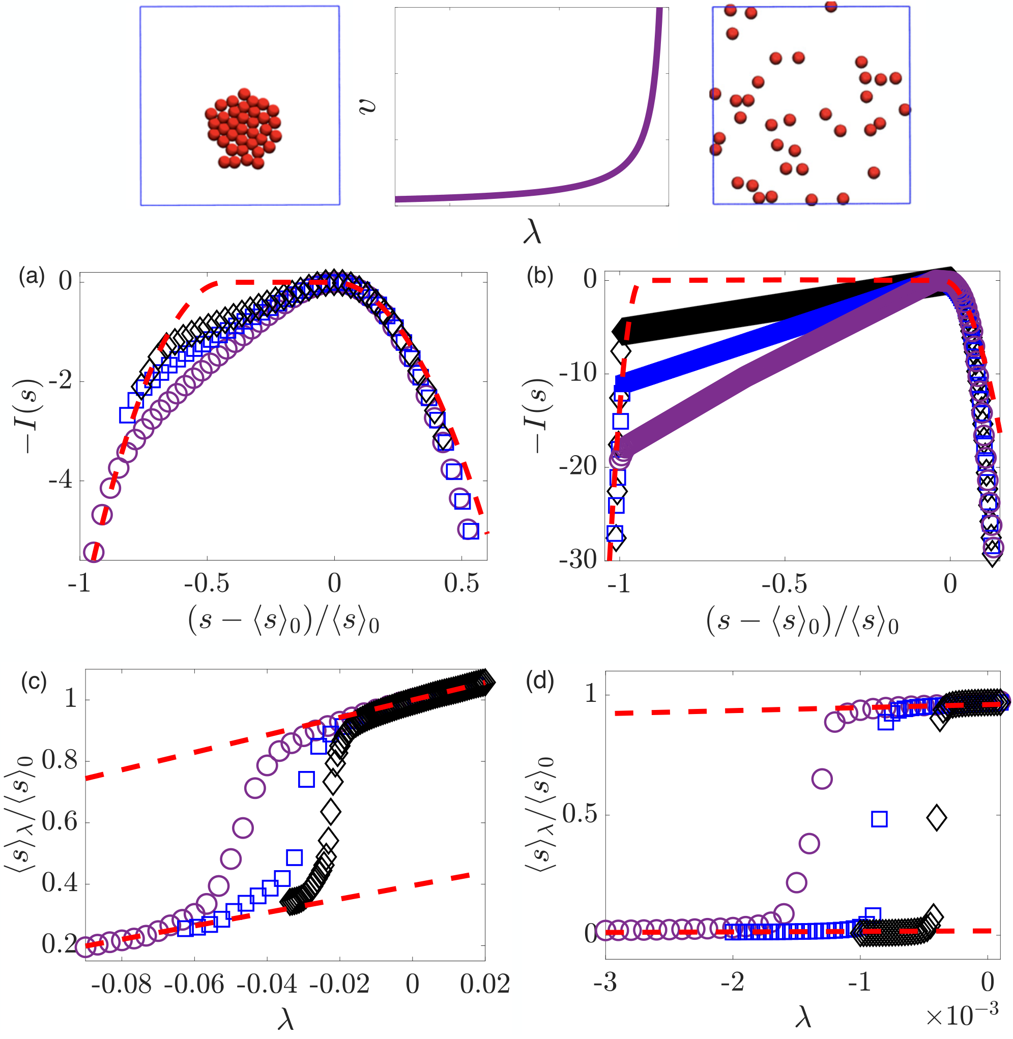
In order to understand the origins of the deviations from the bound and the connections to collective behavior in active matter, we consider in detail a system of ABPs at conditions near and far from its motility induced phase separation (MIPS) transition. Additionally, the asymmetry of entropy production fluctuations about its average, motivates us to consider separately fluctuations of $s>\langle s\rangle_{0}$ and $s<\langle s\rangle_{0}$. In Fig. 2, the distributions for $s>\langle s\rangle_{0}$ are shown for $v=10$ and $v=120$, for a variety of system sizes at fixed density, $\rho=0.1$. While the probability is larger than predicted by the bound, it can be perturbatively corrected. Specifically, we can expand Eq. 5 up to the second cumulant, $\psi(\lambda)\approx\psi_{f}(\lambda)+\left(\lambda\left\langle\Delta W\right\rangle_{0}+\lambda^{2}\left\langle\delta\Delta W^{2}\right\rangle_{0}/2\right)/Nt$. The result of this approximation to the rate function is shown in Figs. 2 a) and b). For $v=10$ the fluctuations are well described by the cumulant approximation, while for $v=120$ asymptotic entropy production fluctuations are narrower than predicted.

The asymptotic behavior for $s\gg\langle s\rangle_{0}$ is well described by free particle motion for all $v$’s. This can be seen by considering $d\psi/d\lambda=\langle s\rangle_{\lambda}$ from $\langle s\rangle_{\lambda}=\int ds\,s\exp\{Nt[-I(s)+\lambda s-\psi(\lambda)]\}$, which is a direct probe of the tails of $I(s)$. As shown in Figs. 2 c) and d), for both large and small $v$, $\langle s\rangle_{\lambda}$ exhibits a crossover from Gaussian statistics. Near $\lambda=0$, $\langle s\rangle_{\lambda}$ varies linearly with $\lambda$ with a slope given by the variance $\langle\delta s^{2}\rangle_{0}$. For $\lambda\gg 0$, $\langle s\rangle_{\lambda}$ varies linearly with $\lambda$ with a slope given by the free particle variance. An analogous crossover has been noted in the current statistics of an interacting tagged ABP GrandPre and Limmer 2018. The asymptotic free behavior implies that the most likely way for the system to produce large amounts of entropy is to suppress density correlations and decrease $\Delta W$. This behavior results from the system adopting a net orientation for the particles’ self-propulsion vector Nemoto et al. 2019; Cagnetta and Mallmin 2020. If the net orientation persists in the thermodynamic limit, it would represent a spontaneous symmetry breaking.

Fluctuations for $s<\langle s\rangle_{0}$ are much larger than predicted by the bound and are collective in origin. Fig. 3 shows the distributions of entropy production and $\langle s\rangle_{\lambda}$ for $v=10$ and $v=120$ at $\rho=0.1$ for 3 system sizes. The distributions in Figs. 3 a) and b) show significant finite size effects for $s<\langle s\rangle_{0}$. In Figs. 3 c), and d), this is evident by a transition between two types of behavior that sharpens with increasing $N$ and occurs at larger $\lambda$ with increasing $v$ over the limited range of system sizes we can study numerically. These features are a hallmark of a dynamical phase transition, in this case between a dilute phase and a phase separated state reminiscent of MIPS Redner et al. 2013; Cates and Tailleur 2015; Chiarantoni et al. 2020. As has been found previously Nemoto et al. 2019, this shows that the most likely way for the system to produce little entropy is to condense, decreasing the particles’ displacement by increasing the effective drag. We find we can describe $I(s)$ by explicitly assuming that each dynamical phase is well approximated by a Gaussian distribution. Specifically, assuming $\psi_{i}(\lambda)Nt=\lambda\langle\Delta S\rangle_{i}+\lambda^{2}\langle\delta\Delta S^{2}\rangle_{i}/2$ for $i={d,c}$ being the dilute and condensed phases, the rate function can be computed from a contraction principle Chetrite and Touchette 2015a for the CGF, $\psi(\lambda)=\max_{\lambda}[\psi_{c}(\lambda),\psi_{d}(\lambda)]$ (see Appendix A). The result is a Maxwell construction and is shown in Fig. 3 to be a good approximation in the infinite system size limit. Due to the exponential difficulty of sampling large deviations in interacting systems we are unable to study larger systems Ray et al. 2018b. Effects from the relatively large persistent length for $v=120$ may complicate the extrapolation of these finite size effects to larger systems.

For $s<\langle s\rangle_{0}$, it is not sufficient to perturbatively correct the bound even for $v=10$, which is far from the MIPS transition. To understand this behavior we have developed a coarse-grained theory. We define a fluctuating density field as $\rho(\bm{r},t)=\sum_{i=1}^{N}\delta[\bm{r}-\bm{r}_{i}(t)]$. With this field, $\Delta W$ can be computed by assuming that the collisions are concentrated directly in front of a tagged particle. Under that assumption, $\Delta W$ can be written in terms of $\rho(\bm{r},t)$, $\Delta W\approx-\beta v\int dt\int d{\bm{r}}d{\bm{r}^{\prime}}\rho(\bm{r},t)F(|\bm{r}-\bm{r}^{\prime}|)\rho(\bm{r}^{\prime},t)/2\,,$ which is a convolution of two points of the density field with the interparticle force. For simplicity we have assumed that $F(0)=0$. Further assuming that the force can be Fourier transformed, we find

where $\hat{\rho}(k,t)$ is the Fourier transformed isotropic density field and $\hat{F}(k)$ the Fourier transformed force.

In order to evaluate the statistics of $\Delta W$, we require an evolution equation for $\hat{\rho}(k,t)$. From the equation of motion for the position and orientation of each particle in the presence of the single particle control force, standard techniques afford an exact equation of motion for $\rho(\bm{r},t)$ Dean 1996. Its solution is complicated by its non-locality and coupling to a polarization field arising from the dynamics of the particle’s orientation (see Appendix E). Rather than deal with it directly, assuming the system is macroscopically homogeneous on the largest scales, we expect the density field to evolve diffusively. Thus, in the limit that $k\rightarrow 0$, the stochastic equation of motion for $\hat{\rho}(k,t)$ takes the form,

where $\mathcal{D}_{\lambda}$ is the effective diffusion constant, $\Delta_{\lambda}$ is the effective mobility, and $\hat{\eta}_{\rho}$ is a complex noise Speck et al. 2015; Tailleur and Cates 2008; Chakraborti et al. 2016; Cates and Tailleur 2015; Dolezal and Jack 2019. Assuming that the polarization field relaxes quickly, and linearizing around a homogeneous density, these parameters can be derived explicitly for each active matter model.

Equation 10 has the form of an independent Ornstein-Uhlenbeck process for each Fourier mode of the density Dolezal and Jack 2019. The CGF for $\Delta W$ can be solved exactly within this approximate linearized dynamics. Defining $\Delta\psi=\psi-\psi_{f}$,

we get an approximate correction to the bound in Eq. (7) due to interparticle correlations. This correction is valid for all positive $\lambda$, but becomes unstable at a critical value $\lambda_{c}\leq 0$ reflecting the breakdown in the linearized evolution equation for $\hat{\rho}(k,t)$. For a finite system with largest wavevector $k=2\pi\sqrt{{\rho}/N}$, the location of the instability is found by setting the discriminant to zero, $\lambda_{c}\approx-4\pi^{2}\mathcal{D}^{2}_{0}{\rho}/\beta v\hat{F}(0)\Delta_{0}N$ where for the short ranged forces considered, we can approximate the force as $\hat{F}(0)$ and we can neglect the $\lambda$ dependence in $v_{\lambda},\mathcal{D}_{\lambda}$, and $\Delta_{\lambda}$. This instability signals the dynamical phase transition that occurs at $\lambda_{c}=0^{-}$ in the thermodynamic limit and whose influence on the dynamics of active matter increases with $v$, and with increasing proximity to MIPS, consistent with the results in Fig. 3. In a phase separated state, $\Delta W$ is a large negative number which counteracts the free particle contribution and reduces the entropy production.

The origin of phase separation can be understood by noting that the optimal control potential which gives rise to rare entropy fluctuations is, for large interparticle separations $r/\sigma\gg 0$ and in the limit $\lambda$ approaches zero (see Appendix E),

The inverse Fourier transform will involve a convolution between the WCA force and $1/k^{2}$ which gives rise to a Bessel Function. Since the WCA potential quickly decays, the long range contribution in real space is a logrithmic potential,

which is attractive for $\lambda<0$ with a magnitude that depends on $v$ and the control force is $\bm{u}_{\lambda}\approx(\beta\lambda v/\mathcal{D}_{0})\nabla\ln r/2$. For negative enough $\lambda$ or large enough $v$, this force will give rise to phase separation. This optimal control force is similar to other passive models near diffusive instabilities Das and Limmer 2019; Tociu et al. 2019; Dolezal and Jack 2019.

The long-ranged effective force demonstrates how effective attractions are introduced by self-propulsion in order to minimize the entropy production. This force is unique and encodes the way in which self-propelled particles interact provided the condition of obtaining a lower than average value of the entropy production. As such, it provides a sharp relationship between entropy production and emergent collective behavior in active matter. Correlations between entropy production and motility induced phase separation have been observed previously at the level of the mean behavior Crosato et al. 2019; Nardini et al. 2017; Nigmatullin and Prokopenko 2019, however this work codifies that relationship on the level of fluctuations.

For both MIPS and the dynamical transition we discuss, phase separation is the result of a diffusive instability where density accumulates due to unbalanced fluxes made possible by the system being kept from thermal equilibrium. We have shown such collective behavior results from the reduction of entropy production and enhancement of density correlations. Large entropy production by contrast, arises through the suppression of density correlations. Thus, our results show how the structure of entropy production fluctuations are intimately connected to long-ranged correlations in active matter. We expect that deviations from the bound derived here can serve as a guide to identify criticality and novel phases of active matter generally.

Acknowledgements We thank Chloe Ya Gao for sharing her cloning code that was adapted for our work, John Bell for discussions and computing resources, and Ahmad Omar for helpful discussions. This research used resources of the National Energy Research Scientific Computing Center (NERSC), a U.S. Department of Energy Office of Science User Facility operated under Contract No. DE-AC02-05CH11231. TGP and DTL were supported by the U.S. Department of Energy, Office of Basic Energy Sciences through Award No. DE-SC0019375. K.K.M was supported by Director, Office of Science, Office of Basic Energy Sciences, of the U.S. Department of Energy under contract No. DEAC02-05CH11231.

References

- Nardini et al. (2017) C. Nardini, É. Fodor, E. Tjhung, F. Van Wijland, J. Tailleur, and M. E. Cates, Physical Review X 7, 021007 (2017).
- Fodor et al. (2020) É. Fodor, T. Nemoto, and S. Vaikuntanathan, New Journal of Physics 22, 013052 (2020).
- del Junco et al. (2018) C. del Junco, L. Tociu, and S. Vaikuntanathan, Proceedings of the National Academy of Sciences 115, 3569 (2018).
- Gaspard and Kapral (2018) P. Gaspard and R. Kapral, The Journal of chemical physics 148, 134104 (2018).
- Dasbiswas et al. (2018) K. Dasbiswas, K. K. Mandadapu, and S. Vaikuntanathan, Proceedings of the National Academy of Sciences 115, E9031 (2018).
- Soni et al. (2019) V. Soni, E. S. Bililign, S. Magkiriadou, S. Sacanna, D. Bartolo, M. J. Shelley, and W. T. Irvine, Nature Physics 15, 1188 (2019).
- Liao et al. (2020) Z. Liao, W. T. Irvine, and S. Vaikuntanathan, Physical Review X 10, 021036 (2020).
- Caballero and Cates (2020) F. Caballero and M. E. Cates, Phys. Rev. Lett. 124, 240604 (2020).
- Fodor et al. (2016) É. Fodor, C. Nardini, M. E. Cates, J. Tailleur, P. Visco, and F. van Wijland, Physical review letters 117, 038103 (2016).
- Mandal et al. (2017) D. Mandal, K. Klymko, and M. R. DeWeese, Physical review letters 119, 258001 (2017).
- Metselaar et al. (2019) L. Metselaar, J. M. Yeomans, and A. Doostmohammadi, Physical Review Letters 123, 208001 (2019).
- Li and ten Wolde (2019) Y. Li and P. R. ten Wolde, Physical review letters 123, 148003 (2019).
- Wang et al. (2019) C. Wang, Y.-k. Guo, W.-d. Tian, and K. Chen, The Journal of chemical physics 150, 044907 (2019).
- Morris and Rao (2019) R. G. Morris and M. Rao, Physical Review E 100, 022413 (2019).
- Bain and Bartolo (2019) N. Bain and D. Bartolo, Science 363, 46 (2019).
- Morin and Bartolo (2018) A. Morin and D. Bartolo, Physical Review X 8, 021037 (2018).
- Bricard et al. (2013) A. Bricard, J.-B. Caussin, N. Desreumaux, O. Dauchot, and D. Bartolo, Nature 503, 95 (2013).
- Mietke et al. (2019) A. Mietke, V. Jemseena, K. V. Kumar, I. F. Sbalzarini, and F. Jülicher, Physical review letters 123, 188101 (2019).
- Morozov (2017) A. Morozov, Science 355, 1262 (2017).
- Souslov et al. (2017) A. Souslov, B. C. Van Zuiden, D. Bartolo, and V. Vitelli, Nature Physics 13, 1091 (2017).
- Ropp et al. (2018) C. Ropp, N. Bachelard, D. Barth, Y. Wang, and X. Zhang, Nature Photonics 12, 739 (2018).
- Takatori and Sahu (2020) S. C. Takatori and A. Sahu, Physical Review Letters 124, 158102 (2020).
- Chaudhuri (2014) D. Chaudhuri, Physical Review E 90, 022131 (2014).
- Pietzonka et al. (2019) P. Pietzonka, E. Fodor, C. Lohrmann, M. E. Cates, and U. Seifert, Phys. Rev. X 9, 041032 (2019).
- Krishnamurthy et al. (2016) S. Krishnamurthy, S. Ghosh, D. Chatterji, R. Ganapathy, and A. Sood, Nature Physics 12, 1134 (2016).
- Zakine et al. (2017) R. Zakine, A. Solon, T. Gingrich, and F. van Wijland, Entropy 19, 193 (2017).
- Martin et al. (2018) D. Martin, C. Nardini, M. E. Cates, and É. Fodor, EPL (Europhysics Letters) 121, 60005 (2018).
- Saha et al. (2018) A. Saha, R. Marathe, P. Pal, and A. Jayannavar, Journal of Statistical Mechanics: Theory and Experiment 2018, 113203 (2018).
- Ekeh et al. (2020) T. Ekeh, M. E. Cates, and E. Fodor, Phys. Rev. E 102, 010101 (2020).
- Chaki and Chakrabarti (2018) S. Chaki and R. Chakrabarti, Physica A: Statistical Mechanics and its Applications 511, 302 (2018).
- Jarzynski (1997) C. Jarzynski, Physical Review Letters 78, 2690 (1997).
- Crooks (1999) G. E. Crooks, Physical Review E 60, 2721 (1999).
- Gallavotti and Cohen (1995) G. Gallavotti and E. G. D. Cohen, Physical review letters 74, 2694 (1995).
- Gaspard and Kapral (2017) P. Gaspard and R. Kapral, The Journal of chemical physics 147, 211101 (2017).
- Horowitz and Gingrich (2019) J. M. Horowitz and T. R. Gingrich, Nature Physics , 1 (2019).
- Di Terlizzi and Baiesi (2018) I. Di Terlizzi and M. Baiesi, Journal of Physics A: Mathematical and Theoretical 52, 02LT03 (2018).
- Owen et al. (2020) J. A. Owen, T. R. Gingrich, and J. M. Horowitz, Physical Review X 10, 011066 (2020).
- Nardini and Touchette (2018) C. Nardini and H. Touchette, The European Physical Journal B 91, 16 (2018).
- Gao and Limmer (2019) C. Y. Gao and D. T. Limmer, The Journal of chemical physics 151, 014101 (2019).
- Dechant and Sasa (2020) A. Dechant and S.-i. Sasa, Proceedings of the National Academy of Sciences 117, 6430 (2020).
- Polettini and Esposito (2019) M. Polettini and M. Esposito, Journal of Statistical Physics 176, 94 (2019).
- Barbier and Gaspard (2018) M. Barbier and P. Gaspard, Journal of Physics A: Mathematical and Theoretical 51, 355001 (2018).
- Epstein and Mandadapu (2020) J. M. Epstein and K. K. Mandadapu, Physical Review E 101, 052614 (2020).
- Hargus et al. (2020) C. Hargus, K. Klymko, J. M. Epstein, and K. K. Mandadapu, The Journal of Chemical Physics 152, 201102 (2020).
- Wagner et al. (2019) C. G. Wagner, M. F. Hagan, and A. Baskaran, Physical Review E 100, 042610 (2019).
- Asheichyk et al. (2019) K. Asheichyk, A. P. Solon, C. M. Rohwer, and M. Krüger, The Journal of chemical physics 150, 144111 (2019).
- Dal Cengio et al. (2019) S. Dal Cengio, D. Levis, and I. Pagonabarraga, Physical Review Letters 123, 238003 (2019).
- Caprini et al. (2018) L. Caprini, U. M. B. Marconi, and A. Vulpiani, Journal of Statistical Mechanics: Theory and Experiment 2018, 033203 (2018).
- Merlitz et al. (2018) H. Merlitz, H. D. Vuijk, J. Brader, A. Sharma, and J.-U. Sommer, The Journal of Chemical Physics 148, 194116 (2018).
- Liao et al. (2019) Z. Liao, M. Han, M. Fruchart, V. Vitelli, and S. Vaikuntanathan, The Journal of chemical physics 151, 194108 (2019).
- Chetrite and Touchette (2015a) R. Chetrite and H. Touchette, in Annales Henri Poincaré, Vol. 16 (Springer, 2015) pp. 2005–2057.
- Barato and Seifert (2015) A. C. Barato and U. Seifert, Physical review letters 114, 158101 (2015).
- Gingrich et al. (2016) T. R. Gingrich, J. M. Horowitz, N. Perunov, and J. L. England, Phys. Rev. Lett. 116, 120601 (2016).
- Lebowitz and Spohn (1999) J. Lebowitz and H. Spohn, Journal of Statistical Physics 95, 333 (1999).
- Seifert (2005) U. Seifert, Physical review letters 95, 040602 (2005).
- Maes and Netočnỳ (2003) C. Maes and K. Netočnỳ, Journal of statistical physics 110, 269 (2003).
- Caprini et al. (2019) L. Caprini, U. M. B. Marconi, A. Puglisi, and A. Vulpiani, Journal of Statistical Mechanics: Theory and Experiment 2019, 053203 (2019).
- Chaki and Chakrabarti (2019) S. Chaki and R. Chakrabarti, Physica A: Statistical Mechanics and its Applications 530, 121574 (2019).
- Cagnetta et al. (2017) F. Cagnetta, F. Corberi, G. Gonnella, and A. Suma, Physical review letters 119, 158002 (2017).
- Nemoto et al. (2019) T. Nemoto, É. Fodor, M. E. Cates, R. L. Jack, and J. Tailleur, Physical Review E 99, 022605 (2019).
- Shankar and Marchetti (2018) S. Shankar and M. C. Marchetti, Physical Review E 98, 020604 (2018).
- Szamel (2019) G. Szamel, Physical Review E 100, 050603 (2019).
- Pietzonka and Seifert (2017) P. Pietzonka and U. Seifert, Journal of Physics A: Mathematical and Theoretical 51, 01LT01 (2017).
- Dabelow et al. (2019) L. Dabelow, S. Bo, and R. Eichhorn, Physical Review X 9, 021009 (2019).
- Speck (2017) T. Speck, arXiv preprint arXiv 1707 (2017).
- Speck (2018) T. Speck, EPL (Europhysics Letters) 123, 20007 (2018).
- Speck et al. (2015) T. Speck, A. M. Menzel, J. Bialké, and H. Löwen, The Journal of chemical physics 142, 224109 (2015).
- GrandPre and Limmer (2018) T. GrandPre and D. T. Limmer, Physical Review E 98, 060601 (2018).
- Giardina et al. (2006) C. Giardina, J. Kurchan, and L. Peliti, Physical review letters 96, 120603 (2006).
- Ray et al. (2018a) U. Ray, G. K.-L. Chan, and D. T. Limmer, Physical review letters 120, 210602 (2018a).
- Weeks et al. (1971) J. D. Weeks, D. Chandler, and H. C. Andersen, The Journal of chemical physics 54, 5237 (1971).
- Cagnetta and Mallmin (2020) F. Cagnetta and E. Mallmin, Physical Review E 101, 022130 (2020).
- Redner et al. (2013) G. S. Redner, M. F. Hagan, and A. Baskaran, Physical review letters 110, 055701 (2013).
- Cates and Tailleur (2015) M. E. Cates and J. Tailleur, Annu. Rev. Condens. Matter Phys. 6, 219 (2015).
- Chiarantoni et al. (2020) P. Chiarantoni, F. Cagnetta, F. Corberi, G. Gonnella, and A. Suma, Journal of Physics A: Mathematical and Theoretical (2020).
- Ray et al. (2018b) U. Ray, G. K.-L. Chan, and D. T. Limmer, The Journal of chemical physics 148, 124120 (2018b).
- Dean (1996) D. S. Dean, Journal of Physics A: Mathematical and General 29, L613 (1996).
- Tailleur and Cates (2008) J. Tailleur and M. Cates, Physical review letters 100, 218103 (2008).
- Chakraborti et al. (2016) S. Chakraborti, S. Mishra, and P. Pradhan, Physical Review E 93, 052606 (2016).
- Dolezal and Jack (2019) J. Dolezal and R. L. Jack, Journal of Statistical Mechanics: Theory and Experiment 2019, 123208 (2019).
- Das and Limmer (2019) A. Das and D. T. Limmer, The Journal of Chemical Physics 151, 244123 (2019).
- Tociu et al. (2019) L. Tociu, É. Fodor, T. Nemoto, and S. Vaikuntanathan, Physical Review X 9, 041026 (2019).
- Crosato et al. (2019) E. Crosato, M. Prokopenko, and R. E. Spinney, Physical Review E 100, 042613 (2019).
- Nigmatullin and Prokopenko (2019) R. Nigmatullin and M. Prokopenko, arXiv:1912.08948 (2019).
- Solon et al. (2015a) A. P. Solon, J. Stenhammar, R. Wittkowski, M. Kardar, Y. Kafri, M. E. Cates, and J. Tailleur, Physical review letters 114, 198301 (2015a).
- Fily et al. (2017) Y. Fily, A. Baskaran, and M. F. Hagan, The European Physical Journal E 40, 1 (2017).
- Löwen (2018) H. Löwen, EPL (Europhysics Letters) 121, 58001 (2018).
- Winkler (2016) R. G. Winkler, Soft matter 12, 3737 (2016).
- Hidalgo et al. (2017) E. G. Hidalgo, T. Nemoto, and V. Lecomte, Physical Review E 95, 062134 (2017).
- Takatori et al. (2014) S. C. Takatori, W. Yan, and J. F. Brady, Physical review letters 113, 028103 (2014).
- Omar et al. (2020) A. K. Omar, Z.-G. Wang, and J. F. Brady, Physical Review E 101, 012604 (2020).
- Touchette (2018) H. Touchette, Physica A: Statistical Mechanics and its Applications 504, 5 (2018).
- Chetrite and Touchette (2015b) R. Chetrite and H. Touchette, Journal of Statistical Mechanics: Theory and Experiment 2015, P12001 (2015b).
- Solon et al. (2015b) A. P. Solon, M. Cates, and J. Tailleur, The European Physical Journal Special Topics 224, 1231 (2015b).
- Bialké et al. (2013) J. Bialké, H. Löwen, and T. Speck, EPL (Europhysics Letters) 103, 30008 (2013).
- Angeletti and Touchette (2016) F. Angeletti and H. Touchette, Journal of Mathematical Physics 57, 023303 (2016).