Silhouette Vectorization by Affine Scale-space
Abstract
Silhouettes or 2D planar shapes are extremely important in human communication, which involves many logos, graphics symbols and fonts in vector form. Many more shapes can be extracted from image by binarization or segmentation, thus in raster form that requires a vectorization. There is a need for disposing of a mathematically well defined and justified shape vectorization process, which in addition provides a minimal set of control points with geometric meaning. In this paper we propose a silhouette vectorization method which extracts the outline of a 2D shape from a raster binary image, and converts it to a combination of cubic Bézier polygons and perfect circles. Starting from the boundary curvature extrema computed at sub-pixel level, we identify a set of control points based on the affine scale-space induced by the outline. These control points capture similarity invariant geometric features of the given silhouette and give precise locations of the shape’s corners.of the given silhouette. Then, piecewise Bézier cubics are computed by least-square fitting combined with an adaptive splitting to guarantee a predefined accuracy. When there are no curvature extrema identified, either the outline is recognized as a circle using the isoperimetric inequality, or a pair of the most distant outline points are chosen to initiate the fitting.
Given their construction, most of our control points are geometrically stable under affine transformations. By comparing with other feature detectors, we show that our method can be used as a reliable feature point detector for silhouettes. Compared to state-of-the-art image vectorization software, our algorithm demonstrates superior reduction on the number of control points, while maintaining high accuracy.
1 Introduction
A silhouette is a subset of the plane that was traditionally obtained by copying on paper the shadow projected on a wall by a person placed in front of a point light source11 1 https://en.wikipedia.org/wiki/Silhouette. In digital images, silhouettes of objects can be obtained by a mere luminance threshold (e.g. Otsu’s algorithm [11]) as soon as the object is darker or brighter than its surroundings. Then the silhouette appears as one of the connected components of an upper or lower set of the image. More generally, the study of shape promoted by Mathematical Morphology [24] calls 2D shapes any such connected component. We will call our object of study here 2D shape or silhouette. Silhouettes are essential for the human perception of shapes, and the distribution of corners along its outlines are closely linked to the neurological models of the visual system [9]. The geometric features captured by the vectorization are important in feature identification [30], remote sensing [21], and others [43, 41, 44]. As proved in [7], if a closed subset of the plane has finite perimeter, then it can be described by its essential boundary, which is a countable set of Jordan curves with finite length. In image processing upper level sets can be extracted by a mere thresholding, in which case they are a finite union of pixels, bounded by a finite number of Jordan curves made of vertical and horizontal segments. Using a parametric interpolation such as the bilinear, one can also extract the boundary of a level set as a union of pieces of hyperbolae [14]. Following [26] an image can therefore be decomposed in a tree of connected shapes ordered by inclusion, and each of these shapes (or silhouettes) can be described by its raster or by its boundary, which is a finite number of Jordan curves described as polygons or concatenations of pieces of hyperbolae.
Thus, there is a standard way to lead back image analysis to the analysis of 2D shapes, and eventually to the analysis of its outline, described by a finite set of nested Jordan curves that also are level lines of the image. This is not the only way to extract shapes from images. Any segmentation algorithm divides an image into connected regions. For example, many software vectorization software22 2 See (e.g.) https://en.wikipedia.org/wiki/Adobe_Illustrator or Vector Magic proceed by a mere color quantization which reduces the image to a piecewise constant image and therefore to a union of disjoint 2D shapes. The boundaries of these shapes can then be encoded in Scalable Vector Graphics (SVG) format33 3 https://fr.wikipedia.org/wiki/Scalable_Vector_Graphics.
A crucial point of such vector representation is that it is scalable, and therefore used for all 2D shapes that, like logos or fonts, require printing at many sizes.
Common silhouette vectorization methods from its outline consist of two steps: identification of control points and approximation of curves connecting the control points. In a founding work, Montanari [27] introduced a polygonal approximation of outlines of rasterized silhouettes. After the discrete boundary is traced, the sub-pixel locations of the polygonal vertices are determined by minimizing a global length energy with an loss to the initial outline. In more recent literature, Bézier curves have become widely adopted to replace polygonal lines [29]. Most developments on silhouette outline vectorization use piecewise Bézier curves, or Bézier polygons [35, 18, 28, 31, 43]. Ramer [35] proposed an iterative splitting scheme for identifying a set of control points on a polygonal line such that the Bézier polygon defined by these vertices approximates . The Hausdorff distance between and is constrained to stay below a predefined threshold, and the number of control points is suboptimal. More recently, Safraz [38] proposed an outline vectorization algorithm that splits the outline at corners which are identified without computing curvatures [17], then new control points are introduced to improve curve fitting. The control points produced by some of these works may correspond to curvature extrema of the outline, but this happens by algorithmic convergence rather than by design. It is well-known that the direct computation of curvature is not reliable [6]. The above mentioned methods reflect the challenges of estimating the outline’s curvature on shapes extracted from raster images.
In this paper, we propose a mathematically founded outline vectorization algorithm. It identifies (i) curvature extrema of the outline computed at sub-pixel level by (ii) backpropagating control points detected as curvature extrema at coarser scale in the affine scale-space, then (iii) computing piecewise least-square cubic Bézier joining these control points while fitting the initial outline with a predefined accuracy.
The main contribution of this paper is to propose a new approach using the sub-pixel curvature extrema and affine scale-space for silhouette vectorization. We shall illustrate by comparisons how the proposed method can give an accurate vectorization with a generally smaller number of more meaningful control points.
We organize the paper as follows. In section 2, an overview of proposed algorithm is presented. In Section 3, we review the level line extraction and sub-pixel curvature computation [19]. In Section 4, we introduce the affine scale-space induced by the smooth bilinear outline and define the candidate control points. In Section 5, we describe an adaptive piecewise least-square Bézier polygon fitting, where the set of candidate points is modified to achieve a compact representation and to guarantee a predefined accuracy. The overall algorithm is summarized in Section 6. We include various numerical results and comparison with other vectorization methods in Section 7, and conclude the paper in Section 8.
2 Overview of the Proposed Method
On a rectangular domain with and , a silhouette is a compact subset whose topological boundary , the outline, is a piecewise smooth curve. Suppose is represented by a raster binary image , that is, the set of black pixels
| (1) |
approximates . We assume that . Our objective is to find a cubic Bézier polygon close to in the Hausdorff distance. The proposed silhouette vectorization method has three main steps:
- 1.
Estimate the curvature extrema of across different scales in sub-pixel level.
- 2.
Based on the affine scale-space induced by , identify salient curvature extrema which are robust against pixelization and noise as the candidate control points.
- 3.
Fit the outline using a Bézier polygon from the candidate control points which are adaptively modified to achieve a compact representation while guaranteeing a desired accuracy.
In the following sections, we give the details of the proposed method.

3 Sub-pixel Curvature Extrema Localization
Following the work of [19], we consider the bilinear interpolation for the raster image whose continuous function form is
| (2) |
where are scalar functions depending on , and
| (3) |
Here is the floor function giving the greatest integer smaller than the real number . For any , the level line of corresponding to is defined as . Since is binary, the Hausdorff distance between any and the raster silhouette (1) is bounded above by . Hence for an arbitrary level approximates the discrete outline as a piecewise Jordan curve except for at finitely many points, e.g., saddle points [15]. In the following, we focus on a single level line for some extracted by the level line extraction algorithm detailed in [16].
Specifically, is either piecewise linear line (horizontal or vertical) or a part of a hyperbola whose asymptotes are adjacent edges of a single pixel. See Figure 1 (c). Due to pixelization, shows strong staircase effects [13], and such oscillatory behavior is effectively reduced by the affine shortening flow [13, 37]. For any planar curve , we smooth it via solving the PDE
| (4) |
to some short time . Here each curve is arc-length parametrized for any , denotes the curvature, and is the inward normal at . The flow (4) is affine intrinsic, that is, its solution is invariant under affine transformations; hence it preserves the geometric properties of the original curve during the evolution.
| (a) | (b) |
|---|---|
 |
 |
To solve (4), we apply the fully consistent geometric scheme [25] which is independent of grid discretization. The idea is that by iterating the discrete affine erosion with a sufficiently small parameter, the convergent morphological operator becomes equivalent to the differential operator in (4). Given a discrete curve partitioned by its inflection points, the -affine erosion of each covex component is a polygonal line whose vertices are the middle points of -chords. See Figure 2. A -chord is a segment joining two points on the curve such that the area enclosed by the segment and the curve is . After the erosion, we glue the evolved components at the inflection points, resample the resulted curve by arc-length, and iterate the procedure above to reach the desired scale . For a sufficiently smooth convex curve, applying the -affine erosion is equivalent to solving (4) till time for some absolute constant [25].
Denoting the smooth bilinear outline obtained above by , the curvature at any of its vertices can be computed without dependence on the grid discretization. The following discussion applies for each connected component. Suppose with and is oriented same as . Following [19], the discrete curvature at point is computed by
| (5) |
where
| (6) |
, and denotes the Euclidean -norm. It computes the discrete curvature of at as the curvature of the circumcircle that passes through three consecutive points , , and . The discrete curvature values can be obtained at arbitrary resolution based on the sampling frequency applied to the bilinear outline , hence it is called “curvature microscope”.
To identify the curvature extrema, we process the data by repeatedly applying the filter with periodic boundary condition for times to suppress the noise. Based on the filtered data , is a curvature extramum if
| (7) |
In practice, to further stabilize the identification, we also require that a curvature extremum should have for some small value . In this paper, we take .
Remark 3.1.
Our method is also applicable when the input is a raster gray-scale image where the intensity variation concentrates around the topological boundary of the underlying silhouette. The higher the image gradient across the silhouette’s boundary, the more stable the position of the extracted outline with respect to the choice of levels.
4 Affine Scale-space Control Points Identification
The curvature extrema form a good set of control points, since they capture the geometrical changes in the outline. We propose to refine the control points via affine scale-space approach, which is detailed in this section.
4.1 Backward Tracing via Inverse Affine Shortening Flow
The concept of scale-space, first introduced by Witkin [42], provides a formalism for multiscale analysis of signals. Later developments [5, 10, 32, 22] established the axiomatic properties for defining a scale-space. In [37], Sapiro et al. proved that the solution of the affine shortening flow (4) defines an affine scale-space, where the scale is given by the time parameter, and the solution at any scale is affine invariant, i.e., it commutes with planar special affine transforms. A critical property satisfied by the affine scale-space is causality: no new information is created when passing from fine to coarse scales. In particular, the following is proved in [37]:
Proposition 4.1.
In the affine invariant scale-space of a planar curve, the number of vertices, that is, the extrema of Euclidean curvature, is a nonincreasing function of time.
More precisely, every curvature extremum on the curve at a coarser scale is the continuation of at least one of the extrema at a finer scale. The lack of one-to-one correspondence is due to the possibility of multiple extrema (e.g. two maxima and one minimum) merging to a single one during the evolution.
In this paper, we propose a new approach for defining the control points as the curvature extrema on which persist across different scales in its affine scale-space. By inversely tracing curvature extrema from the coarser scales to the finer scales, the proposed control points are more robust to noise and help to capture prominent corners of the silhouette.
Given a sequence of discrete times for some positive integer , we obtain the curve at scale by the affine shortening flow (4) for . For any , by a first order Taylor expansion, the affine shortening flow (4) is approximated as
| (8) |
where and denote the curvature and normal at the scale , and is a remainder such that . Rearranging (8) gives
| (9) |
This expression shows that, if is sufficiently small, by following the opposite direction of the affine shortening flow at , that is,
| (10) |
we can find nearby. Here denotes the sign function which gives if , if and if . This gives a well-defined map from the curve at a coarser scale to a finer scale via the inverse affine shortening flow.
Starting from , for any curvature extremum on , we set up the following constrained optimization problem to find a curvature extremum on at scale :
| (11) |
where is a positive parameter that controls the closeness between and , and enforces that the direction of is similar to that of the inverse affine shortening flow. The problem (11) looks for the curvature extremum on in the -neighborhood of that is the nearest to the line passing in the direction of the inverse affine shortening flow. When and are properly chosen, if (11) has one solution, we define it to be . If (11) has multiple solutions, we choose the one that has the shortest distance from to be . In case there are multiple solutions having the same shortest distance from , we can arbitrarily select one to be . However, in practice, if (11) has a solution, it is almost always unique.
We repeat the optimization (11) for , , etc. Either the solutions always exist until the scale , or there exists some , such that (11) at does not have any solution. In the first case, we call a complete point, and in the second case, we call it incomplete. For each curvature extremum on , we construct a sequence of points that contains the solutions of (11) for , etc., starting at in a scale-decreasing order. If is complete, then has exactly elements, and we call the sequence complete; otherwise, the size of is strictly smaller than , and we call the sequence incomplete.
We define the last elements of the complete sequences as the candidate control points, and denote them as . This set of points is ordered following the orientation of . Here the parameter in the parenthesis indicates that the candidate control points are associated with the curvature extrema identified at the scale . When the scale is fixed, we simply write .
4.2 Degenerate Case
In the discussion above, if , i.e., if there are no candidate control points identified on associated with the curvature extrema at scale , then we call it a degenerate case. This situation occurs when the underlying silhouette is a disk, or has a smoothly varying boundary, provided that the image has sufficiently high resolution. This paper is not considering open curves. If we did, the absence of curvature extrema only means that the curve has a monotone curvature, hence is a spiral.
If is indeed a disk, the vectorization only requires information about its center and radius. We use the isoperimetric inequality to determine if represents a circle: for any closed plane curve with area and perimeter , we have
| (12) |
and the equality holds if and only if the curve is a circle. In practice, we decide that is a circle only if the corresponding ratio . By this criterion, if is classified as a circle, then its center and radius are easily computed by arbitrarily three distinct points on . For numerical stability, we take three outline points that are equidistant from each other.
When for a degenerate case, we insert a pair of most distant points on to be the candidate control points. An efficient approach for finding these points is to combine a convex hull algorithm, e.g., the monotone chain method [8], which takes time, with the rotating calipers [34], which takes time. Here is the number of vertices of the polygonal line .
5 Adaptive Cubic Bézier Polygon Approximation
Starting from the control points identified by the affine scale-space, , we adjust by deleting non-salient sub-pixel curvature extrema and inserting new control points for guaranteeing a predefined accuracy. This adaptive approach yields a cubic Bézier polygon whose vertices are points in the updated and edges are cubic Bézier curves computed by least-square fittings.
5.1 Bézier Fitting with Chord-length Parametrization
A cubic Bézier curve is specified by four points , and . Its parametric form is
| (13) |
Specifically, it has the following properties: (i) and are the two endpoints for ; and (ii) is the right tangent of at , and is the left tangent at . To approximate a polygonal line segment , we find a cubic Bézier curve that is determined by , , , and such that the squared fitting error
| (14) |
is minimized. Here is the chord-length parameter for , . We note that (14) is used to initialize an iterative algorithm in [33] for a more accurate Bézier fitting. The benefit of this approximating setup is that we have closed-form formulae for the minimizing and as follows:
| (15) |
where
and
Hence we gain a better computational efficiency. A similar strategy is also taken in [28] to find a Bézier cubic to smooth discrete outlines.
5.2 Control Point Update: Deletion of Sub-pixel Extrema
Recall that the candidate control points in Section 4 are curvature extrema at sub-pixel level. Hence it is possible that some of them do not reflect salient corners of the silhouette. To remove spurious sub-pixel extrema from , we propose to compare the left tangent and right tangent at each candidate control point, which are obtained via the least-square cubic Bézier fitting discussed above.
We take advantage of the second property of cubic Bézier curves mentioned in Section 5.1. For , we fit a cubic Bézier to the polygonal line segment whose set of vertices is
| (16) |
where we take , and obtain the estimated defining points and for the Bézier curve. The left and right tangent at are computed as
| (17) |
respectively, where . These tangent vectors are associated with all the points between neighboring candidate control points. Therefore, the angle formed by and measures the sharpness of at from a more global perspective. We delete from the set of candidate control points if
| (18) |
for some small parameter , which is equivalent to the condition that the angle between and is close to . The set is updated with the remaining control points.
It is possible that all the candidate control points are removed after this procedure, thus we encounter a degenerate case. If the underlying outline is a circle, we compute the center and radius; if it is not, we take the most distant pair of outline points to update .
5.3 Control Point Update: Insertion for Accuracy
The candidate control points in split the outline into polygonal line segments, each of which is approximated by a cubic Bézier using least square fitting as described in Section 5.1. We obtain a Bézier polygon that approximates , denoted by . A natural measure for the error of approximating using the Bézier polygon is
| (19) |
where is the distance from to the curve . It is desirable that the user can specify the threshold for the error, . To guarantee that , we apply the splitting strategy [35] which inserts to as a new control point if
| (20) |
and among those points on satisfying (20), is the largest. After the insertion, we fit using a Bézier polygon based on the new set of control points in . If the error of the newly fitted Bézier polygon is still greater than , we insert another point based on the same criterion. This series of insertions terminates once the condition is met.
Finally, with the updated set of control points gives a Bézier polygon that approximates the outline , and with its interior filled with black, we obtain the vectorized silhouette for from the raster image .
Remark 5.1.
For a further reduction on the size of , we may consider an optional step to merge neighboring Bézier cubics if the union of the underlying polygonal line segments can be approximated by a single Bézier cubic via (14) with an error below . We can regard the insertion in Section 5.3 as controlling the data fidelity, and the simplification described here as minimizing the complexity of an estimator. Alternatively iterating these procedures provides a numerical scheme for a constrained optimizing problem
where denotes the number of elements in . For any , this problem always has a solution, yet the uniqueness largely depends on the geometric structure of .
6 Pseudo-code for the Proposed Method
In this section, assuming that the outline of the given silhouette has only one connected component, we summarize the proposed algorithm for silhouette vectorization in three steps:
- 1.
Extraction of the smooth sub-pixel outline Extract the level line corresponding to from the bilinear interpolation of the image, then discretize it as a polygon with uniform sub-pixel sampling. To reduce the staircase effects, smooth the polygon via affine shortening at a scale specified by the smoothness parameter . In this paper, we take .
- 2.
Identification of candidate control points. Fix an increment and a positive integer . Evolve via the affine shortening using the scales , . Starting from each curvature extremum at scale , trace the curvature extrema at smaller scales along the inverse affine shortening flow as described by (11). By doing so, each curvature extremum at scale induces a sequence of traced curvature extrema across different scales, which are arranged in a scale-decreasing order. The final elements of the complete sequences are defined as the candidate control points, denoted by . In this paper, we fix and , so that .
In case , process the degenerate case as described in Section 4.2.
- 3.
Refinement of the control points. Remove any candidate control point from whose left tangent and right tangent (17) form an angle close to (20). If all the candidate control points are removed, follow the instruction in Section 4.2 to address the degenerate case. Then, insert new control points into by the splitting strategy [35] until the approximation error (19) is bounded by a user-specified threshold .
- 4.
(Optional) Merging neighboring Bézier cubics For , delete from if the polygonal line segment bounded by the left and right neighboring control points of in can be fitted by a single Bézier cubic with error smaller than .
As for the output, if is not a circle, we write the points in together with the estimated defining points (15) for each segment into a SVG format with the specification of drawing cubic Bézier curves. For the visualization purpose, if a fitted Bézier curve has a maximal absolute curvature smaller than , we assign a straight line. Note that this value is consistent with the value for in Section 3. If is a circle, we write its estimated center and radius into the SVG with the specification of drawing a circle. The pseudo-codes are presented in Algorithm 1 (with sub-procedures described in Algorithm 2 and Algorithm 3), which can be parallelized to apply to outlines with multiple connected components.
7 Numerical Results
In this section, we present some numerical experiments to demonstrate the performance of our proposed algorithm. After obtaining the SVGs from [3], we rasterize them as PNG images, which are used as inputs in the following experiments. The inputs are either binary or gray-scale. We choose the level line corresponding to to approximate the outlines throughout the experiments. By default, we set the error threshold , so that the vectorized outline is guaranteed to have sub-pixel level of accuracy; and the smoothness parameter . For the parameters in (11), we fix and . The silhouettes used in the following experiments are collectively displayed in Table 3. If without any specifications, we apply the proposed method without the optional merging step.
General Performance
We present some results of the our proposed algorithm in Figure 3. In (a), we have a silhouette of a cat. It has a single outline curve which contains multiple sharp corners on the tail, near the neck and around the paws, etc. These features provide informative visual cues for silhouette recognition, and our algorithm identifies them as control points for the silhouette vectorization shown as the red dots in (b). The outline of a butterfly in (c) has multiple connected components. In addition to the control points corresponding to corners, we observe in (d) some others on smooth segments of the outline. They are inserted during the refinement step of our algorithm, where a single Bézier cubic is inadequate to guarantee the accuracy specified by the error threshold . In (e), we show a tessellation of words and (f) presents the vectorized result. The input is a PNG image of dimension and takes KB in the storage. In contrast, its silhouette vectorization, saved as a SVG file, has in total control points and takes KB if the coordinates are stored in float, Kb if stored in integers. In this example, our algorithm provides a compresion ratio of about for float type, and a compression ratio for the integer type. Moreover, the total computational time for this case only takes seconds. Similar statistics for the other two examples are summarized in Table 1. Our algorithm is both effective and efficient.
| (a) | (b) |
 |
 |
| (c) | (d) |
 |
 |
| (e) | (f) |
 |
 |
| (g) | (h) |
 |
 |
| Shape | Image Dim. | Size | Result Size (float) | Result Size (int) | Proc. Time |
|---|---|---|---|---|---|
| Cat (a) | KB | KB () | KB () | Sec. | |
| Butterfly (c) | KB | KB () | KB () | Sec. | |
| Text (e) | KB | KB () | KB () | Sec. |
Degenerate Cases
An important feature of our algorithm is that it offers flexibility in face of degenerate cases, where the silhouette does not have identifiable curvature extrema on its outline. A disk, as shown in Figure 4 (a), is the most common example. Once our algorithm classifies the outline as a circle, instead of fitting Bézier cubics, it directly approximates the center and radius of the circle and orders the SVG output to draw a perfect circle. See Figure 4 (b).
Figure 4 (c) shows another degenerate case. It consists of a rectangle in the middle and two half disks attached on its opposite sides, whose diameters are equal to the height of the rectangle. This particular silhouette has no strict curvature extrema on its outline. By computation, its area is and perimeter is ; since , the outline is not a circle. Hence the algorithm inserts a pair of most distant points on the outline, the left-most and the right-most points in this case, and conducts the Bézier fitting routine as in the non-degenerate cases.
The design of this special procedure for degenerate cases is important for two reasons. First, it makes the algorithm adaptive to image resolutions. If we reduce the resolution of (c) from to , whose magnified version is shown in (e), due to strong effects of pixellization, all the control points are identified as local curvature extrema. (f) shows the magnified vectorization of the low resolution image. Second, it improves the compression ratio. To fit a circle using Bézier polygon requires at least two pieces of cubics, hence we need to store the coordinates of at least points. With our algorithm, only the coordinate of the center and the value of the radius are required, which saves the space for float or int type data. Figure 4 (g) shows mixture of degenerate and non-degenerate outline curves. The vectorization in (h) shows that the circles are represented as perfect circles, and the others are represented as Bézier polygons.
| (a) | (b) |
 |
 |
| (c) | (d) |
 |
 |
| (e) | (f) |
 |
 |
| (g) | (h) |
 |
 |
Importance of the Control Point Update
Figure 5 compares the vectorization using control points before and after the control point update, which are described in Section 5.2 and 5.3. The outline of the knot silhouette in (a) shows curvature variations of multiple scales. If no refinement is applied, as shown in (b), the corners of larger scale are captured, while some inflection points are missed on the top-left component. Moreover, many unnecessary control points appear on several arcs. In contrast, with the refinement, the result in (c) has fewer control points, but with a better approximation accuracy. Notice that on the top-left component of the knot, the newly inserted control points are close to the inflection points, and on the arcs, only or control points are generally needed.
By refinement, we remove extrema that do not represent salient corners and inset new control points to meet the accuracy requirement. Although the total number of control points may or may not decrease after refinement, the distribution of the refined control points shows more correlation with the geometric features of the outline, and the vectorized result is improved.
| (a) | (b) | (c) |
|---|---|---|
 |
 |
 |
Effect of the Error Threshold
The error threshold controls the accuracy of the Bézier polygon approximating the outline. When the value of is reduced, the user requires higher accuracy of the Bézier fitting. Since any Bézier cubic contains at most one inflection point, a single cubic only allows a limited amount of variations. Hence, by adding more control points to split the outline into shorter segments, the specified accuracy is achieved.
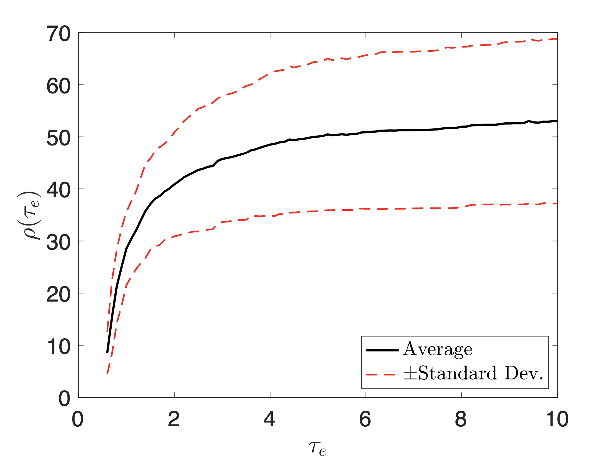
To better illustrate the effect of varying the threshold , we computed in percentage the reduction of the number of control points when the threshold is compared to that when the threshold is :
| (21) |
Here denotes the number of control points when the threshold is . Figure 6 (a) shows the average values and the standard deviations of (21) when we apply the proposed method to the silhouettes in our data set. We observe that when , the effect of increasing is the strongest: the number of control points reduces exponentially. On average, the percentage curves show inflection points around , that is, when the fitted Bézier polygon has distance to the sub-pixel outline less than 1 pixel. After passing , increasing has less impact on the variation of the number of control points. For even larger values of , there is almost no need of inserting new control points, and the corresponding control points are closely related to the corners of the outline. This is justified by the regression in Figure 6 (b), where each point represents a silhouette in our data set. It shows that there is a positive relation between the number of corners computed by the Harris-Stephens corner detector [20] and the number of control points when , which is relatively large.
With large values of , the silhouette representation is more compact yet less accurate. With small values of , we have a more accurate representation yet less efficient. From this point of view, we would recommend .
| (a) | (b) |
|---|---|
 |
 |
Effect of the Smoothness Parameter
The smoothness parameter adjusts the regularity of the smooth bilinear outline which approximates . With larger values of , oscillatory features of the given outline are suppressed, while with smaller values of , the vectorized silhouette preserves sharp corners.
Figure 7 demonstrates this effect of . We apply the proposed method using , and on the silhouette of a tree (a), and the zoom-ins of vectorization results within the boxed region of (a) are presented in (b), (c), and (d), respectively. Observe that the zig-zag feature around the tree’s silhouette is better preserved by reducing . As a trade-off, this introduces more control points to recover the sharpness of the outline.
| (a) | (b) | (c) | (d) |
|---|---|---|---|
 |
Stability Under Affine Transformations
We qualitatively explore the geometric stability of the proposed control points under affine transformations. Figure 8 (a) shows a silhouette of a cat. (b) is a rotation of (a), and (c) is a sheared (a). The vectorized results of these silhouettes are presented in (d), (e), and (f), respectively. To better compare the distributions of the control points on these vectorized outlines, we applied the corresponding inverse affine transformations to (d)–(f) and show the results in (g)–(i). The numbers of control points are similar: (g) has control points ( before refinement), (h) has control points ( before refinement), and (i) has control points ( before refinement). The distributions of control points between (g) and (h) are almost identical, while locations of the control points in (i) are slightly shifted, especially those on the tail. This is because Bézier fitting is not affine invariant, and these shifted points are inserted to guarantee the accuracy of approximating the transformed outline using a Bézier polygon.
| (a) | (b) | (c) |
 |
 |
 |
| (d) | (e) | (f) |
 |
 |
 |
| (g) | (h) | (i) |
 |
 |
 |
Qualitative Comparison with Feature Point Detectors
Our algorithm produces a set of informative point features of the outline. This includes the control points which separate the outline curves into segments for cubic Bézier fitting and the centers of circles. In Figure 9, we compare the distribution of these points with the results of some extensively applied feature point detectors: the Harris-Stephens corner detector [20], the features from Accelerated Segment Test (FAST) detector [36], the Speeded Up Robust Features (SURF) detector [12], and the Scale-Invariant Feature Transform (SIFT) [23].
The Harris-Stephens corner detector is a local auto-correlation based method. It locally filters the image with spatial difference operators and identifies corners based on the response. In (a), the Harris-Stephens corner detector identifies all the corners except for the one on the right side of the label. The set of control points produced by our algorithm contains all the corners found by the Harris-Stephens detector plus the missed one.
The FAST detector only considers the local configurations of pixel intensities, hence it is widely applied in real-time applications. From (b), we see that FAST identifies all the prominent corners same as our method does. Similarly to (a), there are no FAST points identified around the balloon. On the circular outline at the center instead, FAST detects multiple false corners; this illustrates how our algorithm is more robust against pixellization
The SURF detector combines a fast Hessian measure computed via integral images and the distribution of local Haar-wavelet responses to identify feature points that are scale- and rotation-invariant. There is a similarity that it utilizes the Gaussian scale-space and scale-space interpolation to localize the points of interest. The SURF points are marked over scales, hence we see most of the green crosses in (c) form sequences converging toward the outline. These limit points correspond exactly to our control points (red dots) distributed over the outline, including those around the balloon. Moreover, there is a SURF point at the center of the circular hole in the label, which overlaps with our identified center of circle (blue dot). Rather than showing feature points over scales, our method locates them directly on the original outline. In (c), notice that our identified points are much simpler compared to SURF points.
The SIFT detects scale-invariant features of a given image. As shown in (d), SIFT successfully indicates the presence of corners and marks the centers of the balloon as well as the label, which are visually robust features of the silhouette Our method focuses on the outline instead of the interior points and provides interesting boundary points’ locations exactly. Around the balloon, the symmetric distribution is compatible with the SIFT point at the center.
The set of control points plus the center of circles produced by our algorithm is comparable to some of the frequently used feature point detectors in the literature. Hence,in addition to being an effective silhouette vectorization method, the identified control points can be used for other applications where feature point detectors are needed.
| (a) | (b) | (c) | (d) |
|---|---|---|---|
 |
 |
 |
 |
Quantitative Comparison with Feature Point Detectors
To further justify that our method can be applied as a stable point feature detector for silhouettes, we compare the techniques discussed above with ours by quantitatively evaluating their performances via the repeatability ratio [39]. It measures the geometric stability of the detected feature points under various transformation.
In particular, for each method, given any angle , , we rotate the silhouettes in the first column of Figure 10 with respect to their centers by respectively, record the detected feature points, apply the inverse transform on these points by rotating them by , then compare their positions with the feature points detected on the original silhouette. Let . For any rotated feature point, within its -neighborhood, if we find at least one feature point on the original silhouette, we increase by . The -repeatability ratio is computed by
| (22) |
where denotes the number of feature points detected on the original silhouette, and is the number of feature points detected on the transformed one. During the angle (or scale) changes, this value staying near indicates that the applied method is invariant under rotation (or scale). We fix .
The second column of Figure 10 shows the repeatability ratios under rotations. The set of feature points produced by our method has superior stability when the silhouette is rotated by arbitrary angles. In contrast, the other detectors have low repeatability ratios especially when the silhouette is turned almost upside-down. Moreover, our method performs consistently well for silhouettes with different geometric features. The house silhouette has straight outlines and sharp corners; the butterfly silhouette is defined by smooth curves; and the fish silhouette has prominent curvature extrema which are not perfect corners.
For the third column of Figure 10, we compute the repeatability ratios when the transformation is replaced by scaling. Observe that our method is comparable with other detectors, and it is the most consistent one across these different silhouettes.
| Silhouette | Under Rotation | Under Scaling |
|---|---|---|
 |
 |
 |
 |
 |
 |
 |
 |
 |
Comparison with State-of-the-art Software
There are many software available for image vectorization, e.g., Vector Magic [4], Inkspace [2], and Adobe Illustrator 2020 (AI) [1]. In the following set of experiments, we compare our method with these software using the number of control points generated for given silhouettes as a criteria. This quantity is equal to the number of curve segments used for approximating the outline, and a smaller value indicates a more compact silhouette representation.
To perform this comparison, after acquiring SVG files of various silhouettes, we rasterized them and used the PNG images as inputs. Table 2 summarizes the results. For Vector Magic, we test three available settings: high, medium, and low for the vectorization quality. For AI, we choose the setting“Black and White Logo”, as it is suitable for the style of our inputs. We also include the results when the automatic simplification is used, which are marked by daggers. For Inkspace, we use the default parameter settings as recommended. As shown by the values of the mean relative reduction on the number of control points in the last row, our method produces the most compact vectorization results.
With such an effective reduction on the number of control points, we justify that our method does not over-simplify the representation. We show a detailed comparison in Figure 11 between our proposed method and AI. In particular, we use AI without simplification and our method with two sets of parameters: , and , . We note that specifies the smoothness of the recovered outline, and controls the accuracy. Notice that under these settings, our method gives less number of control points, yet our results preserve more details of the given silhouettes, for example, the strokes on the scales at the bottom, and the sharp outlines on the rear fin.
We quantify the performance of AI and our method by comparing the given image and the image rasterized from the vectorization result. Denote and as the interior pixels of the given silhouette and the reconstructed one. We evaluate the similarity between and by
| (23) |
Higher values of DSC imply a better matching between two silhouettes. We evaluate the performance with wide ranges of parameters for both AI and the proposed method. For AI, we test various combinations of the curve simplification parameter (–) and the corner point angle threshold (–). For our method, we use different combinations of and . Roughly speaking, in AI corresponds to in ours, which controls the approximating accuracy, and in AI corresponds to in ours, which adjusts the smoothness of the vectorized outline. Figure 12 plots the number of control points against the corresponding DSC values for various parameter settings in both methods. In (a), we fix the sharpness requirement, i.e., fixed (default value for the automatic simplification used in AI) and fixed , and vary for AI (the blue curve) and for ours (the red curve). On the blue curve, larger dots correspond to smaller values of ; on the red curve, larger dots correspond to larger values of . Moving from left to right along both curves indicates more accurate outline approximations. Since the red curve stays below the blue one, compared to AI, our method produces less control points while achieving the same level of DSC values. In (b), we present the results of AI using simplification specified by a set of combinations of parameters (, ). They are organized such that each blue curve corresponds to a fixed value of ; higher curves (lighter shades of blue) correspond to larger values of , while moving from left to right (smaller sizes of dots) along each of the curves corresponds to decreasing . The red curve shows our results using different values of when the merging is applied and is fixed at . From left to right, the value of decreases. Observe that the red curve gives a close lower bound for the blue curves when DSC. For higher requirement on the accuracy (DSC), our method shows superior efficiency: it takes comparatively small number of control points to reach greater values of DSC. In contrast, for AI, the best DSC value it can achieve is around , and adding more control points does not offer any improvement.
| Number of Control Points () | |||||
| Test Image | Original | VM | IS | AI | Proposed |
![[Uncaptioned image]](2007.12117v1/Figures/panel.png) |
|||||
![[Uncaptioned image]](2007.12117v1/Figures/dog.png) |
|||||
![[Uncaptioned image]](2007.12117v1/Figures/heart.png) |
|||||
![[Uncaptioned image]](2007.12117v1/Figures/map.png) |
|||||
![[Uncaptioned image]](2007.12117v1/Figures/circle.png) |
|||||
![[Uncaptioned image]](2007.12117v1/Figures/fish.png) |
|||||
| MRR | — | ||||

| (a) | (b) |
|---|---|
 |
 |
8 Conclusion
In this paper, we proposed an efficient and effective algorithm for silhouette vectorization. The outline of the silhouette is interpolated bilinearly and uniformly sampled at sub-pixel level. To reduce the oscillation due to pixelization, we applied the affine shortening to the bilinear outline. By tracing the curvature extrema across different scales along the well-defined inverse affine shortening flow, we identified a set of candidate control points. This set is then refined by deleting sub-pixel extrema that do not reflect salient corners, and inserting new points to guarantee any user-specified accuracy. We also designed special procedures to address the degenerate cases, such as disks, so that our algorithm adapts to arbitrary resolutions and offers better compression of information. Our method provides a superior compression ratio by vectorizing the outlines. When the given silhouette undergoes affine transformations, the distribution of control points generated by our method remains relatively stable. These properties are quantitatively justified by the repeatability ratio when compared with popular feature point detectors. Our method is competitive compared to some well-established image vectorization software in terms of producing results that have less number of control points while achieving high accuracy.
Appendix A Silhouette Data Set
In Table 3, we collectively display the silhouettes used in this paper. They are all downloadable from https://svgsilh.com, which are released under Creative Commons CC0.
![[Uncaptioned image]](2007.12117v1/Figures/tree_o.png)
![[Uncaptioned image]](2007.12117v1/Figures/balloon.png)
![[Uncaptioned image]](2007.12117v1/Figures/ant.png)
![[Uncaptioned image]](2007.12117v1/Figures/trophy.png)
![[Uncaptioned image]](2007.12117v1/Figures/note.png)
![[Uncaptioned image]](2007.12117v1/Figures/figure.png)
References
- [1] Adobe Illustrator. https://www.adobe.com/products/illustrator.html.
- [2] Inkspace. https://inkscape.org.
- [3] SVG SILH. https://svgsilh.com. All contents are released under Creative Commons CC0.
- [4] Vector Magic. https://vectormagic.com.
- [5] L. Álvarez, F. Guichard, P.-L. Lions, and J.-M. Morel. Axiomes et équations fondamentales du traitement d’images.(analyse multiéchelle et edp). Comptes rendus de l’Académie des sciences. Série 1, Mathématique, 315(2):135–138, 1992.
- [6] L. Alvarez and J. M. Morel. Formalization and computational aspects of image analysis. Acta numerica, 3:1–59, 1994.
- [7] L. Ambrosio, V. Caselles, S. Masnou, and J.-M. Morel. Connected components of sets of finite perimeter and applications to image processing. Journal of the European Mathematical Society, 3(1):39–92, 2001.
- [8] A. Andrew. Another efficient algorithm for convex hulls in two dimensions. Information Processing Letters, 9(5):216–219, 1979.
- [9] F. Attneave. Some informational aspects of visual perception. Psychological review, 61(3):183, 1954.
- [10] J. Babaud, A. P. Witkin, M. Baudin, and R. O. Duda. Uniqueness of the Gaussian kernel for scale-space filtering. IEEE transactions on pattern analysis and machine intelligence, (1):26–33, 1986.
- [11] J. P. Balarini and S. Nesmachnow. A C++ Implementation of Otsu’s Image Segmentation Method. Image Processing On Line, 6:155–164, 2016.
- [12] H. Bay, T. Tuytelaars, and L. Van Gool. Surf: Speeded up robust features. In European conference on computer vision, pages 404–417. Springer, 2006.
- [13] F. Cao. Geometric curve evolution and image processing. Springer Science & Business Media, 2003.
- [14] F. Cao, J.-L. Lisani, J.-M. Morel, P. Musé, and F. Sur. A theory of shape identification. Springer Science & Business Media, 2008.
- [15] V. Caselles and P. Monasse. Geometric description of images as topographic maps. Springer, 2009.
- [16] V. Caselles and P. Monasse. Geometric Description if Images as Topographic Maps. Springer, 2010.
- [17] D. Chetverikov. A simple and efficient algorithm for detection of high curvature points in planar curves. In International Conference on Computer Analysis of Images and Patterns, pages 746–753. Springer, 2003.
- [18] L. Cinque, S. Levialdi, and A. Malizia. Shape description using cubic polynomial bezier curves. Pattern Recognition Letters, 19(9):821–828, 1998.
- [19] A. Ciomaga, P. Monasse, and J.-M. Morel. The image curvature microscope: Accurate curvature computation at subpixel resolution. Image Processing On Line, 7:197–217, 2017.
- [20] C. G. Harris, M. Stephens, et al. A combined corner and edge detector. In Alvey vision conference, volume 15, pages 10–5244. Citeseer, 1988.
- [21] A. Kirsanov, A. Vavilin, and K. Jo. Contour-based algorithm for vectorization of satellite images. In International Forum on Strategic Technology 2010, pages 241–245. IEEE, 2010.
- [22] J. J. Koenderink. The structure of images. Biological cybernetics, 50(5):363–370, 1984.
- [23] D. G. Lowe. Object recognition from local scale-invariant features. In Proceedings of the seventh IEEE international conference on computer vision, volume 2, pages 1150–1157. Ieee, 1999.
- [24] G. Matheron. Random sets and integral geometry [by] G. Matheron. Wiley New York, 1974.
- [25] L. Moisan. Affine plane curve evolution: A fully consistent scheme. IEEE Transactions on Image Processing, 7(3):411–420, 1998.
- [26] P. Monasse and F. Guichard. Scale-space from a level lines tree. Journal of Visual Communication and Image Representation, 11(2):224–236, 2000.
- [27] U. Montanari. A note on minimal length polygonal approximation to a digitized contour. Communications of the ACM, 13(1):41–47, 1970.
- [28] A. S. Montero and J. Lang. Skeleton pruning by contour approximation and the integer medial axis transform. Computers & Graphics, 36(5):477–487, 2012.
- [29] M. E. Mortenson. Mathematics for computer graphics applications. Industrial Press Inc., 1999.
- [30] C. Nadal, R. Legault, and C. Y. Suen. Complementary algorithms for the recognition of totally unconstrained handwritten numerals. In [1990] Proceedings. 10th International Conference on Pattern Recognition, volume 1, pages 443–449. IEEE, 1990.
- [31] S. Pal, P. Ganguly, and P. Biswas. Cubic bézier approximation of a digitized curve. Pattern recognition, 40(10):2730–2741, 2007.
- [32] P. Perona and J. Malik. Scale-space and edge detection using anisotropic diffusion. IEEE Transactions on pattern analysis and machine intelligence, 12(7):629–639, 1990.
- [33] M. Plass and M. Stone. Curve-fitting with piecewise parametric cubics. In Proceedings of the 10th annual conference on Computer graphics and interactive techniques, pages 229–239, 1983.
- [34] F. P. Preparata and M. I. Shamos. Computational geometry: an introduction. Springer Science & Business Media, 2012.
- [35] U. Ramer. An iterative procedure for the polygonal approximation of plane curves. Computer graphics and image processing, 1(3):244–256, 1972.
- [36] E. Rosten and T. Drummond. Fusing points and lines for high performance tracking. In Tenth IEEE International Conference on Computer Vision (ICCV’05) Volume 1, volume 2, pages 1508–1515. Ieee, 2005.
- [37] G. Sapiro and A. Tannenbaum. Affine invariant scale-space. International journal of computer vision, 11(1):25–44, 1993.
- [38] M. Sarfraz. Vectorizing outlines of generic shapes by cubic spline using simulated annealing. International Journal of Computer Mathematics, 87(8):1736–1751, 2010.
- [39] C. Schmid, R. Mohr, and C. Bauckhage. Evaluation of interest point detectors. International Journal of computer vision, 37(2):151–172, 2000.
- [40] T. A. Sorensen. A method of establishing groups of equal amplitude in plant sociology based on similarity of species content and its application to analyses of the vegetation on danish commons. Biol. Skar., 5:1–34, 1948.
- [41] K. Tombre and S. Tabbone. Vectorization in graphics recognition: to thin or not to thin. In Proceedings 15th International Conference on Pattern Recognition. ICPR-2000, volume 2, pages 91–96. IEEE, 2000.
- [42] A. P. Witkin. Scale-space filtering. In Readings in Computer Vision, pages 329–332. Elsevier, 1987.
- [43] H.-M. Yang, J.-J. Lu, and H.-J. Lee. A bezier curve-based approach to shape description for chinese calligraphy characters. In Proceedings of Sixth International Conference on Document Analysis and Recognition, pages 276–280. IEEE, 2001.
- [44] J. J. Zou and H. Yan. Cartoon image vectorization based on shape subdivision. In Proceedings. Computer Graphics International 2001, pages 225–231. IEEE, 2001.