Gravitational interaction through a feedback mechanism
Abstract
We study the models of Kafri, Taylor and Milburn (KTM) and Tilloy and Diósi (TD), both of which implement gravity between quantum systems through a continuous measurement and feedback mechanism. The first model is for two particles, moving in one dimension, where the Newtonian potential is linearized. The second is applicable to any quantum system, within the context of Newtonian gravity. We address the issue of how to generalize the KTM model for an arbitrary finite number of particles. We find that the most straightforward generalisations are either inconsistent or are ruled out by experimental evidence. We also show that the TD model does not reduce to the KTM model under the approximations which define the latter model. We then argue that under the simplest conditions, the TD model is the only viable implementation of a full-Newtonian interaction through a continuous measurement and feedback mechanism.
I Introduction
Gravity is very well described by General Relativity in terms of space-time deformations caused by mass and energy Tosto 2012. All experiments so far have confirmed the theory, up to the direct detection of gravitational waves by the LIGO collaboration Abbott et al. 2016, although the open problems in Cosmology with dark energy Peebles and Ratra 2003 and dark matter Barack et al. 2019 might eventually call for a different description of gravity.
For decades the scientific community has worked towards formulating a quantum theory of gravity, and many important results have been achieved, yet at present a conclusive answer has not been reached Kiefer 2007; Hossenfelder 2011. The lack of a fully consistent quantum theory of gravity has opened the possibility that gravity might not be fundamentally quantum. The scientific community considered several times the option that gravity might be ultimately classical, and this originated a dispute whether this assumption is compatible with the quantum nature of matter or not Feynman 1995; Diósi et al.; Carlip 2001; Huggett and Callender 2001; Peres and Terno 2001; Wüthrich 2005; Rothman and Boughn 2006; Carlip 2008; Dyson 2013; Ahmadzadegan et al. 2016; Bassi et al. 2017; Tilloy 2018a; Carney et al. 2019; Kumar and Plenio 2020; Donadi et al. 2020, until quite recently, when fully consistent models of Newtonian gravity have been formulated, where matter is quantum and gravity is classical Diósi 1989; Penrose 1996; Diósi 2011; Bowen and Milburn 2016; Khosla and Altamirano 2017; Altamirano et al. 2017a; Khosla and Nimmrichter 2018; Altamirano et al. 2018; Tilloy 2018b; Tilloy 2019. Two of such models were proposed by Kafri, Taylor and Milburn (KTM) Kafri et al. 2014, and by Tilloy and Diósi (TD) Tilloy and Diósi 2017.
In this work we study these two models, which implement Newtonian gravity through a continuous measurement and feedback mechanism, whose detailed description is provided below. The first model refers to two particles moving only in one direction, and the Newtonian potential is linearized. The second model applies to any non-relativistic quantum system, and the full Newtonian interaction is considered.
We address the issue of how to generalize the KTM model for a system of particles (with ), taking into account previous results in the literature Altamirano et al. 2018; Kafri et al. 2015. We find that the most straightforward generalisations are either inconsistent or are ruled out by experimental evidence.
For the TD model, we analyse the requirements for regularizing the dynamics and we explicitly derive its conditions. In particular, we construct a family of smearing functions for the case of local operations and classical communication (LOCC) dynamics, which is described below. Then, in the appropriate limit, we compare the TD and the KTM models, finding that they predict quantitatively different decoherence effects, and thus concluding that the TD model is not a generalization of the KTM model, although it is built on the same ideas.
We also address the issue of how to construct a full-Newtonian interaction within a continuous measurement and feedback framework. We argue that the TD model is the only viable one within the simplest form of implementing the feedback mechanism.
II Kafri-Taylor-Milburn model
We review the KTM model; this will allow to set the stage and introduce the key elements for the following discussion.
The model Kafri et al. 2014 makes the assumption that Newtonian gravity is fundamentally classical. In order to be consistent with a quantum description of matter, the classical interaction is implemented through a two-step mechanism. The first step is a weak continuous measurement Jacobs 2014 of the positions of each mass. Then, the (classical) outcome of the position measurement of each mass is coupled to the position of the other mass through a Newtonian potential Benenti et al. 2019; Koashi 2016. This second step corresponds to the implementation of a feedback dynamics. Since the measurement of the positions of the masses has an intrinsic error, the evolution of the system will be characterized by unavoidable noisy dynamics. Thus, this two-step mechanism leads to a decoherence mechanism along-side the desired effective Newtonian gravitational attraction between different masses Bowen and Milburn 2016.
To be quantitative, KTM considered a system composed of two masses and , which are harmonically suspended at an initial distance , as shown in Figure 1, and coupled through gravity, which will be accounted for as presented here below. Since there are only two masses, the problem can be fully studied in one dimension. Assuming that the harmonic trap is sufficiently strong and thus the fluctuations of the masses are small with respect to , one can Taylor expand the Newtonian gravitational interaction up to the second order in the relative displacement. Then, with a suitable choice of coordinates, the Hamiltonian of the system reads , where is the Hamiltonian of a pair of harmonic oscillators, while describes the linearized interaction due to gravity:
| (1) |
where , with denoting the gravitational constant. The goal of the KTM model is to replace , which is quantum in the sense that it depends on the position operators of the two particles, with the two-step mechanism above described: i) measurement of the positions and ii) implementation of the feedback dynamics.

i) Position measurements. – The first step is a weak continuous measurement of the positions of the two masses. According to the standard formalism Jacobs 2014, the variation of the state due to such a measurement is given by
| (2) | ||||
where and the two noises are standard independent Wiener processes. The parameters denote the information rate gained by the measurement.
ii) Feedback dynamics. – The feedback dynamics is implemented by replacing with the new feedback Hamiltonian
| (3) |
with and denoting real constants yet to be determined. A key element is the measurement record , which encodes the classical information about the position of the -th particle Jacobs 2014:
| (4) |
This is a random variable, centered at the expectation value and with a variance defined by the information gain rate and the Wiener process , which in turn is defined by the relations
| (5) | ||||
see Appendix A for further details. The Hamiltonian leads to the following feedback evolution for the state:
| (6) |
We report its derivation in Appendix A.
The full dynamics of the state is then given by the combining the contributions in Eq. (24) and Eq. (6). This reads
| (7) |
where the first line corresponds to the feedback contribution, the second line to that of the continuous measurement, while the third line is the Itô term arising from their combined effect. The corresponding master equation reads
| (8) | ||||
with , where denotes the stochastic average; in Eq. (8) we also included the free evolution described by .
To correctly mimic the gravitational interaction one sets , and the master equation becomes
| (9) | ||||
Hence, one recovers, at the level of the master equation, the quantum gravitational interaction in Eq. (1). In this way, the KTM prescription retrieves the standard Newtonian quantum gravitational interaction through a classical communication channel. The price to pay is to have decoherence effects, whose strength is determined by the parameters . In the particular case of two equal masses , it is reasonable to assume that the measurement processes have the same rate Kafri et al. 2014, thus we set . This is a free parameter of the model, which can be fixed by looking for a minimum. The particular structure of the decoherence terms in Eq. (9) allows to perform such a minimization, after which the second line of Eq. (9) becomes
| (10) |
and corresponds to an information gain rate equal to Kafri et al. 2014.
In summary, the KTM model implements a local operation and classical communication (LOCC) dynamics Chitambar et al. 2014; Marshman et al. 2020, where the local operation is provided by the continuous measurement of the positions, while the feedback dynamics works as a classical communication Horodecki et al. 2009. Such a LOCC dynamics simulates the action of a Newtonian quantum gravitational field in the sense specified above, paying the price of having a decoherence mechanism affecting the system dynamics.
III Linearized-gravity generalization of the KTM model
The KTM model describes the Newtonian gravitational interaction of two particles only. A natural question is how to generalize it to include an arbitrary finite number of particles: this is the subject of this section. We will keep gravity at linear order.
Two generalizations naturally follow from the original proposal: the first ones assumes that the position of each mass is measured by each of the other masses (pairwise measurement); the second one assumes a single, universal measurement of the position of each mass. Then the measurement records are used to implement the feedback dynamics consistently.
III.1 Pairwise approach
The pairwise approach was first proposed by Altamirano et al. Khosla and Altamirano 2017; Altamirano et al. 2017b; Altamirano et al. 2018, where they considered two bodies of and constituents, moving in one dimension. We review the model, and at the same time we generalize it to a arbitrary configuration of particles in three dimensions.
The Taylor expansion of the many body Newtonian potential reads
| (11) |
where the Greek indices denote the particles and the Latin indices denote the directions in space. The single particle operator is a second-order polynomial of the position operator , which is not relevant because it can be re-absorbed with a proper redefinition of the variables, while the second term gives the Newtonian potential at linear order, with the coefficients defined as follows:
| (12) |
where the vector joins the positions of the two masses. This is the generalization of introduced in Eq. (1).
We now apply the two-step mechanism outlined before. The variation of the wavefunction due to the continuous measurements of the positions is described by:
| (13) | ||||
where the parameters are the information gain rates of the measurements, and the noises are standard independent Wiener processes, satisfying
| (14) | ||||
The corresponding measurement records read
| (15) |
We speak of a pairwise approach because, as we can see from Eq. (13), the position of each particle is measured times in the three directions in space, for a total of measurement records . These embed the information about the position of particle along the -th direction, which will be used to generate the gravitational attraction on particle along the -th direction. Different particles will use

different measurement records coming from the same particle to implement the feedback dynamics. See Fig. 2 for a graphical representation of the situation.
The feedback Hamiltonian is defined as follows:
| (16) |
The corresponding feedback evolution for the wavefunction is given by
| (17) |
Following the procedure outlined in the previous section and reported in Appendix A, we arrive at the following master equation for the combined measurement and feedback dynamics:
| (18) | ||||
where we absorbed the operators in the Hamiltonian and we assumed that . The master equation (18) is a three-dimensional pairwise generalization of the KTM model. As before, the unitary evolution (apart from ) describes the gravitational interaction among the particles. The other terms in the second line lead to decoherence, and can be suitably minimized by fixing an appropriate value of the information rates . Thus, as for the KTM model, one obtains a minimum decoherence coefficient that can be tested experimentally. Note that Eq. (18) reduces to the KTM master equation (9) for particles. The same holds when one considers two subsystems made of respectively and particles, with . Indeed, once expressing each of the position operators as the sum of the center-of-mass operator , with or 2, and relative displacement , we have that the double commutator in Eq. (18) can be expressed as
| (19) | |||
Then, by tracing over the relative degrees of freedom,
| (20) |
and one recovers the dynamics in Eq. (9) for the centers-of-mass of the two subsystems.
This model is mathematically consistent, however it is experimentally ruled out as discussed in Ref. Altamirano et al. 2018.
Indeed, each of the particles is measured as many times as the number of the other particles present in the system. If one takes the example of the system made of an atom and the entire Earth Altamirano et al. 2018, then every particle constituting the latter provides a contribution to the decoherence term in Eq. (18). For the atom, after tracing over the Earth’s degrees of freedom, one obtains the decoherence term in the vertical direction of motion
| (21) |
after the minimization procedure is applied. Here, kg is the mass of the 87Rb atom used in the considered experiment Kovachy et al. 2015, kg and m are the mass and the radius of Earth, while is a suitable factor accounting for the Earth’s geometry Altamirano et al. 2018. By following the analysis in Altamirano et al. 2018, one finds that Eq. (21) predicts a visibility which is more than 80 orders of magnitude smaller than that experimentally measured.
III.2 Universal approach
Since a pairwise procedure, where every particle measures the others, is experimentally ruled out due to the excessive number of measurements, one needs to consider an alternative Khosla and Altamirano 2017. Here we consider an universal approach, where the position of each particle is measured only once, and such an information is broadcasted to all the other particles through the feedback Hamiltonian.
Now, we have one measurement record for each of the particles in each of the three dimensions, of the form
| (22) |
where the noise is characterized by
| (23) | ||||
In such a way, once the position of one particle is measured, the other particles receive the same measurement record. A graphical scheme of such a protocol is shown in Fig. 3. After the continuous measurements, which is described by
| (24) | ||||
one implements the gravitational interaction through the following feedback Hamiltonian
| (25) |
where is defined in Eq. (12). The corresponding contribution to the evolution of the wavefunction reads
| (26) | |||
Following the procedure described in Appendix A, we obtain the following master equation
| (27) | ||||
Differently from Eq. (9) and Eq. (18), the decoherence term in Eq. (27) involves the position operators of different particles. This poses a serious problem. To see this, let us consider again the case of two subsystems made of and particles respectively. Now, by splitting as the sum of the center-of-mass operator , with or 2, and relative displacement , we have that the last double commutator in Eq. (27) becomes
| (28) | |||
Then, by tracing over the relative degrees of freedom, one finds
| (29) |
where and do not necessarily coincide. Thus, one has also terms of the form , which do not appear in the KTM master equation (9). In Appendix C we present an explicit example proving that the corresponding coefficient is non vanishing. On the contrary, for the case of , one recovers exactly the KTM model without additional terms. Indeed, for , the constraint in the last term of Eq. (27) is satisfied only for and . Thus, one does not have double commutators involving position operators of different particles. Therefore, two composite systems do not behave like two point-like particles, whose internal dynamics can be ignored. This inconsistency discards the universal generalization of the KTM model.
In the next Section we will consider the model proposed by Tilloy and Diosi Tilloy and Diósi 2016; Tilloy and Diósi 2017, which consistently describes gravity as a measurement plus feedback interaction for an arbitrary number of particles, also implementing the full Newtonian potential, not only its linear approximation. We will show that it does not reduce to the KTM model in the limit of linearized gravity for two particles.

IV Tilloy-Diósi model
The TD model Tilloy and Diósi 2016; Tilloy and Diósi 2017 implements a full Newtonian interaction by monitoring the mass density of the system. This choice allows a straightforward extension to the case of identical particles, where one expresses the mass density operator as a mass-weighted sum over different species of particles. In this setting, Eq. (1) is replaced by
| (30) |
where is the full Newtonian gravitational potential and is the mass density operator of the system. This is the interaction one aims at recovering with the measurement and feedback process.
In analogy with the KTM model, now the mass density is continuously measured. The variation of the wavefunction due to the continuous measurement is given by
| (31) | ||||
This is the analogue of Eq. (24) in the KTM model. Here, we introduced and the noise (the generalization of of the KTM model) is characterized by
| (32) | ||||
where is a spatial correlator. The latter is assumed to be symmetric, and satisfying .
In analogy with Eq. (3), we introduce the feedback Hamiltonian
| (33) |
where is the measurement record of the mass density associated to the measurement process in Eq. (31):
| (34) |
Here, is the inverse function of , for which the following relation holds
| (35) |
We report a method to construct the inverse kernel in Appendix B. The corresponding feedback wavefunction dynamics is given by Tilloy and Diósi 2016
| (36) | ||||
We note that Eq. (33) and Eq. (34) indicate that there is one measurement record at each point of space. Moreover, each constituent receives the same information about the mass density at a given point. Therefore, the TD model implements a universal interaction. See Fig. 4 for a graphical representation of the model.
The full evolution of the wavefunction is obtained by merging Eq. (31) and Eq. (36), yielding
| (37) | ||||
As in Eq. (7), such a dynamical equation now includes the feedback and the continuous measurement, as well as the Itô term resulting from the combination of the two steps. The corresponding master equation reads
| (38) | ||||
where is the Newtonian gravitational interaction defined in Eq. (30); we added the free Hamiltonian and defined
| (39) |
which is the decoherence kernel of the model. The latter has a structure which is similar to that of the KTM master equation (9): one term is proportional to while the second is inversely proportional to it. This shows the presence of a minimum, which can be retrieved by setting Tilloy and Diósi 2017. Such a correlation kernel leads to the decoherence rate of the Diósi-Penrose model Tilloy and Diósi 2017; Diósi 1989; Penrose 1996. Similarly to the KTM model, TD model retrieves the quantum gravitational interaction, whose unitary evolution is modified by the decoherence due to the measurement and the feedback dynamics. The advantages of the TD model over the KTM model are two. First, one considers the full form of the Newtonian potential and not only its Taylor expansion near an equilibrium position. Second, the use of mass density operator allows to study also identical particles. In Appendix D we discuss in detail the issues of divergences in the TD model and how to regularize them through the use of a suitable smearing function .
IV.1 The KTM2 model
As we will show in this subsection, a particular case of the TD model is given by the model described in Ref. Kafri et al. 2015, where the specific case of particles on a lattice is considered. We will refer to it as the KTM2 model, in order to avoid confusion with the model in Ref. Kafri et al. 2014.
In this case the mass density operator reads , where is the local number density of the -th lattice site located at position . Given the form of , Eq. (38) becomes
| (40) | ||||
where
| (41) |
To avoid divergences due to the self-interaction, one can regularize with a suitable smearing function. The choice considered in Ref. Kafri et al. 2015 is such that where denotes a minimum length cutoff. Now, by considering and as non-negligible only for smaller than the lattice distance and considering that in such a case they read and , then Eq. (40) reduces to
| (42) | ||||
where . Equation (42) coincides with the KTM2 master equation Kafri et al. 2015 once the self-interacting terms, although not being divergent, are removed by hand.
V Comparison between the TD and KTM model
The TD and KTM models consider the same problem: how to effectively implement the Newtonian gravitational interaction among quantum systems by using a continuous measurement and a feedback. The way this is done is different in the two cases.
In this section, we compare the two models. We first expand the gravitational interaction in the TD model to linear order. Then, by comparing the resulting master equations, we will see that the KTM model does not coincide with the linearized TD model.

Let us rewrite the position operator of each particle as follows
| (43) |
where is the quantum displacement from a given position . For small displacements, we can approximate Eq. (38) as
| (44) | ||||
where is the component in the direction of . This choice of notation matches that used in Section II. Moreover, we included the terms coming from corresponding to the same particle () in the definition of . The parameter is defined as
| (45) |
and coefficients are given by
| (46) | ||||
which are fixed once the correlation kernel and the Fourier transform of the smearing function are chosen. For example, one can take the Diósi-Penrose choice and a Gaussian smearing function.
In the case of two particles in one dimension, Eq. (44) reduces to:
| (47) | ||||
which clearly differs from Eq. (9). While the double commutator term in Eq. (9) contains only the position operators corresponding to the same particle, the corresponding term in Eq. (47) contains also position operators of different particles. The result of Eq. (44) differs from both the pairwise and universal generalisations of the KTM model [cf. Eq. (18) and Eq. (27)] for the same reason. Therefore, the TD model cannot be reduced to that of KTM, or, viceversa, the TD model is not a generalization of the KTM model to continuous mass densities and full gravitational interactions.
The fact that the two models are different is not surprising, because they implement the measurement and feedback mechanism in two different ways. In the KTM model and its generalizations considered in Section III, one or more noises are attached to the position of the particle and they follow it while it moves in space. In the TD model, there is one noise for each point of space; these noises do not follow the particle, rather the particle feels different noises while moving in space. This is the ultimate reason for the difference between the two models.
Finally, we underline that Eq. (44) does not suffer from the limitations of the generalizations of the KTM model in Eq. (18) and Eq. (27). On one hand, the TD model is implemented through an universal measurement and feedback protocol – a single measurement is performed – instead of a pairwise one, where measurements take place for each particle. Thus, the decoherence effects do not scale with the number of measurements as in Eq. (18). On the other hand, the TD model is self-consistent: when considering the system as divided in two subsystems of and particles respectively, the master equation describing the center-of-mass motion of these subsystems coincides with that of two particles given by , and in both master equations there will be present double-commutator terms containing operators of different particles, see for instance the linearized case in Eq. (47). This is simply a feature of the model, which differs from that of KTM. This is even more explicit by comparing the KTM master equation (9) and that in Eq. (47) for the TD model in the linear case for . We also remind that the TD model easily accounts for identical particles by properly writing the mass-density operator in a quantum field theoretical language. On the contrary, it is not obvious to see how this can be achieved in the KTM model.
VI Discussion and conclusions
The main virtue of the KTM Kafri et al. 2014 and TD Tilloy and Diósi 2017 models is that the Newtonian gravitational interaction is implemented within a hybrid classical-quantum framework, where gravity is classical and matter is quantum, thus showing that this possibility is not inconsistent. The price to pay are additional decoherence effects which can be minimized but not fully evaded.
In this work, we discussed the generalization of the KTM model to particles, keeping the original spirit of a continuous measurement of the position of the particles and subsequent feedback evolution, which together reproduce the linearized Newtonian potential. The pairwise generalization was shown to be incompatible with experimental data Altamirano et al. 2018, whereas the universal one is inconsistent. Therefore the two most natural ways to generalize the KTM model are not viable.
Next, we considered the TD model Tilloy and Diósi 2017 model and we showed that, when reduced to two particles in one dimension, in the limit of a linearized Newtonian potential, it does not reproduce the KTM model, which then is not an approximated version of the TD model.
The KTM and TD models implement the continuous measurement plus feedback protocol in two different ways. In the first case the position of the particle is measured, in the second case the mass density is measured. This is the difference, which ultimately allows TD to consider the full Newtonian potential, not only its linearized limit as for the KTM model. In a nutshell, the reason is that the mass of a particle enters the Newtonian potential linearly, therefore the standard theory of linear feedback can be used: see Section IV. The position instead enters nonlinearly (at the denominator), and the standard formalism cannot be applied any longer Diósi and Tilloy 2017. In fact, suppose that the position of the particle is measured and one uses it to write the feedback Hamiltonian, in analogy with what discussed in the previous sections. This would look like
| (48) |
where the measurement record enters nonlinearly. This nonlinearity does not allow to implement the prescription of Eq. (6) to obtain the feedback contribution to the dynamics.
Although it is ‘morally’ the same to measure the position of the particles or their mass density, these two are different operations. When measuring the position, the noise is attached to the particle and follows its position. Conversely, when measuring the mass density, there is a noise for each point of space: if the particle moves, different noises act on it. One consequence of this difference is that the resulting master equations are different, because they correspond to two different measurement schemes. This is why the KTM and TD models, when compared in the same regime of applicability, give different results.
A natural open question is whether this approach can be generalized to a relativistic setting. This will be subject of future research.
Acknowledgements
J.L.G.R. thanks L. Asprea, F. Benatti, G. Gasbarri, A. Gundhi, and C. Jones for the helpful discussions and comments. M.C. and A.B. acknowledge financial support from the H2020 FET Project TEQ (Grant No. 766900) and the support by grant number (FQXi-RFP-CPW-2002) from the Foundational Questions Institute and Fetzer Franklin Fund, a donor advised fund of Silicon Valley Community Foundation. J.L.G.R. acknowledges financial support from The Abdus Salam ICTP. A.B. acknowledges financial support from the COST Action QTSpace (CA15220), INFN and the University of Trieste.
Appendix A Continuous measurements and Feedback
We recall here the main properties characterizing the continuous measurement of a Hermitian operator . The results follow mainly from Refs. Jacobs and Steck 2006; Jacobs 2014.
We consider a continuous observable with associated eigenstates satisfying . One divides time into (infinitesimal) intervals of length . In each interval, one makes the weak measurement described by the operator
| (49) |
One then obtains a continuum of measurement results labelled by this parameter . Denoting by the probability density of the measurement result , the mean value of , and the variance of are related to those of by
| (50) |
Since the time interval is infinitesimal, the probability density can be approximated as
| (51) |
From the results of Eq. (50) and Eq. (51), can be written as a stochastic quantity
| (52) |
where is a Gaussian random variable with zero mean and variance .
By performing a sequence of these measurements, and taking the limit , one obtains a so-called continuous measurement, described by
| (53) |
In the above equation, the parameter is the information rate gained by the measurement, and is a standard Wiener process, satisfying
| (54) |
We can see that the measurement records defined in Eq. (4) are a specific application of Eq. (53) where the observables measured are the position operators of the particles, with .
Let us denote by the state of a system at a time before performing a continuous measurement of the observable . The evolution of the system will be described by applying the operator to the state , and performing the limit . By demanding that the resulting dynamical equation preserves the norm, one obtains
| (55) |
so that the result of Eq. (24) is consistent with the general formalism of Eq. (55). The generalization to a continuous set of observables used in Section IV can be found in Ref. Tilloy and Diósi 2016.
Quantum feedback is implemented to modify and control the evolution of a system Jacobs 2014. In this Appendix, we review the derivation of the Wiseman-Milburn Markovian feedback master equation Wiseman and Milburn 1993; Wiseman and Milburn 2010; Zhang et al. 2017. The derivation follows the approach of Ref. Diósi and Gisin 1994.
In the Markovian case, the feedback Hamiltonian is expressed in terms of the measurement record of the observable as
| (56) |
where is a Hermitian operator. The feedback evolution can be obtained by unitarily evolving the state of the system Diósi and Gisin 1994. This gives
| (57) |
where turns out to be:
| (58) |
The combined measurement + feedback evolution of the system is obtained by considering the contributions of both the continuous measurement of [cf. Eq. (55)] and the subsequent feedback dynamics driven by as described by Eq. (58) Jacobs 2014; Diósi and Gisin 1994. In an infinitesimal time , the wavefunction of the system is given by , where
| (59) |
The first two terms of the stochastic differential equation for the wavefunction are given by Eq. (55) and Eq. (58), while the contribution in the last term comes from the product of the noise terms in the differential equations for the measurement and the feedback, i.e. from the application of to the post-measurement state approximated to the first order in . This term is explicitly given by
| (60) |
From the definition of the density operator in terms of the wavefunction, , it follows that
| (61) | ||||
Therefore, we can derive the master equation, by using Eq. (59). One obtains
| (62) |
We now generalize the procedure to measurements. Consider a set of observables with associated Hermitian operators , which are continuously measured. The corresponding measurement records read
| (63) |
with denoting the information rates and standard independent Wiener processes, satisfying
| (64) | ||||
The stochastic differential equation for the continuous measurement is given by the sum of all the contributions due to each measurement, i.e.
| (65) | ||||
and for a feedback Hamiltonian of the form
| (66) |
with a set of Hermitian operators, we obtain
| (67) |
The stochastic differential equation for the wavefunction is given by Eq. (59), where now
| (68) |
From Eq. (61), the density operator satisfies
| (69) | ||||
From Eq. (69), one can derive the master equations of the two generalizations of the KTM model corresponding to Eq. (18) and Eq. (27). In particular, the master equation implementing the measurement and feedback through a pairwise protocol, i.e. Eq. (18), is obtained by using measurement records , which are identified by four indices: and run over the three Cartesian directions, identifies one among the measured particle and identifies one among the remaining particles to which the information is sent. Namely, one imposes
| (70) | ||||
in Eq. (69) and obtains Eq. (18).
The universal generalization of the KTM model, i.e. Eq. (27), is instead easily provided by imposing
| (71) | ||||
in Eq. (69) with .
Appendix B Construction of the correlation kernels
We describe with more detail the relation between a kernel and its inverse by following the approach developed in Ref. Ulmer and Kaissl 2003. Consider the operator which satisfies
| (72) |
where is the associated kernel. We define the integral transform
| (73) |
and require that the inverse kernel satisfies
| (74) |
From these expressions, we can show that
| (75) |
and equivalently
| (76) |
The substitution of Eq. (73) in Eq. (76) and the comparison with Eq. (75) lead to
| (77) |
where the last equality follows from Eq. (72). In the following we consider two examples. First, let us take
| (78) |
then from Eq. (77), we have
| (79) |
A less trivial example is that of the operator
| (80) |
and the kernel
| (81) |
Then, it can be shown Ulmer and Kaissl 2003 that
| (82) |
where are the Hermite polynomials of degree , and 11 1 The reported coefficients in Ref. Ulmer and Kaissl 2003 are and differ from our calculations..
Appendix C Inconsistency of the universal generalization of the KTM model
We showed in the main text that, when reducing the master equation (27) of the universal generalization of the KTM for particles to that for the center-of-mass, additional terms appear with respect to the master equation of the original KTM model, and as such the universal KTM model is inconsistent. Here, we provide an explicit example proving that coefficient multiplying the double commutator in Eq. (29) in general is non-vanishing. We take the case of masses aligned along one dimension, which are then aggregated as displayed in Figure 5.
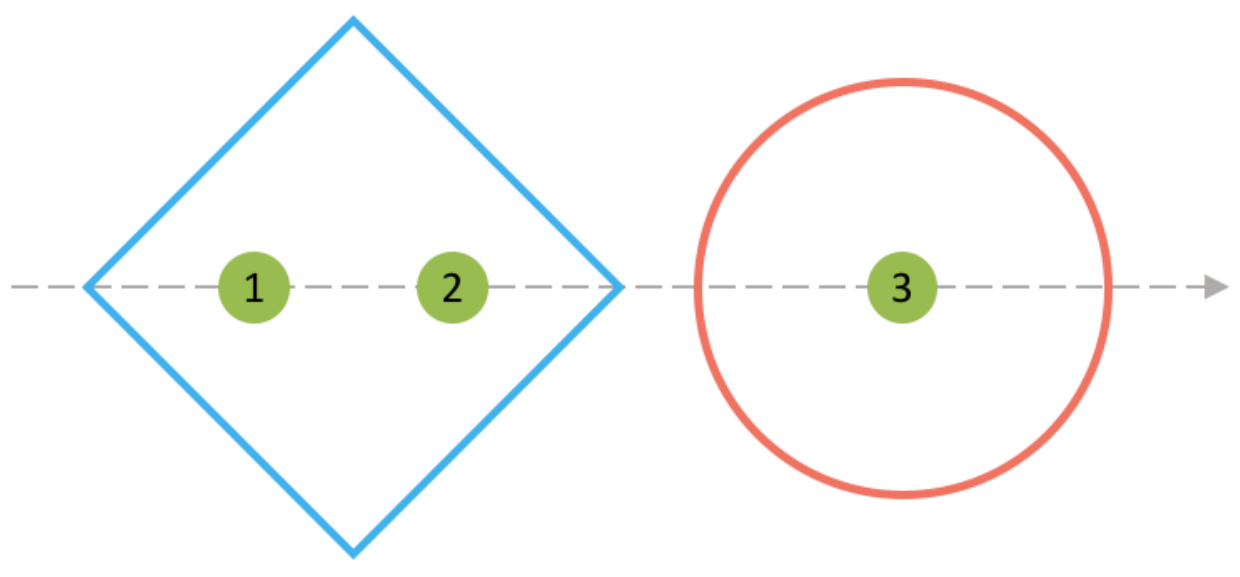
Under such an assumption, the last term of Eq. (27) becomes
| (83) |
where
| (84) |
is obtained from Eq. (12) by setting and . Note that for any value of and , which implies that also the coefficient in front of the double commutator in Eq. (83) is positive. Now, we express the position operators as sum of the center-of-mass position operator and relative position operator . In particular, in accordance with the division displayed in Fig. 5, we have for or 2; while for . Then, by tracing over the relative degrees of freedom [cf. Eq. (29)], Eq. (83) reduces to
| (85) | ||||
The last term of this equation is the additional term with respect to the original KTM model. The explicit expression of its coefficient is
| (86) |
which is always strictly positive, as noted above. This proves that such additional terms in general are non vanishing.
Appendix D The divergences and regularization in the TD model
The decoherence term (39) in the master equation (38) is only formally defined. We show that, under the assumption that is invariant under translations, i.e. , any choice of leads to divergences. To do so, let us consider a system of point-like particles, whose mass density is given by
| (87) |
By substituting it, once expressed in terms of its Fourier transform, in the decoherence term of Eq. (38), we obtain
| (88) | ||||
where is the Fourier transform of , which inherits the translational invariance from . Let us consider the terms in the above sum corresponding to the same particle (). These are proportional to
| (89) |
The first term diverges; a straightforward calculation show that according to Eq. (39):
| (90) |
where the Fourier transform of the inverse of the noise kernel is related to via Eq. (35):
| (91) |
Then, Eq. (90) can be written in terms of as
| (92) |
Equation (92) is the sum of two contributions: the continuous measurement, which gives the first term, and the application of the gravitational interaction through a feedback evolution, which provides the second term. Before analysing the general case, let us study two particular correlation kernels.
The first case corresponds to a LOCC dynamics, which requires that the dynamics acts only locally Tilloy and Diósi 2017. A noise correlation function reflecting this property is proportional to a Dirac-delta. Thus, we set
| (93) |
where is an arbitrary constant. In such a case, we have that . By substituting the latter expression in Eq. (92), one gets that none of its contributions is convergent. Thus, in the TD model, the assumptions of having point-like particles and implementing a LOCC dynamics lead to divergences.
As second case of interest, we consider a Gaussian correlation kernel . In this case, one has . Now, by substituting the latter expression in Eq. (92), we find that although the continuous measurement contribution converges, the feedback contribution is still divergent.
Next, we show the general case: any choice of leads to divergences. Similarly to what was done in the KTM model, we minimize the decoherence kernel with respect to . The minimum is reached for , which corresponds to . Such a correlation kernel leads to the decoherence rate of the Diósi-Penrose model Tilloy and Diósi 2017; Diósi 1989; Penrose 1996, which is still divergent Bahrami et al. 2014. Indeed, Eq. (92) in this case reads
| (94) |
Since the latter choice of provides the minimum decoherence rate, we deduce that Eq. (92), and subsequently the master equation (38), diverges for any choice of .
A regularization process is needed to avoid divergences in the decoherence terms in Eq. (38). This regularization mechanism is applied also to the Diósi-Penrose model Bahrami et al. 2014, by introducing a smearing function. For the TD model, the contributions to the decoherence term are those coming from the measurement part, through , and from the feedback evolution, through . Both these terms must be regularized. Indeed, the regularization of the noise kernel alone would only give a different noise kernel , which is not sufficient to avoid the divergence, as proved before. On the other hand, the regularization of the gravitational potential could remove the divergences in the feedback contribution, but not that due to the measurement, which is independent from the gravitational interaction. We conclude that the regularization mechanism must be performed by smearing both and .
An effective regularization procedure consists in smearing the mass density operator as proposed in Refs. Ghirardi et al. 1990; Tilloy and Diósi 2017. According to this prescription, we substitute the mass density with the smeared one
| (95) |
where is a suitable smearing function. This is equivalent to regularizing both the noise kernel and the gravitational potential with the same smearing function Tilloy and Diósi 2017:
| (96) |
An appropriate smearing function should remove all the divergences of the master equation (38) for an arbitrary choice of the mass density and of the noise kernel. In particular, in Eq. (30) becomes
| (97) |
and the decoherence kernel defined in Eq. (39) turns into
| (98) |
By substituting with and with in Eq. (38), we obtain
| (99) | ||||
In this way, we are able to retrieve a smeared quantum Newtonian gravitational interaction.
As a case of interest, we consider the noise correlation function by Eq. (93). In such a case, we obtain
| (100) | ||||
where we defined
| (101) |
with denoting the Fourier transform of . A good smearing function must give finite expressions in Eq. (100), which reflect an appropriate short-distance regularization of the Newtonian gravitational potential , the correlation kernel and the feedback dynamics . In turn, one can exploit Eq. (100) to restrict the class of smearing function. In particular, the requirement of the convergence of prevents the use of some intuitive choices for the smearing. Indeed, if one considers a Gaussian smearing , one has that both and converge, while , in spherical coordinates, becomes:
| (102) |
which diverges, since the integrand is not well defined for .
In the following, we determine the convergence requirements for the coefficients . For the sake of simplicity, we consider only spherical smearing functions, i.e. . In such a case, Eq. (101) simplifies to
| (103) |
which converges, for example, for smearing functions of the family with and . Concretely, a smearing function of the form
| (104) |
whose Fourier transform is
| (105) |
belongs to such a family. In particular, explicit calculations lead to
| (106) | ||||
which are well defined also for . In this way, the divergences in the TD model are indeed avoided.
If instead of Eq. (93), one takes , a normalized Gaussian smearing of standard deviation leads to the following a decoherence kernel
| (107) |
which behaves well also for .
References
- Tosto (2012) S. Tosto, Prog. Phys. 2, 58 (2012).
- Abbott et al. (2016) B. P. Abbott et al. (LIGO Scientific Collaboration and Virgo Collaboration), Phys. Rev. Lett. 116, 061102 (2016).
- Peebles and Ratra (2003) P. J. E. Peebles and B. Ratra, Rev. Mod. Phys. 75, 559 (2003).
- Barack et al. (2019) L. Barack et al., Class. Quantum Grav. 36, 143001 (2019).
- Kiefer (2007) C. Kiefer, Quantum Gravity (Oxford University Press, 2007).
- Hossenfelder (2011) S. Hossenfelder, “Classical and quantum gravity: Theory, analysis and applications,” (Nova Publishers, 2011) Chap. Experimental Search for Quantum Gravity, pp. 257–282.
- Feynman (1995) R. P. Feynman, “Feynman lectures on gravitation,” (Addison-Wesley, 1995) Chap. On the philosophical problems in quantizing macroscopic objects, pp. 11–15.
- (8) L. Diósi, N. Gisin, and W. T. Strunz, Phys. Rev. A 61, 022108.
- Carlip (2001) S. Carlip, Rep. Prog. Phys. 64, 885 (2001).
- Huggett and Callender (2001) N. Huggett and C. Callender, Philos. Sci. 68, S382 (2001).
- Peres and Terno (2001) A. Peres and D. R. Terno, Phys. Rev. A 63, 022101 (2001).
- Wüthrich (2005) C. Wüthrich, Philos. Sci. 72, 777 (2005).
- Rothman and Boughn (2006) T. Rothman and S. Boughn, Found. Phys. 36, 1801 (2006).
- Carlip (2008) S. Carlip, Class. Quantum Grav. 25, 154010 (2008).
- Dyson (2013) F. Dyson, Int. J. Mod. Phys. A 28, 1330041 (2013).
- Ahmadzadegan et al. (2016) A. Ahmadzadegan, R. B. Mann, and D. R. Terno, Phys. Rev. A 93, 032122 (2016).
- Bassi et al. (2017) A. Bassi, A. Großardt, and H. Ulbricht, Class. Quantum Grav. 34, 193002 (2017).
- Tilloy (2018a) A. Tilloy, Found. Phys. 48, 1753 (2018a).
- Carney et al. (2019) D. Carney, P. C. E. Stamp, and J. M. Taylor, Class. Quantum Grav. 36, 034001 (2019).
- Kumar and Plenio (2020) S. P. Kumar and M. B. Plenio, Nat. Commun. 11, 3900 (2020).
- Donadi et al. (2020) S. Donadi, K. Piscicchia, C. Curceanu, L. Diósi, M. Laubenstein, and A. Bassi, Nat. Phys. (2020).
- Diósi (1989) L. Diósi, Phys. Rev. A 40, 1165 (1989).
- Penrose (1996) R. Penrose, Gen. Rel. Grav. 28, 581 (1996).
- Diósi (2011) L. Diósi, J. Phys. Conf. Ser. 306, 012006 (2011).
- Bowen and Milburn (2016) W. P. Bowen and G. J. Milburn, Quantum Optomechanics (CRC Press, 2016).
- Khosla and Altamirano (2017) K. E. Khosla and N. Altamirano, Phys. Rev. A 95, 052116 (2017).
- Altamirano et al. (2017a) N. Altamirano, P. Corona-Ugalde, K. E. Khosla, G. J. Milburn, and R. B. Mann, Class. Quantum Grav. 34, 115007 (2017a).
- Khosla and Nimmrichter (2018) K. E. Khosla and S. Nimmrichter, ArXiv 1812.03118 (2018).
- Altamirano et al. (2018) N. Altamirano, P. Corona-Ugalde, R. B. Mann, and M. Zych, Class. Quantum Grav. 35, 145005 (2018).
- Tilloy (2018b) A. Tilloy, Phys. Rev. D 97, 021502 (2018b).
- Tilloy (2019) A. Tilloy, J. Phys.: Conf. Ser. 1275, 012006 (2019).
- Kafri et al. (2014) D. Kafri, J. M. Taylor, and G. J. Milburn, New J. Phys. 16, 065020 (2014).
- Tilloy and Diósi (2017) A. Tilloy and L. Diósi, Phys. Rev. D 96, 104045 (2017).
- Kafri et al. (2015) D. Kafri, G. J. Milburn, and J. M. Taylor, New J. Phys. 17, 015006 (2015).
- Jacobs (2014) K. Jacobs, Quantum Measurement Theory and its Applications (Cambridge University Press, 2014).
- Benenti et al. (2019) G. Benenti, G. Casati, D. Rossini, and G. Strini, Principles of Quantum Computation and Information (A Comprehensive Textbook) (World Scientific, 2019).
- Koashi (2016) M. Koashi, “Principle and methods of quantum information technologies,” (Springer, 2016) Chap. Quantum Information Theory for Quantum Communication, pp. 3–33.
- Chitambar et al. (2014) E. Chitambar, D. Leung, L. Mančinska, M. Ozols, and A. Winter, Comm. Math. Phys. 328, 303 (2014).
- Marshman et al. (2020) R. J. Marshman, A. Mazumdar, and S. Bose, Phys. Rev. A 101, 052110 (2020).
- Horodecki et al. (2009) R. Horodecki, P. Horodecki, M. Horodecki, and K. Horodecki, Rev. Mod. Phys. 81, 865 (2009).
- Altamirano et al. (2017b) N. Altamirano, P. Corona-Ugalde, R. B. Mann, and M. Zych, New J. Phys. 19, 013035 (2017b).
- Kovachy et al. (2015) T. Kovachy, P. Asenbaum, C. Overstreet, C. A. Donnelly, S. M. Dickerson, A. Sugarbaker, J. M. Hogan, and M. A. Kasevich, Nature 528, 530 (2015).
- Tilloy and Diósi (2016) A. Tilloy and L. Diósi, Phys. Rev. D 93, 024026 (2016).
- Diósi and Tilloy (2017) L. Diósi and A. Tilloy, Open Systems & Information Dynamics 24, 1740020 (2017).
- Jacobs and Steck (2006) K. Jacobs and D. A. Steck, Contemp. Phys. 47, 279 (2006).
- Wiseman and Milburn (1993) H. M. Wiseman and G. J. Milburn, Phys. Rev. Lett. 70, 548 (1993).
- Wiseman and Milburn (2010) H. M. Wiseman and G. J. Milburn, Quantum Measurement and Control (Cambridge University Press, 2010).
- Zhang et al. (2017) J. Zhang, Y. xi Liu, R.-B. Wu, K. Jacobs, and F. Nori, Phys. Rep. 679, 1 (2017).
- Diósi and Gisin (1994) L. Diósi and N. Gisin, Phys. Rev. Lett. 72, 4053 (1994).
- Ulmer and Kaissl (2003) W. Ulmer and W. Kaissl, Phys. Med. Biol. 48, 707 (2003).
- Bahrami et al. (2014) M. Bahrami, A. Smirne, and A. Bassi, Phys. Rev. A 90, 062105 (2014).
- Ghirardi et al. (1990) G. Ghirardi, R. Grassi, and A. Rimini, Phys. Rev. A 42, 1057 (1990).