An Experimental mmWave Channel Model
for UAV-to-UAV CommunicationsConference: 4th ACM Workshop on Millimeter-wave Networks and Sensing Systems; September 25, 2020; London, UK4th ACM Workshop on Millimeter-wave Networks and Sensing Systems (mmNets’20), September 25, 2020, London, UKPrice: 15.00DOI: 10.1145/xxxxxxx.xxxxxxxxISBN: xxxxxxxxxxxxxxxxxxxxxxxxx
Abstract.
Unmanned Aerial Vehicle (UAV) networks can provide a resilient communication infrastructure to enhance terrestrial networks in case of traffic spikes or disaster scenarios. However, to be able to do so, they need to be based on high-bandwidth wireless technologies for both radio access and backhaul. With this respect, the millimeter wave (mmWave) spectrum represents an enticing solution, since it provides large chunks of untapped spectrum that can enable ultra-high data-rates for aerial platforms. Aerial mmWave channels, however, experience characteristics that are significantly different from terrestrial deployments in the same frequency bands. As of today, mmWave aerial channels have not been extensively studied and modeled. Specifically, the combination of UAV micro-mobility (because of imprecisions in the control loop, and external factors including wind) and the highly directional mmWave transmissions require ad hoc models to accurately capture the performance of UAV deployments. To fill this gap, we propose an empirical propagation loss model for UAV-to-UAV communications at , based on an extensive aerial measurement campaign conducted with the Facebook Terragraph channel sounders. We compare it with 3GPP channel models and make the measurement dataset publicly available.
Keywords:
mmWave, UAV, Cellular Networks, 60 GHz, Propagation.1. Introduction
Unmanned aerial systems are promising technological enablers for the wireless industry, as they provide an effective and inexpensive solution to temporarily connect ground users in the absence of terrestrial infrastructure (Bertizzolo et al. 2020a; Bertizzolo et al. 2020b; Bertizzolo et al. 2019). In this domain, a key research challenge is how to provide high-capacity robust backhaul and inter-Unmanned Aerial Vehicle (UAV) connectivity in flying platforms. Fiber optic backhaul, typical of terrestrial infrastructure, is not a feasible solution for UAVs, thus, both the radio access and the backhaul exploit wireless links.
However, combining access and backhaul on the same wireless interface introduces tight data-rate and latency requirements to the underlying communication technology. This problem is exacerbated when multiple UAVs rely on each other for data forwarding, in an aerial multi-hop fashion. While traditional sub- technologies are unfit for high-load traffic aggregation, the millimeter wave (mmWave) spectrum can be a unified solution for fully-wireless nodes offering unprecedented bandwidth. Thus, at mmWaves, a UAV network can use the same wireless technology to provide connectivity to ground users, communicate with neighboring UAVs, and relay data traffic toward the closest ground tower, in an “integrated access and backhaul” fashion (Polese et al. 2020).
Even though recent 5G standard specifications already envision the use of mmWaves (3GPP 2018a), and some previous work studied their propagation for ground deployments (Rappaport et al. 2017; 3GPP 2018b), the aerial wireless channel at mmWave frequencies has not been extensively characterized yet. Indeed, mmWaves may affect the communication quality in aerial scenarios differently from ground deployments, for the following reasons: (i) Some frequencies in the mmWave spectrum (e.g., the 60 GHz band) suffer from oxygen absorption. As these atmospheric conditions change with the deployment height, high-altitude aerial scenarios might differ from ground deployments; (ii) even when Global Positioning System (GPS)-locked, the inaccuracy of UAV’s on-board sensors may lead to slight horizontal (yaw) and vertical (throttle) drone fluctuations. Given that mmWaves exploit highly directional communications, these fluctuations might severely deteriorate the channel quality (Bertizzolo et al. 2019); (iii) when UAVs fly in harsh wind conditions, they lean forward/backward (pitch) and sideways (roll) to counterbalance the wind force. Tilting a UAV-mounted mmWave radio might compromise the link quality by changing the best beam path or the radios’ polarization (Khuwaja et al. 2018); (iv) on-board mmWave radios are often mounted either above or below the main UAV’s frame structure. The frame size and its material, together with the spinning propellers introduce ambient noise right where the headset is mounted. On-board batteries, radio control, and circuitry non-linearity exacerbate this effect known as “airframe shadowing” (Semkin et al. 2020). For these reasons, the performance evaluation of mmWave UAV-to-UAV communications cannot be based upon ground-tailored mmWave channel studies and demands the development of dedicated air-to-air (A2A) propagation and fading models. Prior work has focused on analytical or ray-tracing approaches (Khawaja et al. 2017; Khawaja et al. 2018; Gapeyenko et al. 2018; Dabiri et al. 2020), which have not been validated through experimental measurement campaigns.
In this paper, we propose an empirical propagation loss model for A2A communications at . It is based on an extensive measurement campaign, with more than 3 days of flight experiments, and the Facebook Terragraph channel sounders (Facebook 2019) mounted on two UAVs. The measurements validate the empirical model in a wide range of flying heights () and distances (), and show that, in the considered range, the path loss does not have an explicit dependence on the UAV height. Moreover, we compare the path loss curve with 3GPP channel models, and, using the same measurement campaign, we characterize the impact of a sub-optimal beam selection on the link budget. To the best of our knowledge, this is the first empirical A2A propagation model for the 60 GHz band modeling the impact of the UAVs micro-mobility on the channel. Last, we publicly release the collected measurements’ dataset and analysis scripts to the community.11 1 https://github.com/wineslab/uav-to-uav-60-ghz-channel-model
The remainder of the paper is organized as follows. Sec. 2 describes the measurement campaign. Sec. 3 analyzes empirical path loss fits on the collected data and compares them with terrestrial channel models. Finally, Sec. 4 concludes the paper.

2. Measurement Campaign Setup
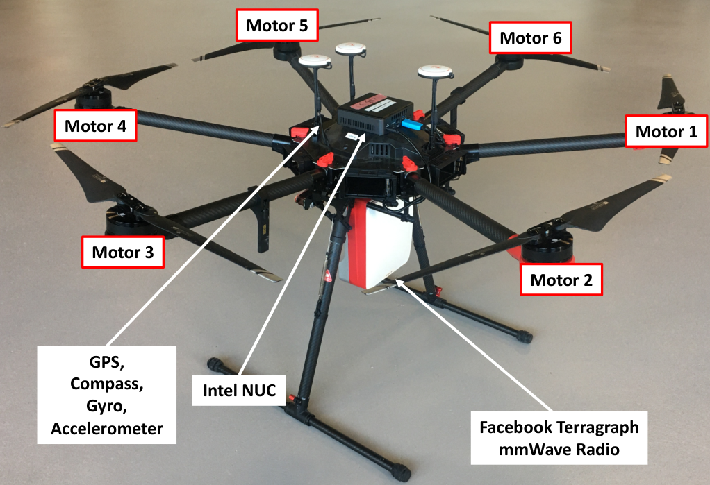
For our measurements, we employed two DJI M as UAVs and two Facebook Terragraph mmWave radios configured as channel sounders with beam scanning capabilities. Each DJI M mounts an on-board powered Intel NUC computer to perform flight control tasks, while the Facebook Terragraph radios are powered from the ground and coordinated in their channel sounding procedures by a ground host controller. The hardware and software schematics of the mmWave-enabled UAV are reported in Fig. 1.
The Facebook Terragraph channel sounders operate in the IEEE 802.11ad bands (Telecom Infra Project 2019a). The radios feature TX and RX arrays of antenna elements with an angular coverage of and beam directions in the azimuth plane, thus with a spacing between each beam of . The half-power beamwidth is , and the radio maximum effective radiated power is . Moreover, the antenna, circuitry, and main board are enclosed in a rugged case, with a small weight and form factor that makes it possible to deploy them on UAVs. Facebook Terragraph sounders have recently been used for channel measurement campaigns in the band by several research groups. They are calibrated following the procedure in (Telecom Infra Project 2019a) and allow received power, path loss, and Signal to Noise Ratio (SNR) measurements for different transmit and receive beam pairs. The standard deviation in path loss measurements within 1 dB (Telecom Infra Project 2019a). Some of Facebook Terragraph previous use and documentation can be found at (Bertizzolo et al. 2019; Rasekh et al. 2017; Telecom Infra Project 2019b; Telecom Infra Project 2019a; Telecom Infra Project 2019c).
In our measurement campaign, we run extensive channel sounding experiments on a wide open field with few reflectors and scarce multi-path effect as illustrated in Fig. 2.22 2 A video of the experiments is available at https://youtu.be/Jzwt-tEp98g. For each experiment, the transmitter and receiver UAVs hover at the same altitude and face each other in full Line of Sight (LOS) conditions. Through our experiment, we consider heights, , , and ; and a total of distances between transmitter and receiver, namely 6, 9, 12, 15, 18, 21, 24, 27, 28, 30, 32, 33, 36, and , as shown in Fig. 2. The selection of these coordinates has been constrained by the size of the UAV flying facility. We performed channel measurements for channel of the IEEE 802.11ad standard (i.e., the carrier frequency is , and the bandwidth if ) and altitude-distance pairs, accounting for 3 days of flight experiments. Each channel sounding experiment consists of scanning the beam pairs, between from the boresight direction (see (Telecom Infra Project 2019a) for specifications), with independent measurements per beam scan, to average small scale fading, and a distance-adaptive transmission gain.

3. Path Loss Analysis
This section describes the data analysis based on the measurement campaign outlined in Sec. 2.
3.1. Experimental Path Loss Laws
The literature on propagation models has proposed several experimental path loss laws that can be used to fit the measurement results as a function of distance and frequency parameters. A review can be found in (Rappaport et al. 2017). In this paper, as the measurements have been taken for a single carrier frequency (i.e., 60.48 GHz), we focus on a distance-dependent fit only.
The Close-in free space reference (CI) path loss models can be expressed as (Rappaport et al. 2017)
| (1) |
The first term, , is used to model the dependence on the carrier frequency, and is calculated using Friis’ law for free space propagation, at the reference distance of 1 m (Sun et al. 2015):
| (2) |
where is the speed of light. The second term accounts for the logarithmic distance-dependent behavior, with the path loss exponent (PLE), given by the value that best fits the measurement data. Finally, is a shadow fading term that in the decibel domain follows a Gaussian distribution with zero mean and standard deviation . The CI model is widely used for empirical path loss fitting, either in the single-slope version of Eq. (1) (Rappaport et al. 2017; 3GPP 2018b), or with a dual-slope extension, in which different values of are considered before and after a breakpoint distance (3GPP 2018b; white paper 2016).
Other widespread models belong to the Floating Intercept (FI) family, in which the term based on Friis’ law is replaced by a generic value, determined based on the best fit on the data. A notable example is the Alpha-Beta-Gamma (ABG) model, given by (Rappaport et al. 2017)
| (3) |
where is a Gaussian shadow fading with zero mean and standard deviation , as in the CI model, and , , and are fit on the data. With respect to the CI model in Eq. (1), the term is equivalent to the path loss exponent . Notice that, as the measurement campaign of this paper is based on a single frequency, we cannot compute both and . Therefore, in the following, we will consider a simplified version, with two fit parameters, given by
| (4) |
where , , and .
For both models, the fit parameters (i.e., for CI, and and for FI) are computed as the slope (and the intercept, for FI) of a linear fit on the logarithm of the distance, and the standard deviation of the shadow fading is computed as the root mean square error on the fit (Rappaport et al. 2017; Amorim et al. 2017).
3.2. Comparison of CI and FI Fits
We first discuss whether a CI fit is representative of the A2A path loss measurements, or whether a FI fit is preferable. Figure 3 compares the two methods, considering data for all the values for the height (i.e., m) and distance from to . Both curves share the same trend, with the FI fit slightly steeper, but with a difference of at most at and at . Table 3 reports the fit parameters for both, showing that the FI identifies a fit for its floating intercept at a , which is smaller than the free space path loss in the same conditions, and a path loss exponent of , against the value of for the CI fit. The shadowing standard deviation is smaller for the FI fit, which is almost two orders of magnitude smaller than the actual value of (i.e., for FI and for CI). Following standard practices in the literature (Sun et al. 2015), we conclude that both models provide a suitable representation of the path loss in a A2A link. Given this, in the remainder of the paper, we will consider the CI fit as baseline, as it is simpler than the FI fit (i.e., one fit parameter instead of two), and is based on the fundamental principles of wireless propagation through the Friis-based intercept (Sun et al. 2015).
| Intercept [dB] | Path loss exponent | [dB] | |
|---|---|---|---|
| CI fit | 68.08 | 2.25 | 3.56 |
| FI fit | 67.03 | 2.33 | 3.52 |
3.3. Impact of the Height on Path Loss
| All heights | m | m | m | |
|---|---|---|---|---|
| PLE | 2.25 | 2.23 | 2.25 | 2.28 |
| [dB] | 3.56 | 0.82 | 2.62 | 8.06 |
As the deployment height of UAV networks is subject to application scenario, regulations, and performance requirements (Amorim et al. 2017), it is important to characterize the channel behavior for a wide range of deployment heights. Therefore, in Fig. 4 we investigate the impact of the height on the parameters of a CI fit. For this, we consider separate CI fits for the three values of the UAVs height at which the measurements were collected, i.e., , , and , and compare them with a CI fit that does not distinguish between different heights. As can be seen, the four curves in Fig. 4 share the same trend, with differences of less than 1 dB between the curves for m and m in the worst case. The path loss exponent and the standard deviation are shown in Table 2. The value of is very similar for the four fits, showing that the height does not a significant impact once the UAVs are in flight. The standard deviation shows a higher variability, also with respect to the FI fit previously described, but this can be traced back to the fewer measurements considered for the fit at each single height value.
3.4. Comparison with Free Space and 3GPP Path Loss Models
| Best beam pair | 2nd best | 3rd best | 4th best | 5th best | 6th best | 7th best | 8th best | 9th best | |
|---|---|---|---|---|---|---|---|---|---|
| PLE | 2.25 | 2.28 | 2.07 | 1.96 | 2.01 | 1.93 | 1.99 | 2.02 | 2.03 |
| Intercept [dB] | 68.08 | 69.68 | 74.10 | 76.79 | 77.26 | 79.31 | 79.35 | 79.52 | 79.73 |
| [dB] | 3.56 | 3.78 | 4.85 | 4.61 | 4.01 | 5.76 | 5.80 | 5.38 | 4.82 |
| Displacement [deg] | 0 | 1.87 | 2.59 | 2.70 | 3.47 | 3.42 | 4.20 | 3.89 | 4.20 |
As discussed in Sec. 1, aerial communications are affected by a different channel than terrestrial networks, where both endpoints are on the ground and present less erratic mobility patterns. An aerial link is indeed characterized by a particularly strong LOS link, while reflections provide limited or no contribution, as scatterers are at a larger distance than in cellular or indoor scenarios. Furthermore, the micro-mobility of the UAVs, given by the fluctuations caused by the UAV control loop and/or wind conditions, may degrade the link quality (Dabiri et al. 2020).
Figure 5 shows that the measurement-based fit we propose in this paper reflects these phenomena into a higher path loss exponent with respect to free space path loss and of 3rd Generation Partnership Project (3GPP) channel models. We consider the equations for LOS propagation loss from the 3GPP channel model for frequencies between 0.5 and 100 GHz (3GPP 2018b), with an additional distance-dependent oxygen absorption loss factor for the 60 GHz band. We compare the path loss of different 3GPP scenarios, i.e., for Rural Macro (RMa), Urban Macro (UMa), Urban Micro (UMi) and Indoor Open Office (InOo) deployments. The free space path loss follows Friis’ law (Rappaport et al. 2017). The path loss curves in Fig. 5 confirm that the propagation of 60 GHz signals experiences a higher loss in an aerial link, as it has a path loss exponent which is larger than the worse LOS exponent in 3GPP scenarios (i.e., 2.1 for UMi). This confirms that the analysis and simulation of aerial networks cannot be based on channel models developed for terrestrial applications, and motivates the development of the experimental channel model proposed in this paper.
3.5. Path Loss Curves with Misalignment
mmWave links will rely on beamforming techniques to increase the link budget and compensate for the increased path loss. In this sense, a proper beam alignment makes it possible to select the transmit and receive beams that yield the highest beamforming gain. Fast and prompt beam tracking, however, can be challenging in aerial links, where the nodes are highly mobile (Bertizzolo et al. 2019). Therefore, we present in the following paragraph the path loss curves that fit measurements for beam pairs that are not perfectly aligned, following a similar approach discussed in (Priebe et al. 2012) for terahertz links. Notice that these results do not represent the actual path loss (which is given only by the data for the best beam pair), but are a practical way to model the loss in beamforming gain due to misalignment.
For this analysis, we exploit the beam scanning capabilities of the Terragraph channel sounders (Telecom Infra Project 2019a). For each distance and height at which measurements are taken, the beam pair that yields the lowest path loss is considered for the CI fit previously described. We then analyze the remaining beam pairs, and, for each distance-height point, select the second-through-ninth best beam pairs in terms of path loss. Finally, we apply an FI fit for each of these, by aggregating the data for different heights. For this analysis, the FI fit is preferred over the CI fit, as its intercept term allows the modeling of the additional loss (with respect to the free space path loss) introduced by beam misalignment.
As an example, Fig. 6 reports the measurements and fitted path loss curves for the second, third and ninth-best beam pairs, and the path loss curve for the best beam pair. We observe that the distance between measured points and the best beam pair fit line progressively increases, as the misalignment between the non-optimal beam pairs decreases the beamforming gain. Figure 7, instead, directly compares path loss curves, which exhibit the same trend, as the physical path loss between the two nodes does not change, but have an increasing loss factor that models the reduction in beamforming gain.
To further underline this, we list in Table 3 the path loss exponents, which are comparable for the different beam pairs, and the intercept values, which increase by up to from the best to the ninth-best beam pair. We also provide a displacement metric, to model the angular error that can lead to such loss in beamforming gain. Notably, for the -th-best beam pair, , we have , with the average operator, and and the angles of the best beam, and of the beam associated to the -th beam pair, for , respectively. As discussed in Sec. 2, the beams of the Terragraph sounders are spaced by . Therefore, , for the second beam pair, suggests that, on average, the beamforming gain loss is due to a misalignment of 1.33 beam pairs, either at the receiver or the transmitter. We notice that saturates after the fifth-best beam pair, and that the intercept has a limited difference, showing that the misalignment is likely due to the selection of equivalent beam pairs.
4. Conclusions
In this paper, we described an extensive measurement campaign for the characterization of the A2A path loss at , using the Facebook Terragraph radios configured as channel sounders. The data analysis led us to conclude that the propagation loss of an aerial link, for heights between and , is well represented by the equation:
| (5) |
with a Gaussian random variable with standard deviation dB. Moreover, we compared this fit with established propagation models for mmWaves, and analyzed the impact of a sub-optimal beam selection on the link performance. For this case, the combined path loss and gain reduction can be computed using Eq. (4) with the parameters from Table 3.
As part of our future work, we will extend the validation of the path loss curves by performing measurements in different scenarios and with different sounders, and analyze the impact of beam misalignment with different beamforming configurations, as well as of the Doppler effect in highly mobile conditions. Moreover, we will characterize air-to-ground (A2G) mmWave channels and extend the height range for the A2A measurements.
Acknowledgements
This work was supported in part by the US National Science Foundation under Grant CNS-1618727 and in part by the US Office of Naval Research under Grants N00014-19-1-2409 and N00014-20-1-2132.
References
- (1)
- 3GPP (2018a) 3GPP. 2018a. NR; Overall description; Stage-2. Technical Specification (TS) 38.300. Version 15.0.0.
- 3GPP (2018b) 3GPP. 2018b. Study on channel model for frequencies from 0.5 to 100 GHz. Technical Report (TR) 38.901. Version 15.0.0.
- Amorim et al. (2017) R. Amorim, H. Nguyen, P. Mogensen, I. Z. Kovács, J. Wigard, and T. B. Sørensen. 2017. Radio Channel Modeling for UAV Communication Over Cellular Networks. IEEE Wireless Communications Letters 6, 4 (Aug 2017), 514–517. https://doi.org/10.1109/LWC.2017.2710045
- Bertizzolo et al. (2020a) L. Bertizzolo, S. D’oro, L. Ferranti, L. Bonati, E. Demirors, Z. Guan, T. Melodia, and S. Pudlewski. 2020a. SwarmControl: An Automated Distributed Control Framework for Self-Optimizing Drone Networks. In Proc. of IEEE Conf. on Computer Communications (INFOCOM).
- Bertizzolo et al. (2019) L. Bertizzolo, M. Polese, L. Bonati, A. Gosain, M. Zorzi, and T. Melodia. 2019. mmBAC: Location- aided mmWave Backhaul Management for UAV-based Aerial Cells. In Proc. of 3rd ACM Workshop on Millimeter-wave Networks and Sensing Systems (mmNets). Los Cabos, Mexico.
- Bertizzolo et al. (2020b) L. Bertizzolo, T. X. Tran, B. Amento, B. Balasubramanian, R. Jana, H. Purdy, Y. Zhou, and T. Melodia. 2020b. Live and Let Live: Flying UAVs Without Affecting Terrestrial UEs. In Proc. of the 21st Intl. Workshop on Mobile Comput. Systems and Appl. (HotMobile). Austin, TX, USA.
- Dabiri et al. (2020) M. T. Dabiri, H. Safi, S. Parsaeefard, and W. Saad. 2020. Analytical Channel Models for Millimeter Wave UAV Networks Under Hovering Fluctuations. IEEE Trans. Wireless Commun. 19, 4 (Feb 2020), 2868–2883.
- Facebook (2019) Terragraph Facebook. 2019. https://terragraph.com/product.
- Gapeyenko et al. (2018) M. Gapeyenko, V. Petrov, D. Moltchanov, S. Andreev, N. Himayat, and Y. Koucheryavy. 2018. Flexible and Reliable UAV-Assisted Backhaul Operation in 5G mmWave Cellular Networks. IEEE J. Sel. Areas Commun. 36, 11 (Nov 2018), 2486–2496.
- Khawaja et al. (2017) W. Khawaja, O. Ozdemir, and I. Guvenc. 2017. UAV Air-to-Ground Channel Characterization for mmWave Systems. In Proc. of IEEE VTC-Fall. Toronto, ON, Canada.
- Khawaja et al. (2018) W. Khawaja, O. Ozdemir, and I. Guvenc. 2018. Temporal and Spatial Characteristics of mmWave Propagation Channels for UAVs. In Proc. of IEEE Global Symp. on Millimeter Waves (GSMM). Boulder, CO, USA.
- Khuwaja et al. (2018) A. A. Khuwaja, Y. Chen, N. Zhao, M. Alouini, and P. Dobbins. 2018. A Survey of Channel Modeling for UAV Communications. IEEE Commun. Surveys Tuts. 20, 4 (Fourth quarter 2018), 2804–2821.
- Polese et al. (2020) M. Polese, M. Giordani, T. Zugno, A. Roy, S. Goyal, D. Castor, and M. Zorzi. 2020. Integrated Access and Backhaul in 5G mmWave Networks: Potential and Challenges. IEEE Commun. Mag. 58, 3 (Mar 2020), 62–68.
- Priebe et al. (2012) S. Priebe, M. Jacob, and T. Kürner. 2012. Affection of THz indoor communication links by antenna misalignment. In Proc. of 6th European Conf. on Antennas and Propagation (EUCAP). Prague, Czech Republic, 483–487. https://doi.org/10.1109/EuCAP.2012.6206026
- Rappaport et al. (2017) T. S. Rappaport, Y. Xing, G. R. MacCartney, A. F. Molisch, E. Mellios, and J. Zhang. 2017. Overview of Millimeter Wave Communications for Fifth-Generation (5G) Wireless Networks—With a Focus on Propagation Models. IEEE Trans. Antennas Propag. 65, 12 (Dec 2017), 6213–6230.
- Rasekh et al. (2017) Maryam Eslami Rasekh, Zhinus Marzi, Yanzi Zhu, Upamanyu Madhow, and Haitao Zheng. 2017. Noncoherent mmWave path tracking. In Proc. of the 18th Intl. Workshop on Mobile Computing Systems and Applications. Sonoma, CA, USA, 13–18.
- Semkin et al. (2020) V. Semkin, J. Haarla, T. Pairon, C. Slezak, S. Rangan, V. Viikari, and C. Oestges. 2020. Analyzing Radar Cross Section Signatures of Diverse Drone Models at mmWave Frequencies. IEEE Access 8 (Mar 2020), 48958–48969.
- Sun et al. (2015) S. Sun, T. A. Thomas, T. S. Rappaport, H. Nguyen, I. Z. Kovacs, and I. Rodriguez. 2015. Path Loss, Shadow Fading, and Line-of-Sight Probability Models for 5G Urban Macro-Cellular Scenarios. In Proc. of IEEE Globecom Workshops (GC Wkshps). 1–7.
- Telecom Infra Project (2019a) Telecom Infra Project. 2019a. Analysis of 28GHz and 60GHz Channel Measurements in an Indoor Environment. https://tinyurl.com/y6uk25ej
- Telecom Infra Project (2019b) Telecom Infra Project. 2019b. mmWave Measurement Campaign using Terragraph Channel Sounders. https://tinyurl.com/yawgbgbx
- Telecom Infra Project (2019c) Telecom Infra Project. 2019c. Study of mmWave Signal Propagation in Non-line-of-sight Environment. https://tinyurl.com/y7rckdhx
- white paper (2016) 5GCM white paper. 2016. 5G channel model for bands up to 100 GHz. https://tinyurl.com/y3oo8kmb