Graphs isomorphisms under edge-replacements
and the family of amoebas

Graphs called amoebas first appeared in [12] where certain Ramsey-Turán extremal problems were considered, which dealt with the existence of a given graph with a prescribed color pattern in $2$-edge-colorings of the complete graph. More precisely, amoebas arose from the search of a graph family with certain interpolation properties that could be suitable to show balanceability or omnitonal properties [12] (see also [11]). The graphs named just “amoebas” in [12] are called in this paper, with their rich, Matroid resembling properties, “global amoebas”, as we will distinguish them from a similar family that we call “local amoebas”. For the interested reader, we refer to [6, 22, 23, 32, 36, 37, 44] for more literature related to interpolation techniques in graphs.

The feature that makes amoebas work are one-by-one replacements of edges, where, at each step, some edge is substituted by another such that an isomorphic copy of the graph is created. We call such edge substitutions feasible edge-replacements. Similar edge-operations have been studied, for instance, in [13, 18, 19, 28, 37, 39]. As introduced in [11], a family $\mathcal{F}$ of graphs, all of them having the same number of edges, is called closed in a graph $H$ if, for every two copies $F,F^{\prime}$ of members of $\mathcal{F}$ contained in $H$, there is a chain of graphs $H_{1},H_{2},\ldots,H_{k}$ in $H$ such that $H_{1}\cong F$, $H_{k}\cong F^{\prime}$, and, for $2\leq i\leq k$, $H_{i}$ is isomorphic to a member of $\mathcal{F}$ and $H_{i}$ is obtained from $H_{i-1}$ by interchanging one edge with another (an edge-replacement that is not necessarily feasible). Perhaps the most well-known closed family is the family of all spanning trees of a connected graph $H$, and the edge-replacement operation given above is in fact the basic operation in the exchange of bases in the cycle matroid $M(H)$ of $H$. A graph $G$ is a global amoeba precisely when $\{G\}$ is a closed family in $K_{n}$ (for $n$ large enough), and it is a local amoeba if $\{G\}$ is a closed family in $K_{n(G)}$. Exactly this global amoeba property is the key to the usefulness of amoebas in interpolation theorems in Graph Theory and in zero-sum extremal problems [11], and in problems about forced patterns in $2$-colorings of the edges of $K_{n}$ [12]. We note at this point, once again, that the amoebas defined in [12] correspond to the class of global amoebas.

A first encounter with amoebas gives the impression that such graphs are very rare and have a very simple structure. This, however, is not the case and amoebas may have quite a complicated structure. Indeed, we will consider here different constructions with which we will show that any connected graph can be a connected component of a global amoeba (Theorem 5.7), that global amoebas can be very dense (in fact, with as many as $n^{2}/4$ edges, being $n$ the order of the graph) and, that they can have very large chromatic number and cliques, too (as large as roughly half the order of the graph) (Theorem 6.1). Also, we introduce an interesting family of global amoeba trees with a Fibonacci-like structure and with arbitrary large maximum degree (Theorem 5.12).

Most concepts and definitions concerning amoebas can be stated in graph theoretical language. However, a group theoretical setting with which the dynamics of the edge replacements are modeled – and which involve graph isomorphisms – will be necessary for proving several results. In particular, the proof of Theorem 3.8, which is a key element for many other results, employs tools of permutation groups, which via graph theoretical language would be too intricate. This is the reason why we will develop an algebraic theoretical setting so that we can then formalize all concepts and definitions by means of the permutation language, and we will proceed further on with the theory this way. The research on amoebas is related to problems like switching in graphs [5, 25], reconfiguration problems [27, 35], token graphs [9, 17, 31] and, with respect to aspects of group action language, to reconstruction problems in graphs [15, 24, 30]. Similar approaches that deal with graph isomorphisms can be found in [1, 38, 40]. For group theoretical concepts, we refer to [26].

The paper is organized as follows. In Section 2, we define local and global amoebas formally by means of graph theoretical language, and present some basic results achievable by graph theoretical tools. In Section 3, we introduce the group theoretical tools that will let us model how the so-called feasible edge-replacements work via permutations. By means of this algebraic setting, we will reformulate the definitions of global amoeba and local amoeba (Definition 3.2). Section 4 contains our main result (Theorem 4.1) which displays different characterizations of global amoebas by which the relation between global and local amoebas is very clearly established. Moreover, it is shown, using non-trivial examples, how the characterization is very handy. In Section 5, we will present some interesting constructions of both local and global amoebas that will exhibit the richness of this family of graphs.

For many of these results, Theorem 4.1 is a crucial tool. In Section 6, we exhibit extremal global amoebas with respect to size, chromatic number and clique number. In order to show the purpose of the results, we will illustrate with abundant examples. In the final section, we provide the reader with several open problems which could bring more light to understanding this very interesting family of graphs called amoebas. Figure 1 depicts a scheme that captures the structure and the dependence between the results of this paper. The scheme includes Definition 3.2 to emphasize that the developed theory in Section 2 is needed to be able to establish the definition of local and global amoebas via the algebraic approach. It is important to note that all subsequent results depend on this definition and its group theoretical setting.

As it was said in the introduction, the graph class of amoebas arose from the search of a family with nice interpolation properties that work in solving certain Ramsey-Turán extremal problems in $2$-edge-colorings of the complete graph, see [12]. In order to define amoebas, we need to formally establish what a feasible edge-replacement is.

Let $G$ be a nonempty and non-complete graph. Given $e\in E(G)$ and $e^{\prime}\in E(\overline{G})$, we say that the graph $G^{\prime}=G-e+e^{\prime}$ is obtained from $G$ by replacing the edge $e$ with $e^{\prime}$. If $G^{\prime}$ is a graph isomorphic to $G$, we say that the edge-replacement is feasible and that $G^{\prime}$ is obtained from $G$ by a feasible edge-replacement. We also need to consider the neutral edge-replacement as a feasible edge-replacement, which is given when no edge is replaced at all. Note that every graph has at least one feasible edge replacement, namely the neutral edge-replacement.

The following observation is a direct consequence of the definition of feasible edge-replacement.

Thus, for a graph that is nonempty and non-complete, there are two types of non-neutral feasible edge-replacements (if any), according to how many vertices ($0$ or $1$) share the edge we remove and the edge we insert. Now we will define global and local amoebas.

By means of this innocent technical definition of global amoeba, one can imagine how it is possible to move from any copy of a global amoeba $G$ in $K_{n}$ to any other copy of $G$ in $K_{n}$, if $n$ is large enough. We shall see later on that $n=n(G)+1$ (i.e. $t_{0}=1$) suffices. The following is a simple but very useful result.

By Observation 2.1, regular graphs have the neutral edge-replacement as its only feasible edge-replacement. Hence, no regular graph, except for the complete or the empty graph, can be a local amoeba. Similarly, no regular graph, except for $\frac{n}{2}K_{2}$, for even $n$, or $\overline{K_{n}}$ can be a global amoeba. We use Proposition 2.3 to formalize the above concerning not only regular graphs but also graphs that have the neutral edge-replacement as its only feasible edge-replacement.

In the following example, we exhibit simple graphs concerning all possibilities of being, or not, a local or a global amoeba. Items (i), (ii), and (iii) follow easily or directly from Propositions 2.3 and 2.4. We leave the formal proof of item (iv) as an exercise for the reader. Later on, we will provide other arguments by which this can be proven quite smoothly (see Example 3.6).

With the aim of showing the richness of both classes of local and global amoebas, we will see more examples throughout the paper. The following proposition gives us useful information about graphs with minimum degree $0$ or $1$.

In view of Proposition 2.6 we conclude that, if one knows that a graph $G\cup t_{0}K_{1}$ is a local amoeba for some integer $t_{0}>0$, then $G\cup tK_{1}$ is a local amoeba for all $t\geq t_{0}$. Hence, to prove that a graph $G$ is a global amoeba, one has only to find a $t\geq 1$ for which $G\cup tK_{1}$ is a local amoeba. This means that the definition of global amoeba can be established as: $G$ is a global amoeba if there is an integer $t\geq 1$ such that $G\cup tK_{1}$ is a local amoeba.

A natural question that arises at this point is the following.

Interestingly, it turns out that we just need $t=1$, and that occurs for any global amoeba. This is shown in Theorem 4.1, which is a major achievement of this paper.

For positive integers $m$ and $n$ with $m<n$ we use the standard notation $[n]=\{1,2,...,n\}$ and $[m,n]=\{m,m+1,m+2,,...,n\}$. For a finite set $X$, let $S_{X}$ be the symmetric group, whose elements are permutations of $X$, and let $S_{n}=S_{[n]}$. We will use the standard cycle notation when referring to particular permutations. The group of automorphisms of a graph $G$ is denoted by ${\rm Aut}(G)$. Throughout this paper, every graph $G$ we consider will be equipped with a labeling on its vertex set $\lambda:V(G)\to X$, which will be always a bijection. We define $v_{x}=\lambda^{-1}(x)$, for each $x\in X$. Let $L_{G}=\{ij\;|\;v_{i}v_{j}\in E(G)\}$ be the set of labels of the edges of $G$, where we do not distinguish between $ij$ and $ji$. For a permutation $\sigma\in S_{X}$, we define $G_{\sigma}$ as the copy of $G$ on the vertex set $V(G_{\sigma})=V(G)$ and edge set

Observe that, for every graph $G^{\prime}$ on $V(G)$ isomorphic to $G$ there are $|{\rm Aut}(G)|$ different copies $G_{\sigma}$ that correspond to $G^{\prime}$. That is, the set $\{\sigma\in S_{X}\,|\,G_{\sigma}=G^{\prime}\}$ has $|{\rm Aut}(G)|$ elements. Moreover, $\{\sigma\in S_{X}\,|\,G_{\sigma}=G\}\cong{\rm Aut}(G)$. We will set

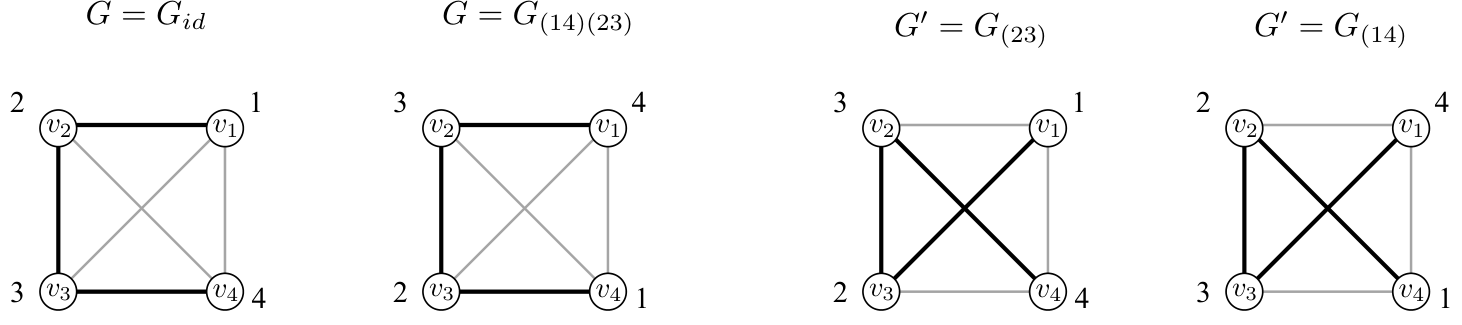
The key point of using labels on the vertices is to keep track of the role each vertex and each edge is playing in each of the copies of $G$. More precisely, note that the corresponding copies of the vertices and edges of $G$ in $G_{\sigma}$ are given by their labels: The copy of vertex $v_{i}$ of $G$ is the vertex of $G_{\sigma}$ having label $i$, while the copy of an edge $v_{i}v_{j}\in E(G)$ is the edge of $G_{\sigma}$ having label $ij$. It is important to note that $L_{G_{\sigma}}=L_{G}$ for all $\sigma\in S_{X}$, i.e. the set of labels of the edges of $G$ remains invariant among all copies $G_{\sigma}$, $\sigma\in S_{X}$. Given the prescribed labeling, we can talk now about edge-replacements by means of elements in $L_{G}$. In this context, we will denote by $rs\to kl$ the edge-replacement that corresponds to deleting the edge with label $rs$ and adding the edge with label $kl$. When the edge-replacement $rs\to kl$ is feasible, it means that $G-v_{r}v_{s}+v_{k}v_{l}\cong G$. We denote with $\emptyset\to\emptyset$ the neutral edge-replacement, where no edge is replaced at all. We define now

as the set of all feasible edge-replacements of $G$ given by their labels together with the neutral edge-replacement. Let $R_{G}^{*}=R_{G}\setminus\{\emptyset\to\emptyset\}$. We will use sometimes the notation $e\to e^{\prime}\in R_{G}$ when we do not require to specify the labels of the vertices involved in the edge-replacement, and it includes the possibility that $e\to e^{\prime}$ is the neutral edge-replacement.

Notice that, since feasible edge-replacements are defined by the labels of the edges, any $e\to e^{\prime}\in R_{G}$ represents also a feasible edge-replacement of any copy $G_{\sigma}$, $\sigma\in S_{X}$. Hence, clearly $R_{G_{\sigma}}=R_{G}$ for any $\sigma\in S_{X}$.

Given a feasible edge-replacement $rs\to kl\in R_{G}^{*}$ we will use the following notation

and we will set ${\rm Fer}_{G}(\emptyset\to\emptyset)=A_{G}$.

That is, ${\rm Fer}_{G}(e\to e^{\prime})$ is the set of permutations representing the $|{\rm Aut}(G)|$ different copies of $G$ that one can get to by means of performing the feasible edge-replacement $e\to e^{\prime}\in R_{G}$.

Observe that performing a feasible edge-replacement $e\to e^{\prime}\in R_{G}$ in a copy $G_{\rho}$ of $G$ yields the copy of $G$ given by the permutation $\sigma\,\rho$, where we can choose any $\sigma\in{\rm Fer}_{G}(e\to e^{\prime})$. In other words, we can model the application of a series of feasible edge-replacements by considering the composition of the corresponding permutations. A formal proof of this rather intuitive fact can be found in Lemma 8.1 in the Appendix. It now makes sense to consider the group ${\rm Fer}(G)$ generated by the permutations associated to all feasible edge-replacements, that is, by the set

Thus,

Clearly, ${\rm Fer}(G)$ acts on the set $\{G_{\sigma}\;|\;\sigma\in S_{X}\}$ by means of $(\rho,G_{\sigma})\mapsto G_{\rho\sigma}$, where $\rho\in{\rm Fer}(G)$ and $\sigma\in S_{X}$. Observe that this action represents what happens when a series of feasible edge-replacements, represented by $\rho$, is performed on a copy $G_{\sigma}$ of $G$: the result is the graph $G_{\rho\sigma}$. Hence, the property of being able to go from any copy $G_{\sigma}$ to any other $G_{\sigma^{\prime}}$ by means of a chain of feasible edge replacements means that, for any $\sigma,\sigma^{\prime}\in S_{X}$, there is a $\rho\in{\rm Fer}(G)$ such that $\sigma^{\prime}=\rho\sigma$, i.e. ${\rm Fer}(G)=S_{X}$. Recall also that, by Proposition 2.6, if $G\cup t_{0}K_{1}$ is a local amoeba for some $t_{0}>0$, then actually $G\cup tK_{1}$ is a local amoeba for every $t\geq t_{0}$. Thus, we can define now local and global amoebas by means of the group ${\rm Fer}(G)$.

We shall also note that ${\rm Aut}(G)\cong A_{G}=\{\sigma\in S_{X}\,|\,G_{\sigma}=G\}\leq{\rm Fer}(G)$. In the next lemma, we discuss the connection between the feasible edge-replacements of a graph $G$ and those of its complementary graph $\overline{G}$, concluding that the corresponding associated groups are the same.

As a consequence, we note the following.

To continue, we need some terminology. Given a subgroup $\Gamma\leq S_{X}$ and $k\in X$, we denote by $\Gamma k$ the orbit of $k$ by means of the canonical action of $\Gamma$ on $X$, i.e.

If, for some $Y\subseteq X$ and some $k\in Y$, we have that $\Gamma k=Y$, then we say that $\Gamma$ acts transitively on $Y$. We denote by ${\rm Stab}_{\Gamma}(Y)$, the stabilizer of $\Gamma$ on $Y$, that is

For an $x\in X$, we write ${\rm Stab}_{\Gamma}(x)$ instead of ${\rm Stab}_{\Gamma}(\{x\})$. Moreover, for $\sigma\in S_{X}$ and $Y\subseteq X$, we denote with $\sigma\raise-2.15277pt\hbox{$|$}_{Y}$ the restriction of $\sigma$ to $Y$, i.e. the mapping $\sigma\raise-2.15277pt\hbox{$|$}_{Y}:Y\to X$ defined by $\sigma\raise-2.15277pt\hbox{$|$}_{Y}(y)=\sigma(y)$ for $y\in Y$. Given sets $A,B,X,Y$ and two mappings $\sigma:A\to X$, and $\tau:B\to Y$ such that $\sigma(i)=\tau(i)$ for every $i\in A\cap B$, we denote with $\sigma\cup\tau$ the union of $\sigma$ and $\tau$, that is, the function $\sigma\cup\tau:A\cup B\to X\cup Y$ such that

According to Definition 3.2, in order to determine whether a graph $G$ with a vertex labeling $\lambda:V(G)\to X$ is a local amoeba, we need to demonstrate that ${\rm Fer}(G)=S_{X}$. Therefore, any way that enables us to generate the symmetric group $S_{X}$ using a small number of specific permutations would be advantageous. For example, the following are well known facts:

• •

  For any $i\in[1,n]$ we have that $S_{n}=\left\langle(1\;2\;3\ldots\;n),(i\;i+1)\right\rangle$.

• •

  The set $\{(i\;n)\;|\;i\in[n-1]\}$ generates $S_{n}$.

• •

  Let $X$ be a finite set, and let $k\in X$. Then, for any subgroup $\Gamma\leq{\rm Stab}_{S_{X}}(k)$ which is transitive on $X\setminus\{k\}$, we have that $S_{X}=\langle\Gamma\cup\{(i\;k)\}\rangle$, where $i$ is any element of $\in X\setminus\{k\}$.

Due to this, we can derive the following observation.

Next, we will show how Definition 3.2 is very handy by completing the proof of items (iii) and (iv) of Example 2.5. We also present an example that will be used in Section 5. The different feasible edge-replacements performed in Example 3.6 together with the corresponding permutations are illustrated Figure 3.

The graphs $P_{n}$, $\frac{n}{2}K_{2}$ and $C(n,1)$ are still quite basic examples to test to which amoeba family they belong. However, a simple application of the definition is not that easy to use when we consider a little more complicated graphs (not necessarily large ones). For example, the graph depicted below in Figure 4 can be shown to be a global amoeba and that it is not a local amoeba. We will prove this later on by means of more sophisticated tools that we will develop (see Example 4.3). Meanwhile, we leave to the reader to play around with this example.

We will finish this section with an interesting example that will play an important role in Section 6. Let $H_{n}$ be the graph of order $n\geq 2$ with $V(H_{n})=A\cup B$ such that, taking $q=\lfloor\frac{n}{2}\rfloor$, $A=\{v_{1},v_{2},\ldots,v_{q}\}$ and $B=\{v_{q+1},v_{q+2},\ldots,v_{q+{\lceil\frac{n}{2}\rceil}}\}$, where $B$ is a clique, $A$ is an independent set and adjacencies between $A$ and $B$ are given by $v_{i}v_{q+j}\in E(H_{n})$ if and only if $j\leq i$, where $1\leq i\leq q$ and $1\leq j\leq\lceil\frac{n}{2}\rceil$ (see Figure 5). Observe that $\deg(v_{i})=i$ for all $1\leq i\leq q$ and $\deg(v_{q+j})=n-j$ for all $1\leq j\leq\lceil\frac{n}{2}\rceil$. Hence, we have one vertex from each degree between $1$ and $n-1$ with exception of vertices $v_{q}$ and $v_{n}$ that have both degree $\lfloor\frac{n}{2}\rfloor$.

References

- [1] N. Alon, Y. Caro, I. Krasikov, Y. Roditty, Combinatorial reconstruction problems, J. Combin Theory Ser. B 47 (1989), no. 2, 153 – 161.
- [2] L. Babai, Graph Isomorphism in Quasipolynomial Time. arXiv preprint, arXiv:1512.03547.
- [3] L. Babai, http://people.cs.uchicago.edu/ laci/update.html
- [4] L. Babai, E. M. Luks. Canonical labeling of graphs. Proceedings of the Fifteenth Annual ACM Symposium on Theory of Computing (1983), 171–183.
- [5] Y. Bagheri, A. R. Moghaddamfar, F. Ramezani. The number of switching isomorphism classes of signed graphs associated with particular graphs, Discrete Appl. Math. 279 (2020), 25–33.
- [6] S. Bau, B. van Niekerk, D. White. An intermediate value theorem for the decycling numbers of Toeplitz graphs, Graphs Combin. 31 (2015), no. 6, 2037–2042.
- [7] M. Behzad, G. Chartrand, No graph is perfect, Amer. Math. Monthly 74 (1967), 962–963.
- [8] J. A. Bondy. Bounds for the Chromatic Number of a Graph, J. Combinatorial Theory 7(1969), 96–98.
- [9] G. Călinescu, A. Dumitrescu, J. Pach, Reconfigurations in graphs and grids, SIAM J. Discrete Math. 22 (2008), no. 1, 124–138.
- [10] Y. Caro, A. Hansberg, A. Montejano. Recursive constructions of amoebas, Procedia Computer Science, Volume 195 (2021) 257-265.
- [11] Y. Caro, A. Hansberg, J. Lauri, C. Zarb. On zero-sum spanning trees and zero-sum connectivity. Electron. J. Combin. 29 (2022), no. 1, Paper No. 1.9.
- [12] Y. Caro, A. Hansberg, A. Montejano. Unavoidable chromatic patterns in 2-colorings of the complete graph. J. Graph Theory 97 (2021), no. 1, 123–147.
- [13] S. Cichacz, I. A. Zioło. -swappable graphs, AKCE Int. J. Graphs Comb. 15 (2018), no. 3, 242–250.
- [14] D. Conlon, J. Fox, Bounds for graph regularity and removal lemmas, Geometric and Functional Analysis 22 (2012), no. 5, 1191–1256,
- [15] P. Czimmermann, Representation of the reconstruction conjecture by group actions, Journal of Information, Control and Management Systems 3 (2005), No. 2, 75 – 80.
- [16] P. Erdős, Some combinatorial, geometric and set theoretic problems in measure theory, in Kölzow, D. Maharam-Stone, D. (eds.), Measure Theory Oberwolfach 1983, Lecture Notes in Mathematics (1984), vol. 1089, Springer.
- [17] R. Fabila-Monroy, D. Flores-Peñaloza, C. Huemer, F. Hurtado, J. Urrutia, D.R. Wood, Token graphs, Gr. Combin. 28(3) (2012), 365–380.
- [18] J. Fresán-Figueroa, E. Rivera-Campo. On the fixed degree tree graph, J. Inform. Process. (2017) 25, 616–620.
- [19] D. Froncek, A. Hlavacek, S. Rosenberg. Edge reconstruction and the swapping number of a graph, Australas. J. Combin. 58 (2014), 1–15.
- [20] J. R. González-Martínez, M. E. Gonzalez-Laffitte, A. Montejano. Computational detection of the amoeba graph family and the case of weird edge-replacements (preprint).
- [21] Gonález-Laffite, Marcos, https://github.com/MarcosLaffitte/Amoebas
- [22] F. Harary, R. Mokken, M. Plantholt. Interpolation theorem for diameters of spanning trees, IEEE Trans. Circuits and Systems 30 (1983), no. 7, 429–432.
- [23] F. Harary, M. J. Plantholt, Classification of interpolation theorems for spanning trees and other families of spanning subgraphs, J. Graph Theory. 13 (1989), no.6, 703–712.
- [24] S. G. Hartke, H. Kolb, J. Nishikawa, D. Stolee, Automorphism group of a graph and a vertex-deleted subgraph, Electron. J. Combin. 17 (2010), no. 1, Research paper 134, 8 pp.
- [25] D. Horsley. Switching techniques for edge decompositions of graphs, Surveys in combinatorics 2017, 238–271, London Math. Soc. Lecture Note Ser., 440, Cambridge Univ. Press, Cambridge, 2017.
- [26] I.M. Isaacs, Finite Group Theory, in: Graduate Studies in Mathematics, vol. 92, American Mathematical Society, Providence, RI (2008).
- [27] T. Ito, E. D. Demaine, N. J. A. Harvey, C. H. Papadimitriou, M. Sideri, R. Uehara, Y. Uno, On the complexity of reconfiguration problems, Theoret. Comput. Sci. 412 (2011), no. 12–14, 1054–1065.
- [28] D. A. Jaume, A. Pastine, V. N. Schvöllner. 2-switch: transition and stability on graphs and forests, arXiv preprint, arXiv:2004.11164 , 2020.
- [29] P. Kaski, P. R. J. Östergård. Classification algorithms for codes and designs. Algorithms and Computation in Mathematics, 15. Springer-Verlag, Berlin, 2006.
- [30] J. Lauri, R. Scapellato. Topics in graph automorphisms and reconstruction. Second edition. London Mathematical Society Lecture Note Series, 432 (2016), xiv+192 pp.
- [31] J. Leaños, A. L. Trujillo-Negrete, The connectivity of token graphs. Graphs Combin. 34 (2018), no. 4, 777–790.
- [32] K. Lih, C. Lin, L. Tong. On an interpolation property of outerplanar graphs, Discrete Appl. Math. 154 (2006), no. 1, 166–172.
- [33] B. D. McKay, Practical graph isomorphism. Congr. Numer. 30 (1981), 45–87.
- [34] B. D. McKay, A. Piperno. Practical graph isomorphism, II. J. Symbolic Comput. 60 (2014), 94–112.
- [35] E. Melville, B. Novick, S. Poznanović, On reconfiguration graphs: an abstraction, Australas. J. Combin. 81 (2021), 339–356.
- [36] N. Punnim. Interpolation theorems on graph parameters, Southeast Asian Bull. Math. 28 (2004), no. 3, 533–538.
- [37] N. Punnim. Switchings, realizations, and interpolation theorems for graph parameters, Int. J. Math. Math. Sci. 2005, no. 13, 2095–2117.
- [38] A. J. Radcliffe, A. D. Scott, Reconstructing under group actions, Graphs Combin. 22 (2006), 399 – 419.
- [39] M. S. Ross. 2-swappability and the edge-reconstruction number of regular graphs, arXiv preprint, arXiv:1503.01048, 2015.
- [40] T. Seppelt, The Graph Isomorphism Problem: Local Certificates for Giant Action, arXiv:1909.10260.
- [41] A. Seress, Permutation group algorithms, Cambridge University Press, 2003.
- [42] D. J. A. Welsh, M. B. Powell, An Upper Bound for the Chromatic Number of a Graph and Its Application to Timetabling Problems, Comput. J. 10 (1967), 85–86.
- [43] D. B. West. Introduction to graph theory. Prentice Hall, Inc., Upper Saddle River, NJ (1996), xvi+512 pp.
- [44] S. Zhou. Interpolation theorems for graphs, hypergraphs and matroids, Discrete Math. 185 (1998), no. 1-3, 221–229.