Hydrodynamic Simulations of Pre-Supernova Outbursts in Red Supergiants: Asphericity and Mass Loss
Abstract
The activity of massive stars approaching core-collapse can strongly affect the appearance of the star and its subsequent supernova. Late-phase convective nuclear burning generates waves that propagate toward the stellar surface, heating the envelope and potentially triggering mass loss. In this work, we improve on previous one-dimensional models by performing two-dimensional simulations of the pre-supernova mass ejection phase due wave heat deposition. Beginning with stellar evolutionary models of a 15 red supergiant star during core O-burning, we treat the energy deposition rate and duration as model parameters and examine the mass-loss dependence and the pre-explosion morphology accordingly. Unlike one-dimensional models, density inversions due to wave heating are smoothed by Rayleigh-Taylor instabilities, and the primary effect of wave heating is to radially expand the star’s hydrogen envelope. For low heating rates with long durations, the expansion is nearly homologous, whereas high but short-lived heating can generate a shock that drives envelope expansion and results in a qualitatively different density profile at the time of core-collapse. Asymmetries are fairly small, and large amounts of mass loss are unlikely unless the wave heating exceeds expectations. We discuss implications for pre-supernova stellar variability and supernovae light curves.
pacs
26.30.-k,keywords
(stars:) stellar evolution – hydrodynamics – atmosphere1 Introduction
1.1 Pre-Supernova Stellar Evolution
Type II supernovae (SNe) are the explosions of massive hydrogen-rich stars, and it is widely accepted that the progenitors of type II-P SNe are red supergiants. Observations indicate that progenitor stars of interacting Type IIn SNe usually produce pre-SN outbursts (Ofek et al. 2014), specific examples including SN 2009ip (Mauerhan et al. 2013), SN 2010mc (Ofek et al. 2013) and SN 2015bh (Elias-Rosa et al. 2016; Ofek et al. 2016). However, even fairly typical type IIP SNe show evidence for circumstellar material (CSM) that may arise from pre-SN mass loss (Khazov et al. 2016; Yaron et al. 2017). Pre-SN mass eruption events have also been observed or hinted in other types of SNe, including Type IIb such as SN 2013cu (Gal-Yam et al. 2014; Groh 2014; Gräfener & Vink 2016), Type Ibn such as SN 2006jc (Pastorello et al. 2007), SN 2015G (Shivvers et al. 2017), SN 2015U (Shivvers et al. 2016), and even broad-lined Type Ic such as PTF11qcj (Corsi et al. 2014) and 2018gep (Ho et al. 2019).
Pre-SN mass ejection has been proposed to explain many features of both ordinary and super-luminous SNe. The interaction between the ejecta from the final core-collapse explosion and the previously ejected circumstellar material allows the efficient conversion of the ejecta kinetic energy to thermal energy by shock heating. A classical example is pulsation pair-instability SNe (Woosley et al. 2007; Yoshida et al. 2016; Woosley 2018; Leung et al. 2019a). Shock waves driven by unstable oxygen burning eject large amounts of mass prior to the star’s collapse, creating dense CSM that allows for a super-luminous SN (Sorokina et al. 2016; Morozova et al. 2017; Tolstov et al. 2017).
For less massive stars, wave energy transport within the progenitor may be able to trigger smaller amounts of pre-SN mass loss (Quataert & Shiode 2012, see e.g.). Due to the large energy generation rate by nuclear reactions, convective motions near the star’s core become very energetic during advanced burning phases such as carbon, neon, oxygen, and silicon burning (Woosley et al. 2002, e.g.). The convective motion generates gravity waves that carry a power that scales with the convective luminosity as (Goldreich & Kumar 1990; Alvan et al. 2015), where is the mean Mach number of the convective motion. The gravity waves propagate outwards and are partially reflected by overlying convective shells, though some wave energy is still transferred outwards into acoustic waves after tunneling through these evanescent regions (see, e.g., Fuller et al. 2015; Takata 2016 for applications in low-mass red-giant stars).
The acoustic waves dissipate via weak shock formation when the energy transport rate by wave exceeds the maximum possible wave flux (Ro & Matzner 2017), which drops rapidly at the transition from the helium shell to the hydrogen envelope. The thermalized wave energy, depending on how fast it is injected, can trigger expansion of the envelope and also mass ejection (Fuller 2017). Recent studies of observational data have shown that pre-SN activity may be important for explaining the light curve shape (Moriya et al. 2017; Morozova et al. 2017; Moriya et al. 2018; Morozova et al. 2018), though too much wave heat (or heat deposited over too long of a duration) is inconsistent with typical type II-P SNe (Ouchi & Maeda 2019). Instead, more impulsive wave heating is favored based on light curve modeling of SN 2017eaw, confirming that such energy deposition can better reproduce SN light curves (Morozova et al. 2020).
We note that wave-driven outbursts may not occur in many SN progenitors, as demonstrated by SN progenitor monitoring (Kochanek et al. 2017; Johnson et al. 2018) that rules out luminous and long-lasting outbursts in several nearby type II-P SNe. The purpose of this paper is not to determine the frequency or likelihood of wave-driven outbursts, but rather their effect on the progenitor’s structure if they do occur.
1.2 Motivation
Fuller 2017 and Fuller & Ro 2018 compute one-dimensional stellar evolutionary models for a star model with and without a hydrogen envelope. They demonstrate that wave heat has very different effects in hydrogen-rich and hydrogen-poor stars. In the latter, the energy can eject in an optically thick super-Eddington wind from the surface of the star. In hydrogen-rich stars, however, wave energy is thermalized at the base of the hydrogen rich envelope and is likely insufficient to unbind the entire envelope. While small amounts of material may be unbound by a weak shock excited by wave heating, the one-dimensional models exhibit an inflation of the envelope as the extra thermal pressure blows a low-density “bubble” at the base of the hydrogen envelope.
However, the energy deposition can give rise to non-radial hydrodynamical instabilities that cannot be captured in any of the previous one-dimensional simulations. As mentioned above, wave energy deposition in a low-density bubble causes it to have a high thermal pressure but a low density. As it expands into the low-pressure and high-density envelope, Rayleigh-Taylor instability will occur at the interface between the bubble and the overlying envelope, strongly modifying the subsequent dynamics of the envelope’s response. It therefore becomes interesting to examine multi-dimensional simulations of the star’s response, which have never been performed in a systematic way for this process. In this work, we explore the general behaviour of the envelope in response to such energy deposition and examine the aspherical effects on the pre-SN mass loss and the envelope structure.
The organization of the paper is as follows. In Section 2, we describe the hydrodynamical formalism for modeling the wave energy deposition in the stellar envelope and how we construct the initial model. Then in Section 3 we present a benchmark model which demonstrates the typical effects of wave heating in multiple dimensions. In Section 4, we examine how the mass loss process and the envelope structure changes with the energy deposition and its duration. In Section 5, we discuss implications for supernovae and progenitor stars with different wave heating rates and durations. In the Appendix, we further show how our simulations depend some of the input parameters, including the mesh resolution, the initial perturbation and the boundaries.
2 Methods
2.1 Stellar Model


To construct the initial models for the hydrodynamics run, we first use the one-dimensional stellar evolutionary code MESA (Modules for the Experiments in Stellar Astrophysics, Paxton et al. 2011; Paxton et al. 2013; Paxton et al. 2015; Paxton et al. 2017; Paxton et al. 2019) version 8118. We evolve a 15 star with solar metallicity, starting at the a zero-age main-sequence. The simulation continues until the central density approaches g cm-3. Then we extract the stellar profile when the star is carrying out core O-burning and map the stellar profile to our two-dimensional mesh.
In the top left panel of Figure 1 we plot a Hertzsrung-Russell diagram of the model’s evolution, and in the top right panel of Figure 1 we plot the time evolution of the nuclear, neutrino and surface luminosities of the stellar model. The surface luminosity does not vary during the late-stage vigorous nuclear burning in the core, but the neutrino luminosity in general follows the nuclear luminosity. Note that the shell burning of C and Ne triggers a brief jump in the nuclear luminosity, while O-burning provides a more steady energy production. In the bottom right panel of Figure 1, we plot the density and temperature profile of the MESA profile. We model only the outer part beyond in the simulations, corresponding to at the base of the H-envelope where the wave heating is expected to take place.
2.2 Hydrodynamics
We use a two-dimensional hydrodynamics code which we previously used extensively for SN simulations. The code is designed for multiple purposes and has been used in simulations of Type Ia SNe (Leung et al. 2015; Leung & Nomoto 2018; Leung & Nomoto 2020), electron capture SNe (Leung & Nomoto 2017; Leung & Nomoto 2019; Leung et al. 2020; Zha et al. 2019b) and accretion-induced collapse (Leung et al. 2019b; Zha et al. 2019a). The code utilizes the fifth-order shock capturing WENO (Barth & Deconinck 1999) and the five-step third-order non-strong-stability preserving Runge-Kutta scheme for time-discretization (Wang & Spiteri 2007) of the Euler equations. In this work, we consider the equatorial plane of the star in polar coordinates (). This allows the use of a reflective boundary in the radial direction and a periodic boundary in the -direction. To perform the simulations in a computationally feasible time range, we run the simulations in a single quadrant.
To close the equations, we use the Helmholtz equation of state (Timmes et al. 2000). This equation of states consists of contributions from electron gas with arbitrary degeneracy, ions in the form of an ideal gas, photons in the Planck distribution, and electron-positron pairs. We use a reflective boundary for the radial inner boundary, and a free-flow boundary for the radial outer boundary. When the energy deposition is strong, the fluid near the inner boundary can expand significantly, causing mass flow outwards. In that case, we provide additional mass to the innermost grid cells such that the outflow mass is balanced by the additional mass, as it would be in a real star by upwelling material. Then, we inject the corresponding gravitational energy to the system to maintain energy conservation and adjust the mass cut value. This ensures that the total mass and energy, including both the hydrodynamical grids and the mass-cut, are conserved as a whole.
2.3 Energy Deposition
Below we describe the changes to the code in order to accommodate the wave heating physics. We consider a wave luminosity emerging from the core, , which propagates into our computational domain and then dissipates into heat. We model only the heat dissipation and not the waves themselves. In each time step, we compute how much energy is deposited in each of the computational mesh points by comparing the maximal luminosity and the local which decreases with radius as wave energy is converted into heat. When , no change in is made. Otherwise, the new is computed by solving (see e.g., Landau & Lifshitz 1959; Ulmschneider 1970; Mihalas & Mihalas 1984; Fuller & Ro 2018 for derivations)
| (1) |
This formula is appropriate for waves that gradually steepen to form weak shocks (i.e., the post shock pressure only slightly exceeds the pre-shock pressure), which occurs when is slightly larger than . As discussed in Fuller & Ro 2018, the weak shock damping prevents the waves from steepening into strong shocks with , so the approximation of equation 1 is good throughout most of the wave energy deposition region.
The relative change can be very steep for a high value of . We smooth by hand the energy deposition to a mass with a minimum of , which ensures the process of energy deposition is resolved at the current resolution. To do this, the energy along each ray with a given is smoothed over a mass , where is the number of grid points along the -direction. In each step, we search along a constant -direction for the transition position () where . Then we integrate outward to look for the outer radius so that the accumulated mass . The local energy deposition in each grid cell is the mass of the cell divided by .
2.4 Initializing Hydrodynamics
After evolving the stellar model, we take one snapshot during core O-burning, and map the density and pressure into our 2D simulation. The profile from the stellar evolution code obeys hydrostatic equilibrium. However, during mapping from the Lagrangian MESA mesh to the Eulerian simulation mesh, slight departures from hydrostatic equilibrium can be introduced. For the inner boundary, we chose a mass cut of mass with a radius cm, near the base of the hydrogen envelope and below the initial wave heating region. We use a uniform 1500x30 grid with a radial grid size cm and angular grid size of 3 .
In Appendix A, we further study how our model achieves hydrostatic equilibrium after it is mapped to our hydrodynamics model. While radial motion and changes to the density profile do occur, they are smaller than those caused by the wave heating which we examine below. Additionally, convection is not present in the initial model, which may underestimate the energy transport at early times if convective flows can help channel the deposited energy away.
The initial profile is spherically symmetric, so we add density perturbations in the form . We choose in this work. In Appendix C we demonstrate that the exact value of does not change our results. The density perturbation is added to mimic the inherent density fluctuations due to convection, and aims at seeding the growth of non-radial instabilities. The value is chosen such that the total mass is conserved globally and along each radial direction. This prevents global motion of the star in any specific direction.

3 Benchmark Model
Here we focus on this benchmark model, and in Section 5 we further discuss the dynamics based on models of different progenitor masses.
3.1 Hydrodynamical Response of Benchmark model
When the energy deposition starts, the heated region is usually within a narrow band of radius near the bottom of the simulation domain. As outlined in the previous section, the deposition region is smoothed along 0.1 starting from the innermost grid point with energy deposition. For our benchmark model the heating rate is set to and lasts for 120 days. In Figure 2, we show density color plots of the benchmark model at different time slices to show how the star expands and contorts due to energy deposition. The energy deposition creates a layered structure, due to weak shocks propagating through the envelope, as seen in Day 114. Like the 1D models, the 2D models exhibit a “bubble” of lower density within the envelope, but with a weaker density inversion. At day 114, the bubble surface is near cm but expands outwards, and by day 228, the bubble surface is wavy due the density perturbations introduced in our initial conditions. The heating ceases after day 120, but the star does not expand significantly until after day 200 when the heat-induced pressure wave reaches the stellar surface. The core also develops non-radial structures due to non-radial instabilities and flows driven by the heating.
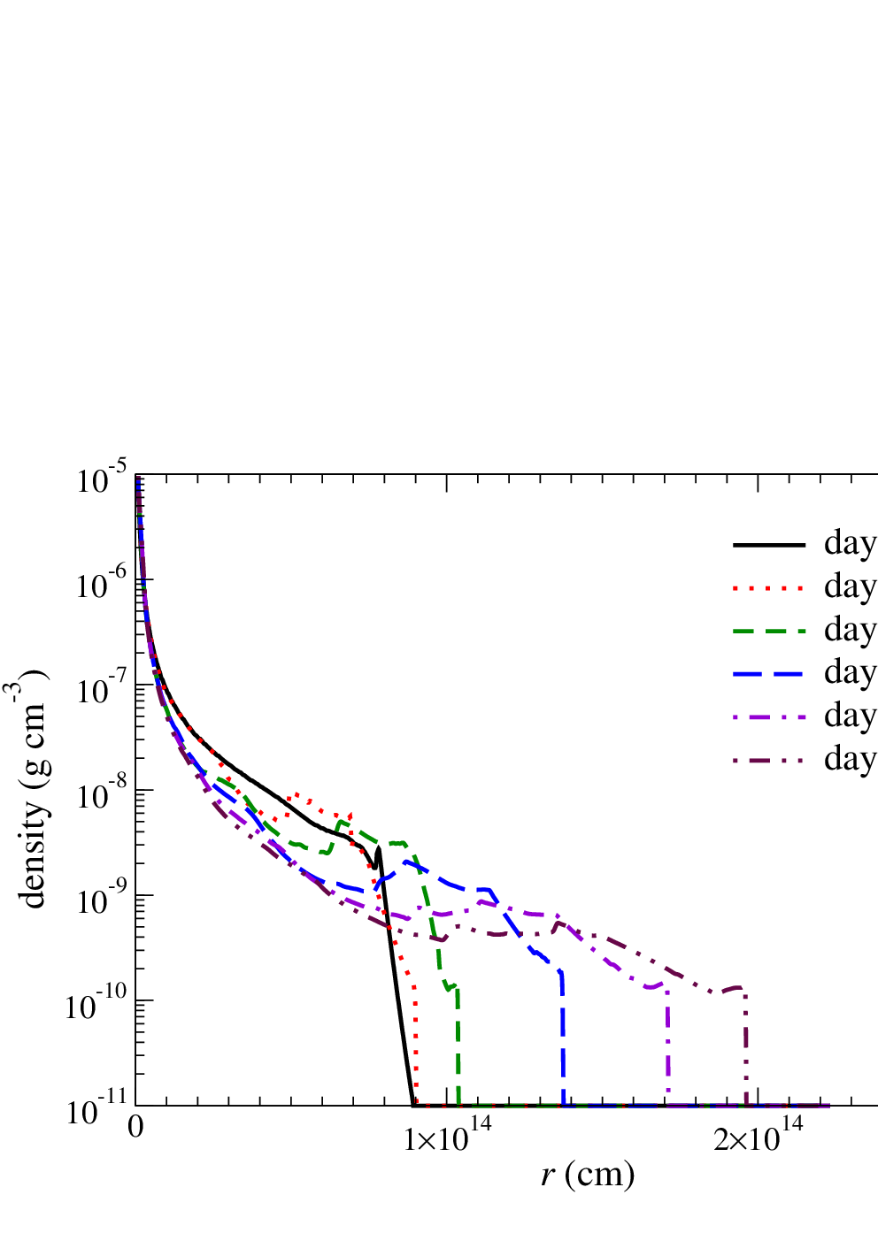
We plot in Figure 3 the angle-averaged density profiles of the benchmark model at selected times to further analyze the density and velocity evolution of the ejecta. The energy deposition takes place near the core at cm, driving a density inversion which propagates outward. The density difference can be a factor of 3 between the minimum value in the trough to the peak. The angle-averaged density inversion gradually smooths out as the star expands, due to the growth of the Rayleigh-Taylor instability from the seed perturbations added to the model, which create the wavy patterns seen in Figure 2.
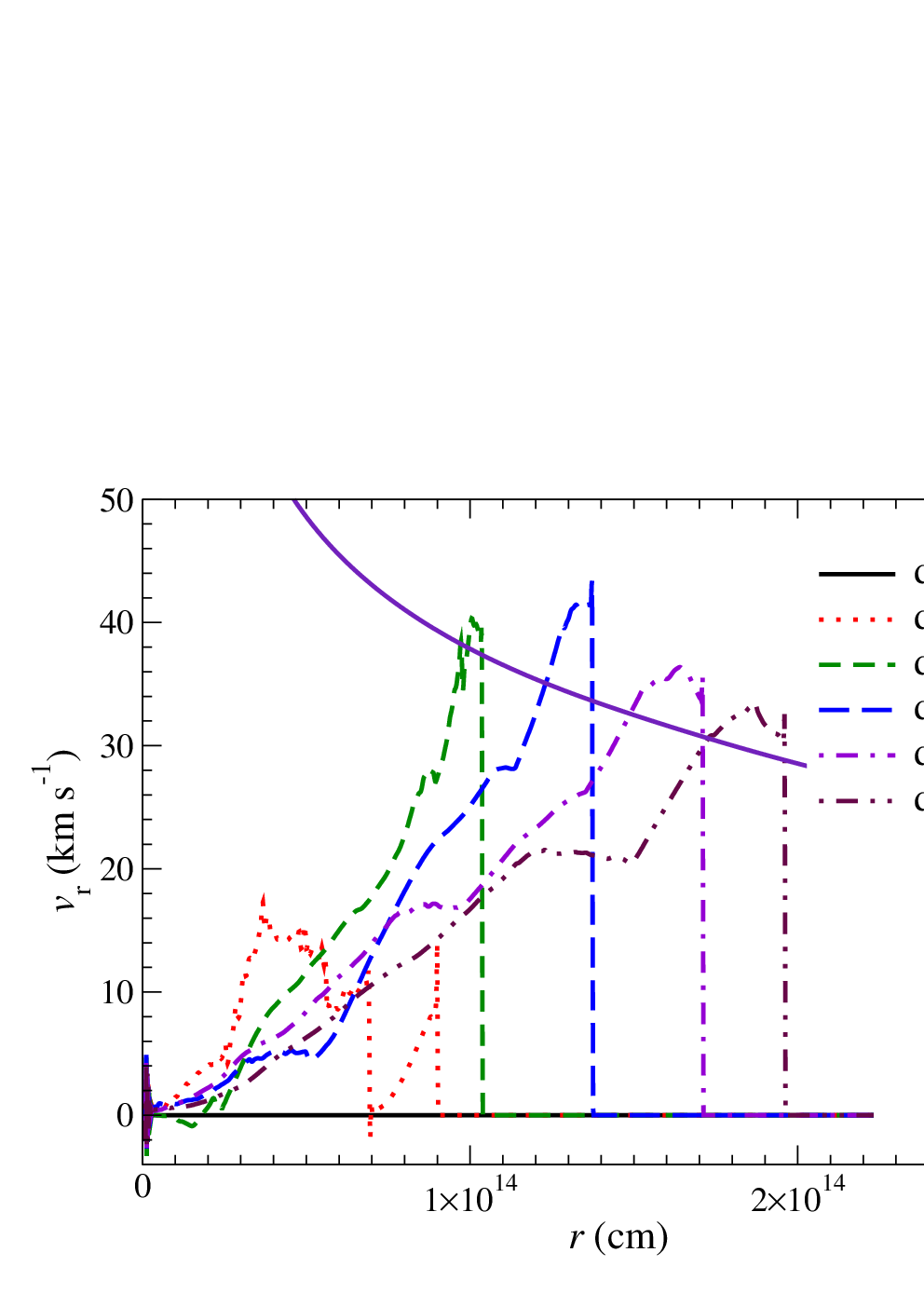
In the left panel of Figure 4, we plot the angle-averaged radial velocity profile of the benchmark model. The energy deposition occurring in the first 120 days drives expansion of the envelope, with internal velocities km s-1. When this velocity/pressure wave reaches the surface where the density is small, it steepens into a shock to trigger a rapid expansion of the envelope. The velocity can be as high as km s-1, near the escape speed of the star’s surface. As the envelope expands, it slows down due to gravity, approaching km s-1 at 570 days after the start of energy deposition.
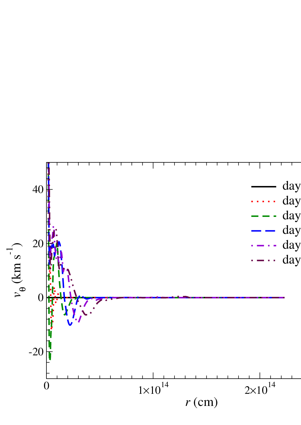
To further understand the asphericity of the ejecta, we also plot in the bottom panel of Figure 4 the angle-averaged angular velocity snapshots. Most of the star has a smaller angular velocity compared to the radial velocity, but the angular velocity reaches km s-1 within the innermost cm. The direction of the angular flow changes with both radius and time due to its turbulent nature. Beyond cm, there is no observable motion in the angular velocity.
In this model, there is no direct mass ejection. The outer boundary at cm is sufficiently large to contain all matter during the simulation. Only the outer layers of the star achieve velocities close to the escape velocity. While pressure gradients may still provide extra acceleration, the sub-escape velocities of inner layers suggests the net mass ejection will be low. Besides, after the O-burning has started, it takes year before the final collapse takes place, so there might not be sufficient time for any matter to escape before the final collapse.

Finally, we examine the energy budget of the benchmark model. In Figure 5, we plot the different components of energy as a function of time. The total energy grows linearly in the first 120 days due to the deposited energy in the model. Note also the small negative energy inflow due to the gravitational potential energy of mass added to the system as described in Section 2. Examining the gravitational energy and internal energy trends, we see that the star does not significantly expand in the first 100 days, but then expands noticeably, lowering the gravitational energy. The early growth and subsequent decline of internal energy shows that the system first stores the deposited energy in thermal energy, and later converts this into kinetic energy, which is then converted into gravitational energy as the star expands outward. We also note that the internal energy eventually decreases below its initial value, reflecting the nearly adiabatic losses during envelope expansion.
4 Dependence on Wave Heating Parameters
| Model | Duration | Unbound mass | remarks | ||||
| Unit | day | erg | erg | erg | |||
| 1 | 0.1 | 120 | 0.398 | -1.948 | -1.586 | 0.04 | |
| 2 | 0.1 | 360 | 1.195 | -1.948 | -1.033 | 1.3 | |
| 3 | 0.3 | 40 | 0.398 | -1.948 | -1.585 | 0.01 | |
| 4 | 0.3 | 120 | 1.195 | -1.948 | -1.055 | 0.26 | |
| 5 | 0.3 | 360 | 3.585 | -1.948 | 0.686 | 3.9 | |
| 6 | 1.0 | 40 | 1.195 | -1.948 | -1.153 | 0.18 | |
| 7 | 1.0 | 120 | 3.585 | -1.948 | 0.351 | 5.8 | |
| 4a | 0.3 | 120 | 1.195 | -1.948 | -1.049 | No | seed |
| 4b | 0.3 | 120 | 1.195 | -1.948 | -0.975 | No | seed |
| 4c | 0.3 | 120 | 1.195 | -1.948 | -1.053 | No | |
| 4d | 0.3 | 120 | 1.195 | -1.948 | -1.046 | No | |
| 4s | 0.3 | 120 | 1.195 | -1.948 | -0.685 | No | No initial seed |
In the previous section, we examined how the envelope responds to wave energy deposition for a benchmark model. Here, we extend our study to examine how these properties depend on the energy deposition rate and duration. Table 1 lists parameters of the models we have run, where the benchmark model is Model 4. We also remark that, another way to compare the model is by the total energy deposited. In this sense, Models 1 and 3 form the “low-energy model” (LEM); Models 2, 4 and 6 form the “medium-energy models” (MEM); and Models 5 and 7 form the “high-energy models” (HEM).
4.1 Dependence on Total Wave Heat
We first study how models with the same total deposited energy behave, from which we can extract some general observations about the effects of wave energy deposition.
4.1.1 Hydrodynamics of Low-Energy Models
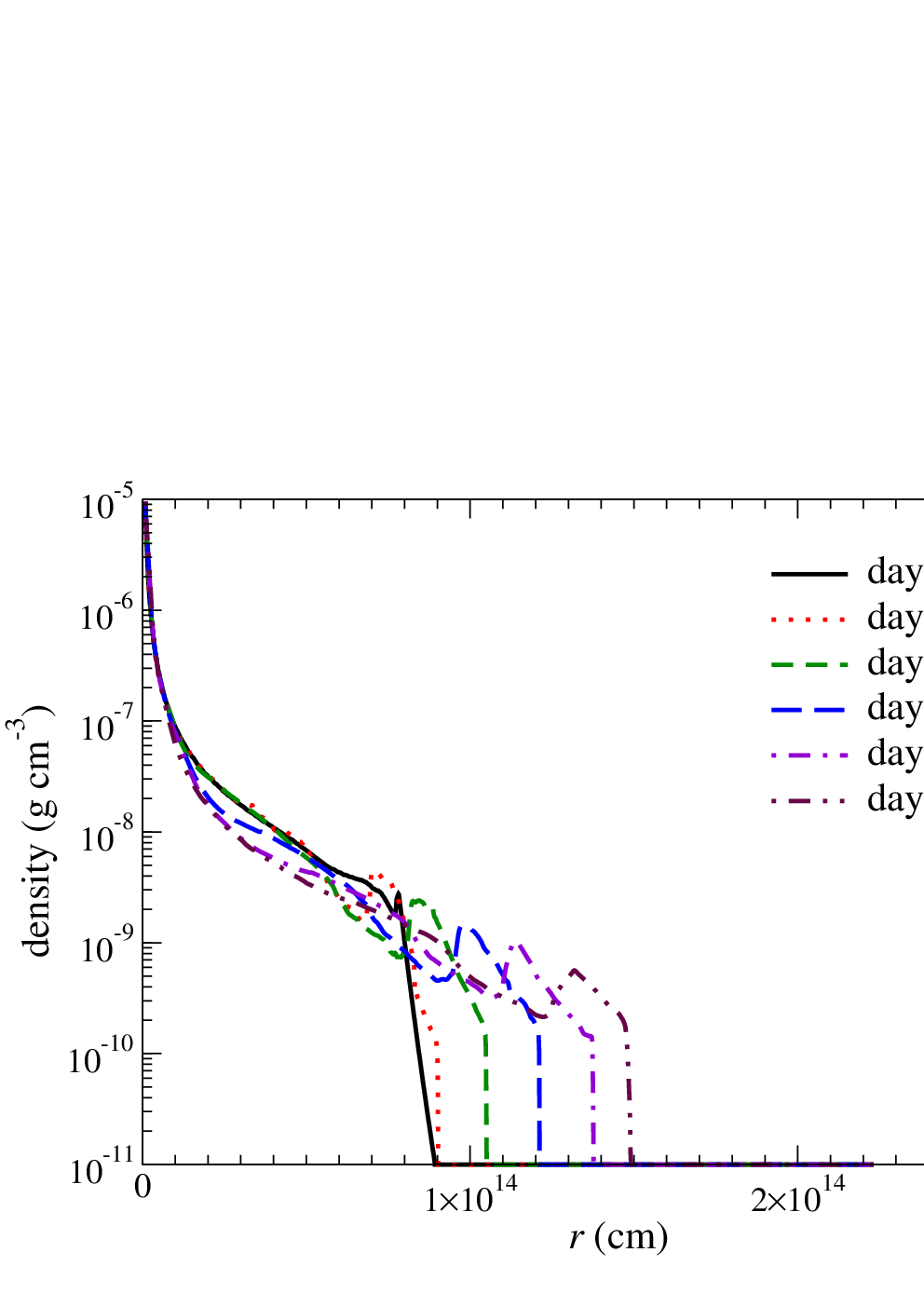
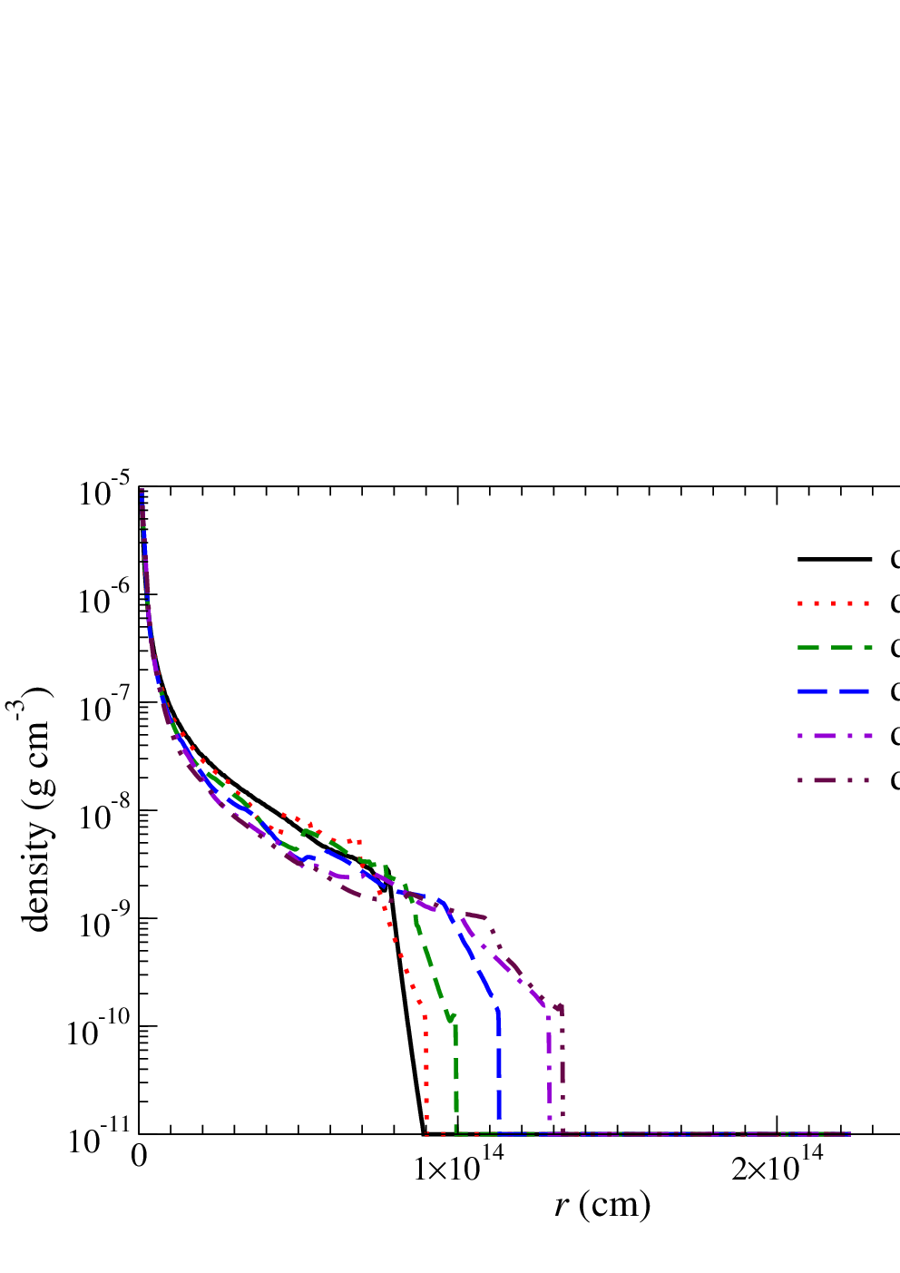
In Figure 6, we plot in the upper (lower) panel the density profiles of Model 1 (3) taken from the LEM. In Model 1, which has a lower , the star shows a regulated expansion. A density inversion (like that shown in the benchmark model) develops at cm at day 114 and slowly propagates to cm by day 570. The density contrast across the inversion nearly stays fixed at roughly a few times the minimum density, while the sharp density gradient at the surface remains. In Model 3, the expansion proceeds steadily without forming a density inversion. A strong shock does not form in either case, leaving a sharp density gradient at the surface, and all material in the star remains gravitationally bound.

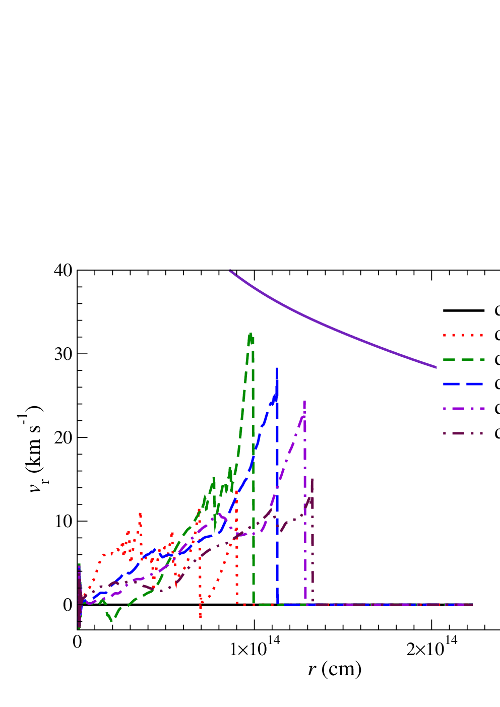
Figure 7 shows the radial velocity profiles of the LEM. In Model 1, the initial energy deposition triggers a pulse-like velocity profile at day 114 with a peak velocity of km s-1 at day 228. The whole star is gravitationally bound, including the shock-heated surface. Model 3 shows an erratic velocity profile characterized by shocks at early times, which can be seen at 3, 5, 7 and cm at day 114. After the shocks reach the surface, the star exhibits nearly “homologous” expansion in the sense that the expansion velocity is roughly proportional to radius. Again the velocity is too low to escape the star directly. The surface velocity is only 15 km s-1 at the end of the simulation.
These two models suggest that the actual changes in the density and velocity profiles are almost negligible in the low energy regime. The heat triggers moderate expansion but no major restructuring of the density profile.
4.1.2 Hydrodynamics of Medium-Energy Models
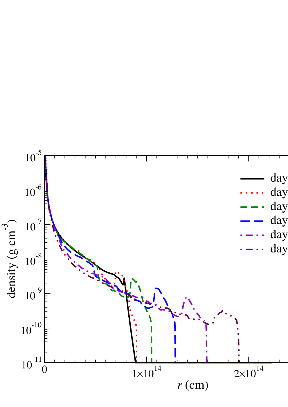
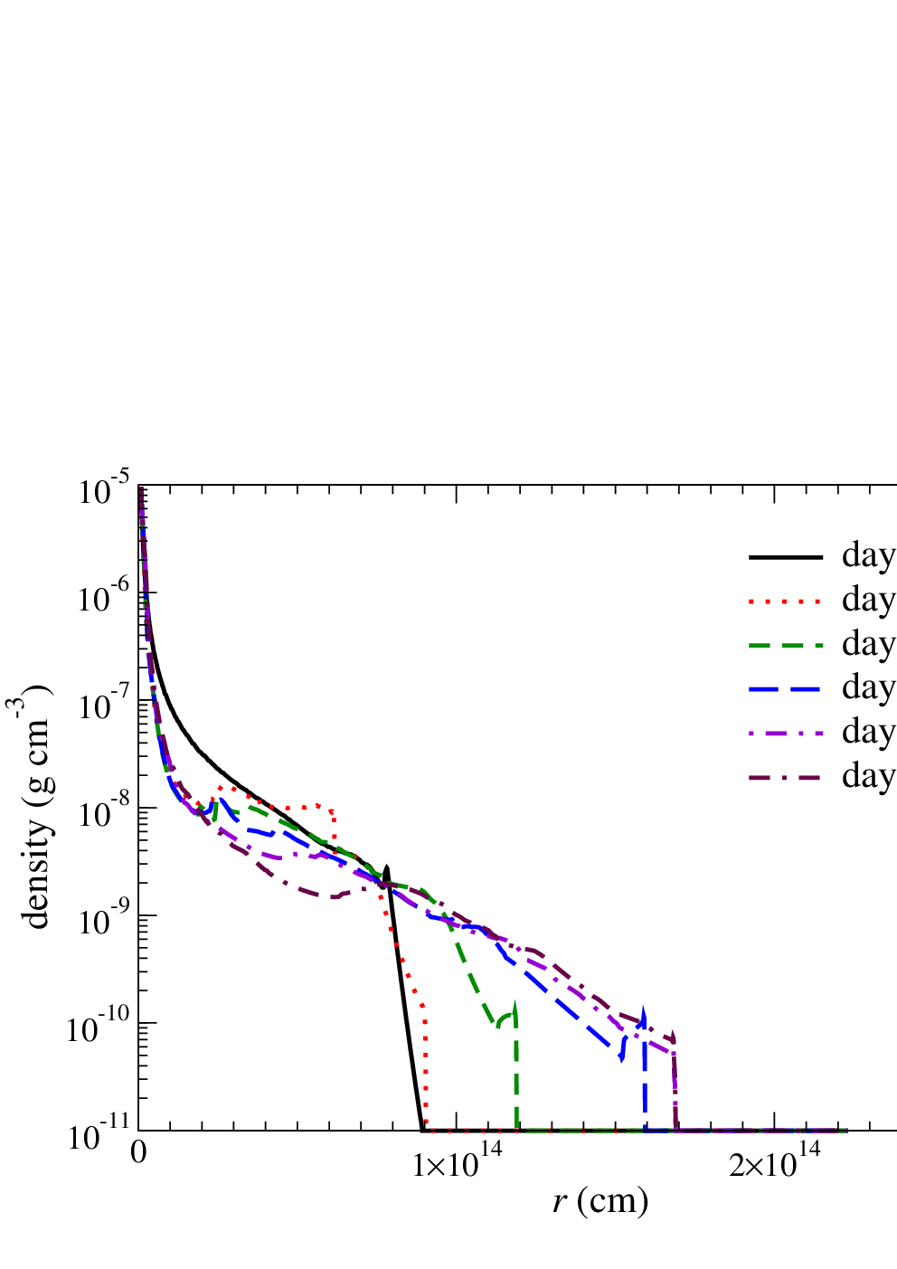
In Figure 8 we plot the density profiles of two models with the same energy input as the benchmark model, with erg, but at a low heating rate of for 360 days (Model 2) and at a high heating rate of for 40 days (Model 6). The lower energy deposition in Model 2 creates a density inversion which mildly accelerates with time as the density contrast approaches the surface. The density difference can be a few times higher than the minimum density at the trough. The star smoothly expands to cm. In Model 6, there is no significant density inversion developed in the whole simulation, except a small one near the surface. The stellar density profile is mostly monotonically decreasing and expanding, signifying a smooth expansion. The outer layers stagnate at the end of the simulation, suggesting that the star’s expansion slows down, with all of its matter remaining bound.
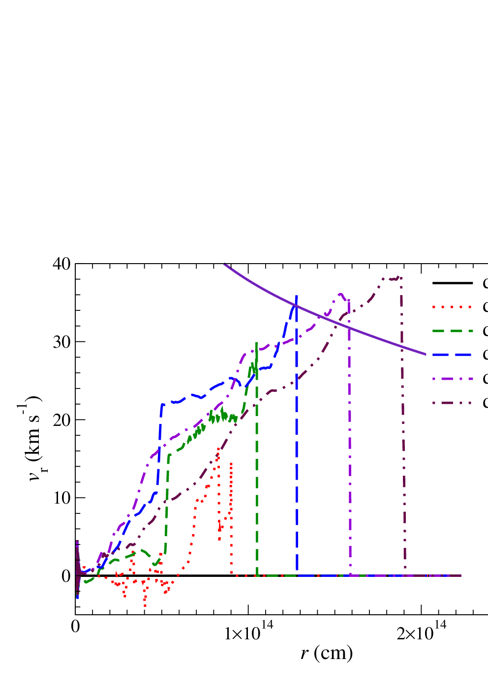
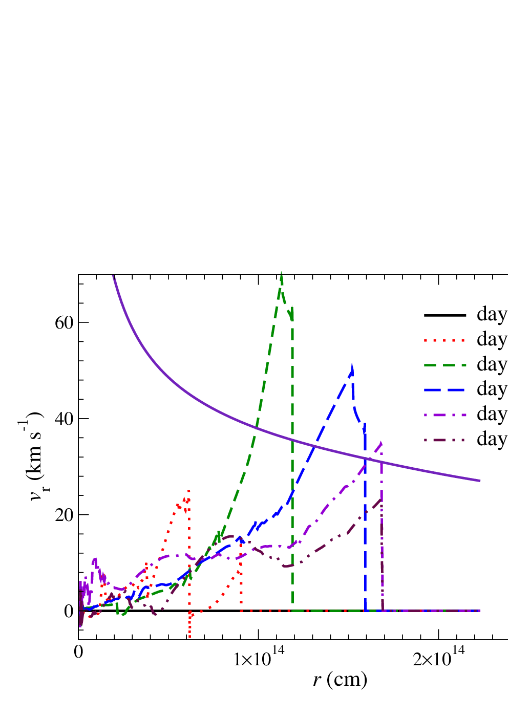
In Figure 9, we plot the velocity profiles of the MEM. Similar to the density profiles, the velocity profiles also show interesting differences between the two models. Model 2 with a low heating rate does not show deceleration, and the star reaches nearly homologous expansion at the end of simulation. Model 6 shows almost the opposite behavior. The energy injection creates a two-peak shock structure at day 114, with the inner shock traveling faster than the outer. The shocks merge into a stronger shock at day 228 that reaches above 60 km s-1, almost 50 % higher than Model 2, despite the same total energy deposited. However, the expansion is not sustained by further heating, and the surface velocity drops by half and reaches km s-1 at the end of the simulation.
4.1.3 Hydrodynamics of High-Energy Models
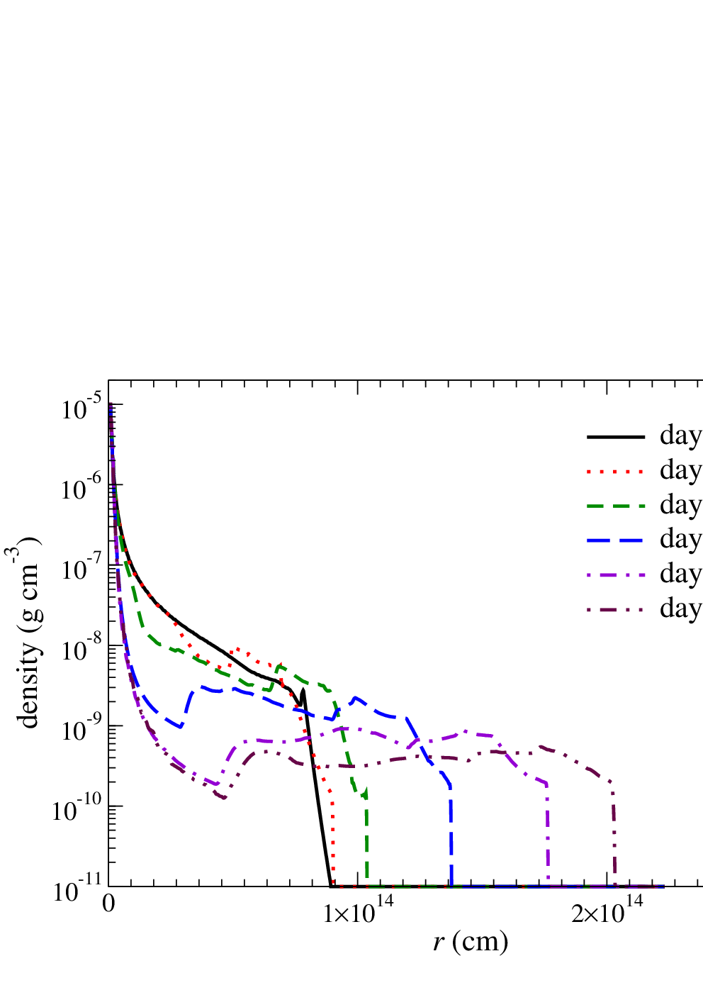
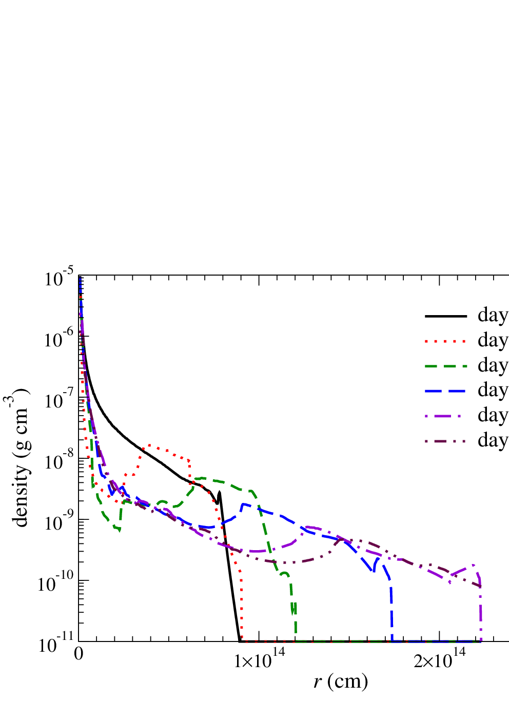
We next examine the HEM, Models 5 and 7, which have a higher deposited energy of erg. Figure 10 shows that the density profiles are drastically altered by the large energy deposition. Both models develop large density inversions as material in the inner envelope is lifted outwards. In Model 5, which has a lower , the density profile is flattened, with a density peak near cm at day 114 that propagates to nearly cm by day 570. In Model 7, the higher heating rate drives a stronger shock that expels material to larger radii. At day 456, the outer layers of the star reach the simulation outer boundary at cm.
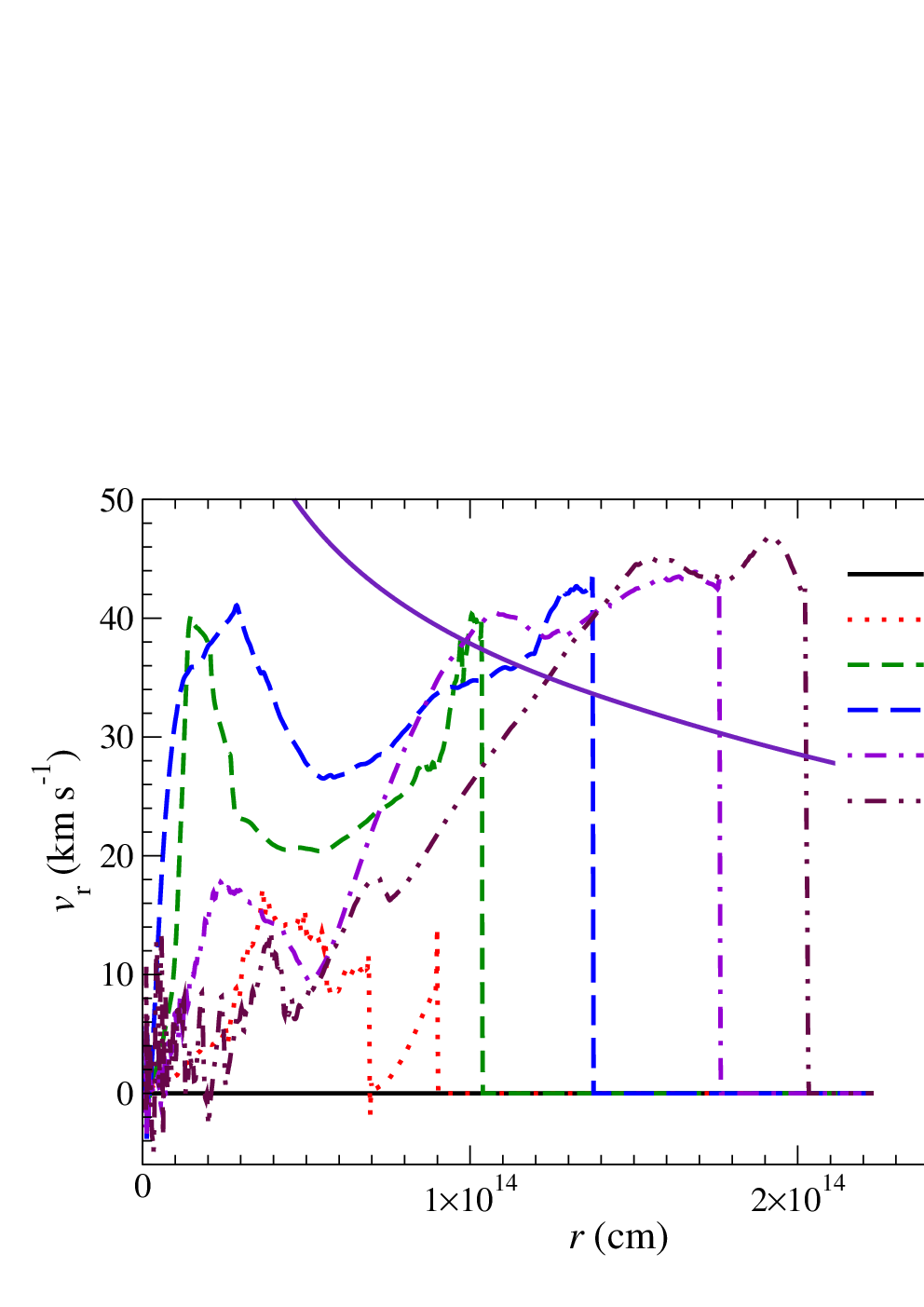
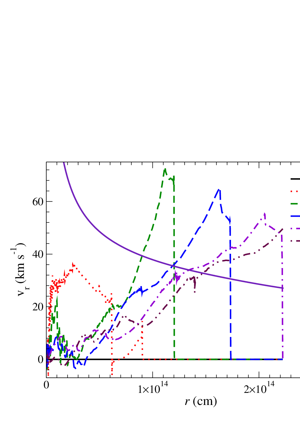
In Figure 11, we plot the velocity profiles of Models 5 and 7 from the HEM series. Model 5 shows that the star can still expand rapidly with a moderate but with a long duration. The velocity profile features a strong two peak structure at intermediate times but approaches homologous expansion at late times. The outer layers asymptotically approach a velocity km s-1, larger than the escape speed. The inner layers slows down with time, developing a complex turbulent structure in the core.
Dynamical features accompany the expansion in the velocity profiles of Model 7. When the strong shock breaks out from the surface of the star around day 228, the velocity peaks at 70 km s-1, compared to the local escape velocity of km s-. Afterwards, the ejecta slows down but can still escape. Turbulent motion persists in the inner part of the star. The outer layers of the ejecta reach the outer boundary of the simulation as shown in the profile at day 456. At the end of the run, the star approaches homologous expansion.
4.2 Dependence on Wave Heating Rate and Duration
In this Section, we discuss general differences between models with the same wave heating rate but different duration, or vice versa. The duration is determined by the lifetime of the core burning. The duration of the advanced burning, such as O-burning, generally decreases with stellar mass. The exact heating rate is also unclear as there is significant uncertainty in the wave luminosity generated by the convective core, but it is expected to increase for more massive stellar cores. Here, we explore the consequences of the variation of these values on the mass ejection process.
We examine how affects the evolution of the velocity profile by analyzing the three Models with a heating duration of 120 days: Model 1 (LEM), Model 4 (MEM), and Model 7 (HEM). The energy deposition rate significantly affects how the star expands and how the star ejects mass. A lower , makes the star expand but with no mass ejection. Higher values of can drive stronger shocks that lead to mass ejection from the surface. Only Model 7 with exhibits significant mass ejection due to wave heating. The larger energy deposition of the HEM not only makes the star expand faster, but it also creates a prolonged trough in the density profile inside the star. In contrast, the LEM exhibits very little internal motion or mass ejection in its velocity profile.
We identify significant differences in the density and velocity structures between models with different heating rates. Models with low but sustained heating rates exhibit more steady expansion, with a small density inversion forming as the outer layers are gradually lifted outwards by the expanding inner layers. Due to the low heating rate, no strong shock wave is excited, and matter is not shock-accelerated near the surface. We refer to this as a “bubble” phenomenon. In contrast, a larger heating rate excites a stronger shock that accelerates the surface layers outward, creating a low-density tail of material above the previous location of the photosphere, with a much smaller density inversion interior to this tail. We refer to this as a “bomb” phenomenon. Thus, low heating rates create a “bubble” phenomenon, while high heating rates (i.e., a heating time scale shorter than the local dynamical time scale) create a “bomb” phenomenon.
4.3 Global Comparison of Mass Loss
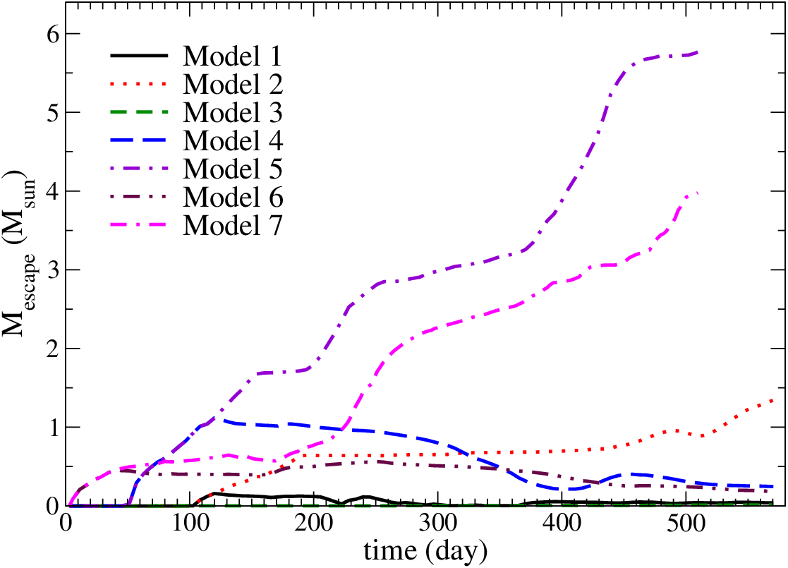
In Figure 12, we plot the total ejecta mass against time for the models presented. The ejecta mass is defined by the integrated mass elements when the sum of the local kinetic energy, internal energy and the potential energy is positive. This quantity is therefore time-dependent as demonstrated in previous sections. The 7 models can be characterized into three groups based on the total energy deposition: LEM models exhibit little to no mass loss, MEM models exhibit moderate amounts of mass loss, and HEM models exhibit large amounts of mass loss. For LEM (Models 1 and 3), effectively there is no ejected mass as the escape mass is as low as . The MEM (Models 2, 4, and 6) shows the ejected mass is roughly an order of magnitude higher at 0.5–1.5 . At last in HEM (Models 5 and 7), the ejected mass reaches asymptotic values of 4–6 , where the whole envelope mass is also .
The heating rate also affects the evolution of the ejected mass. Unsurprisingly, models with the largest heating rates (Models 6 and 7) show the fastest initial increase in unbound mass, while models with the lower heating rates require a longer time for any mass to accumulate enough energy to escape. Between models with the same energy deposition, lower heating rates with longer durations generally produce larger ejecta masses.
4.4 Global Comparison of Deposition Radius
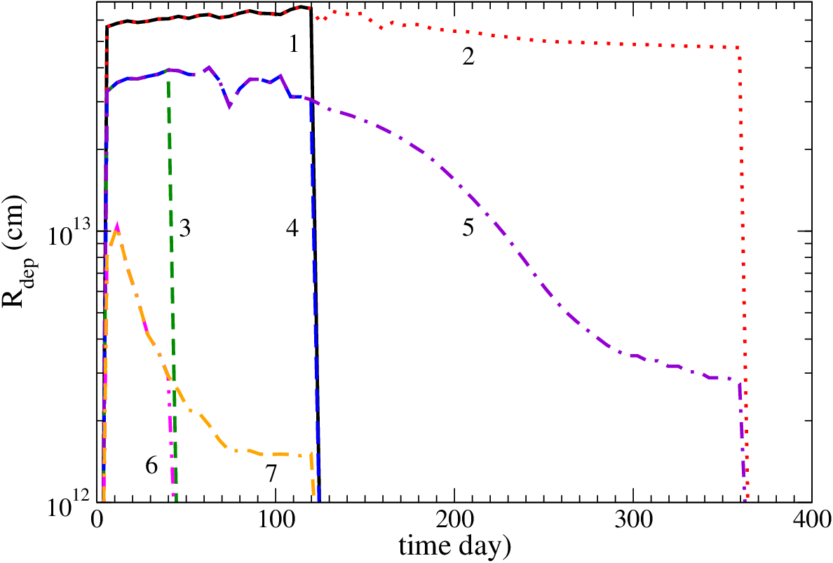
Here we compare the position where the acoustic waves deposit energy. In Figure 13, we plot the position of the energy deposition against time for the models presented. The sharp drop in all curves occurs when heating abruptly shuts off. We see that models with a lower have their energy deposition at larger radii, which differ from cm in Models 1 and 2, down to cm for Model 7. As the acoustic waves deposit their energy only when the maximum wave energy flux is exceeded (equation 1), a lower energy deposition rate requires a lower density and sound speed to match this criteria, so the heating occurs at larger radii. The roughly constant heating radius in Models 1–5 before day 100 suggests the wave energy does not strongly alter the stellar structure in the wave heating region during this time. The trends in the heating radius are correlated with , because the wave heat causes the inner envelope to expand and decrease in density, causing the heating radius to move inward. This happens almost immediately for the largest heating rates. As seen in Models 5 and 7, the recession of the deposition sphere can reduce its size by almost an order of magnitude.
4.5 Global Comparison of Energy

At last, we compare the total energy as a function of time among all models, plotted in Figure 14. Unsurprisingly, the final energy is mostly determined by the total acoustic wave energy deposition. Note that only Models 5 and 7 finish with positive total energy, implying large amounts of unbound material, as verified by the results in Figure 12. However, as the star expands, extra contributions of energy emerge due to the energy content of inflowing/outflowing matter across the simulation boundaries, so the final energy in the simulation is not merely the sum of the initial energy and the heating energy.
This is not just an artifact of the simulations, as mass in a real star will generally flow from below the wave heating region to above it, changing the net energy content of the envelope. This effect is negligible for models with lower , due to a smaller contribution from material flowing across the boundaries. Models with larger heating rates drive material away from the inner boundary, causing more matter to flow into the simulation domain from the inner boundary, which advects negative gravitational energy into the simulation domain.
In model 5, there is a mild increase of energy between day 400-450. This is the period when the rapid expansion creates an energy discontinuity near the isothermal outer layer, which is set to be at the minimum temperature allowed in the simulation ( K). When the discontinuity passes across this region, fluid elements can be cooled below the minimum temperature. In this code we choose to stick with thermodynamical consistency instead of energy consistency, so the missing energy between the actual temperature and the temperature floor is added into the system. Since this only alters the total energy budget by about , we do not believe it qualitatively affects our conclusions.
5 Discussion
5.1 Pre-supernova Mass Loss in Stars of Other Masses

In general, the outburst process depends strongly on the wave excitation in the core, in addition to the properties of the envelope, and both core and envelope should be evolved together for robust estimates. Fortunately, most red supergiant envelopes have very similar, nearly poltropic structures. The envelope masses are also similar, , since higher mass stars have more of their mass in their cores, and lose more envelope mass by winds. In contrast, stars of different mass have very different wave heating rates and heating durations (Shiode & Quataert 2014). Hence, in our parameter study, lower values of for longer durations are more representative of low-mass stars, while higher values of for shorter durations are more representative of high-mass stars. Different burning phases behave similarly: carbon shell-burning can be much longer ( years) but the wave luminosity is correspondingly smaller. Silicon burning generates much larger wave fluxes but only lasts days, so the envelope does not have time to respond Fuller et al. 2015.
It is possible that other processes occur in some stars, such as convective shell mergers. These would spur intense nuclear burning and vigorous convection (Meakin & Arnett 2006; Collins et al. 2018; Yadav et al. 2020), driving very large wave fluxes into the envelope. Another scenario is that the core dynamo amplifies the magnetic field in the convective shells near the core, which could also generate waves and lead to energy deposition near the surface (Soker & Gilkis 2017). While we do not investigate such processes here, an uncommon subset of stars could generate wave fluxes much greater than our fiducial estimates.
5.2 Appearance of Wave-driven Outbursts
Our simulations do not include radiative transfer and cannot predict the detailed appearance of wave-driven pre-SN outbursts. From the 1D models of Fuller 2017, the photometric signal of a pre-SN outburst in a red supergiant is likely dominated by shocks propagating up to the photosphere after short but intense periods of wave heating, such as the core neon burning phase. Our 2D simulations with large heating rates also launch these shocks, which are not strongly affected by non-radial instabilities. Hence, we expect that the observable features of pre-SN outbursts are captured reasonably well by 1D models. When the outburst takes place in a binary system, the accretion of the ejected matter by the companion star might also produce a bright event (Mcley & Soker 2014; Danieli & Soker 2019).
5.3 Envelope Asphericity

In this work, we have extensively computed two dimensional models showing how the wave heating generates asphericity and drives mass loss. In Figure 15, we further demonstrate how the asphericity develops at late times. We examine Models 2 and 6, finding that both models are spherical to a good approximation. However, notable turbulence is driven within the middle of the envelope, which is especially evident at at radii around cm. These structures are much more pronounced in Model 6, likely because the larger heating rate (but shorter duration) fuels more expansion of the inner envelope, generating stronger Rayleigh-Taylor instability. Furthermore, the density profile in Model 2 shows observable “wrinkles”, though it is not yet clear if these features are real or numerical artifacts. For LEM and MEM, the asphericity is small, and the wave heating primarily contributes to a quasi-spherical expansion of the stellar envelope.
For comparison, we also plot in Figure 16 the density color plots of two higher energy models, Models 5 and 7. The most striking features of these models is the large-scale structure with three wavelengths per quadrant at radii around cm. This is clearly a consequence of the initial configuration of the simulations, where a sinusoidal perturbation with three periods in the radial and angular directions (and an amplitude ) was embedded in the density profile. However, by the end of the simulation, this perturbation has grown to a large amplitude, producing as much as a factor of 10 variation in the horizontal density fluctuations. We attribute this large amplification to rapidly growing Rayleigh-Taylor instability. Interestingly, the radial location where the instability is most prominent depends on the wave heating rate, but it is clear that higher total heat deposition allows for more growth of density perturbations. Of course, a real star would have initial density fluctuations at a variety of scales due to turbulent convection in the envelope, but these models indicate those perturbations can be magnified by wave heating effects, potentially producing significant asphericity in the exploding star.
To quantify the level of asphericity in the models, we compute define the mass-weighted asphericity via the Fourier modes
| (2) |
Here, the integer is the Fourier harmonic and is the total mass of the star. We also compute a similar expression with using as the Fourier component, and we thus define the asphericity of -th order, .


In Figure 17 we plot the time evolution of the asphericity modes and of all 7 models presented in previous sections. The component is often dominant as discussed above. Comparing the two plots, is indeed smaller than by a factor of a few. The LEM show a mild increase in asphericity, but their low values show the stars remain nearly spherical. The MEM show a larger asphericity that grows nearly linearly in time. The HEM have the most significant asphericity, with the component of Model 7 reaching 10 %. Despite its lower total energy deposition, Model 5 exhibits the largest value of and hence has the most elongated structure, though the elongation only reaches . The angular dependence of the envelope density may give rise to interesting effects for the subsequent SN and its appearance.
In Appendix B we further compare models with different initial aspherical seeds to see how this affects the star’s final asphericity, finding the results are not strongly dependent on this choice.
5.4 Limitations of This Work
First, our simulations use a moderate resolution which is almost constant throughout the star with cm. This is rather large compared to the mass cut which is cm. Thus, the inner features of the star might not be fully captured and may be under-resolved. This value of can provide us the necessary resolution for the outer part to keep track of the smaller features due to hydrodynamical instabilities. Most such features should be produced in the outer envelope as that is the place where the density inversion is present.
Second, our simulation does not resolve the acoustic waves emitted from the core, instead only including a heating term to account for their energy deposition. Studying how these waves deposit heat and momentum is numerically challenging because it takes place on a short length and time scale, i.e., the wavelength and wave period. The huge number of acoustic waves leaked into the envelope provides the possibility of modeling this process statistically, namely by the recognition of as a time-averaged quantity. Interestingly, our results imply the net effect is for acoustic waves to damp via weak shocks, converting their energy into pressure pulses with larger length and time scales, which then continue to propagate out until they shock again. It would be an interesting extension to resolve both the original acoustic waves and the secondary pressure pulses to see if the results differ from the treatment adopted here.
Third we have used the Helmholtz equation of state for our computation. But for modeling the envelope, we are approaching a density close to g cm-3, which is the density floor provided by the equation of state table. As discussed above, the temperature would also decrease below K if we did not impose a temperature floor. This limits us to explore further how the ejecta behaves beyond day 570. In some of our more energetic models, vacuum zones develop inside the star, with a few grid cells along the same reaching the density floor. These are not evident in the figures because the density profiles shown are angle-averaged. The large associated pressure differences begins to trigger unphysical flow. Further extrapolation to lower densities and temperatures will require an updated equation of state. Additionally, at these low densities, the matter might not be tightly coupled to the radiation field, so non-diffusive radiative transfer may be important. Furthermore, the ionization state can be out of thermodynamical equilibrium. These factors might largely complicate the computations and these extra physics will be interesting follow-up work.
The density floor is set to maintain code stability when calling the equation of state. However, the presence of such a floor also sets a minimum mass which can be resolved in our simulation. To estimate that, we consider the outermost grid cells used in our simulation, located at a radius cm. Using the density floor, the minimum mass traceable by this grid is . The corresponding masses for inner grids are smaller as the grid volume scales as . This means the ejected mass ranging from in our models is likely well resolved by our code. For ejecta masses , a suitable extension to even lower density below g cm-3 will be necessary. However, extending to lower densities will also require additional physical considerations, such as the validity of thermodynamic equilibrium and the inclusion of radiative processes.
Fourth, our two-dimensional simulations might underestimate small-scale turbulent features. Hydrodynamical instabilities, such as the Kelvin-Helmholtz instabilities and Rayleigh-Taylor instabilities, can extend to the Kolmogorov length scale, where the viscous nature of the fluid becomes prominent. In fact, for a three-dimensional model, the development of Rayleigh-Taylor instability can be different because the extra dimension allows an extra degree of freedom for the development of the smaller features. This phenomenon is frequently seen in large-scale eddy modeling where two-dimensional and three-dimensional turbulent energy cascades have different energy flow direction. However, the large-scale features reported here should be similar in the two types of simulations.
Fifth, we do not consider the effects of recombination and radiative transfer in these simulations. In our progenitor model, the outer has an optical depth , hence the assumption of high optical depth in those layers is not very good. While the approximation of radiation being in equilibrium with matter is well maintained in the rest of the star, the true ejecta mass of our less energetic models (with ) may be reduced if radiation can leak out before their outer layers are accelerated toward the escape speed.
The effects of recombination can also potentially affect the expansion of the envelope. Our equation of state does not include recombination energy, and the ionization temperature of 4He (29000 K) and 1H (10000 K) overlaps with the temperature range used in the simulation, meaning that partial recombination should take place during its expansion. Because of the envelope’s low binding energy, this energy contributes substantially to the energy budget, and it may drive greater envelope expansion and mass loss than predicted by these simulations. On the other hand, recombination reduces the envelope opacity, allowing thermal energy to leak out, as described above. Resolving this competition between energy deposition by recombination, and energy loss by radiation, will be needed for better estimates of the mass loss and pre-SN density profile.
Sixth, in the simulations we have made approximations for the initial conditions and energy deposition. In fact, how the exact energy deposition takes place in such a thin mass slice, and how the initial convective structure can be coupled to a hydrostatic model, should be further explored.
To clarify how these limitations affect the final results, we provide in the appendices more comparison tests. In Appendix A, we study how the initial density perturbation affects the later evolution without energy deposition. In Appendix B, we examine how the choice of density perturbation affects the later evolution. In Appendix C, we further compare how our two-dimensional energy deposition differs from the previous reported one-dimensional energy deposition model in Fuller 2017. In Appendix D, we study how our choice of smearing mass for the energy deposition affects the morphology and dynamics of the ejecta. In Appendix E, we provide further details on our coordinate system. The above tests aim for clarifying the physics necessary for a comprehensive parameter survey for our future work.
5.5 Conclusion
In this work, we study the multidimensional hydrodynamical response of a red supergiant envelope heated by wave energy transport from nuclear burning in the core. We extract the stellar envelope from a 15 stellar model, and we inject energy similar to that expected from the wave luminosity and duration of the core oxygen-burning phase. To understand sensitivity to the uncertain wave luminosity and duration, we treat the heat deposition rate and its duration as model parameters. Unsurprisingly, we find that heat deposition in excess of the envelope’s binding energy can drive large amounts of mass loss, while heat deposition lower than this threshold has a much smaller impact.
We also observe two classes of behaviors that depend on the wave heating rate. For a lower wave energy flux, the wave energy causes gradual expansion of the stellar envelope without strong mass loss, and the expansion is mostly spherical. With a high wave energy flux, the wave energy can amplify initial density asphericities and trigger uneven heating. This results in more asymmetric motion in the envelope where the Rayleigh Taylor instability arises, smoothing radial density inversions that occur in one-dimensional models. Larger heating rates also drive stronger shocks, expelling material above the original photosphere of the star. These low-density tails above the star’s photosphere may have important effects on the early light curves of Type II-P SNe. Such events would also likely lead to observable pre-SN outbursts.
Comparison between our two-dimensional models and spherically symmetric models show only modest differences, mostly arising from Rayleigh-Taylor instabilities that smooth out density inversions created by wave heating. Hence, one-dimensional models are likely to yield reasonably good estimates of the unbound mass and the photometric signals produced by pre-SN outbursts in red supergiants. However, multi-dimensional models or one-dimensional models incorporating effects of Rayleigh-Taylor instability (Duffell 2016) should be used for estimates of the pre-SN density profile.
We further discuss how the results of this work can be applied to stars of different mass. More massive stars with more vigorous convection during oxygen burning can potentially result in large enough heating rates to launch shocks which trigger observable outbursts and mass loss from the stellar envelope before the star collapse. Less massive stars with lower wave heating rates are unlikely to suffer such outbursts, except in cases where degenerate burning flashes, convective shell mergers, or a different core structure permit larger wave fluxes into the envelope. The corresponding optical signal, and the implications for SNe light curves will be interesting follow-up work.
6 Acknowledgments
We thank Paul Duffell for useful insight regarding the simulations and results. S.C.L. acknowledges support from grants HST-AR-15021.001-A and 80NSSC18K1017. JF is thankful for support through an Innovator Grant from The Rose Hills Foundation, and the Sloan Foundation through grant FG-2018-10515. We thank Frank X. Timmes for his open-source subroutines for the Helmholtz equation of state and the template for the 7-isotope nuclear reaction network. We also thank the developers of the stellar evolution code MESA for their efforts in making the code public.
MESA (v8118); (Paxton et al. 2011; Paxton et al. 2013; Paxton et al. 2015; Paxton et al. 2017)
Appendix A Initial Model
In building the initial model, we have used the hydrostatic model computed by the MESA code as the input. We map the one-dimensional data, containing the temperature and chemical composition as a function of the mass coordinate and radial distance, onto a two-dimensional polar grid by solving again the hydrostatic equilibrium equation for the density profile. Here we check how the initial model varies with time when there is no energy deposition. This helps us understand whether the inner mass cut and the mapping satisfies the hydrostatic equilibrium. It also serves as a reference for how much the initial aspherical seed contributes to the initial motion.


In Figure 18 we plot in the left and right panels the density and radial velocity profiles of the test model. The initial model is exactly the same as those used in the main text, but without any energy deposition during the simulation. From the density profiles, we can see that the star gradually relaxes to a new equilbrium that is slightly different from the initial conditions. The star mildly expands, indicated by the mild drop of the density at cm and the outward motion of the surface. By the end of the simulation, the sharp cliff in density at the photosphere, originally at cm, is partially smoothed out.
From the velocity profile, we can see the initial conditions do create some internal motion, leading to radial velocities of km s-1, which is much lower than the escape velocity at km s-1. However, by comparing with the models from the main text, we can see the motion is much smaller than those with even low amounts of energy deposition, such as Model 3. Those models have a final radius of – times of the initial radius, while the test model only expands by . Hence, we can be confident that the majority of the response in the heated models is due to the deposited energy, as opposed to artifacts of the initial conditions
Appendix B Effects of Initial Aspherical Seeds
In the main text, we have described how we added density perturbations as a source of initial asphericity for enhancing the later development of aspherical motion and instabilities. We used a somewhat arbitrary value of . However, the actual density perturbations due to convection would certainly be different.
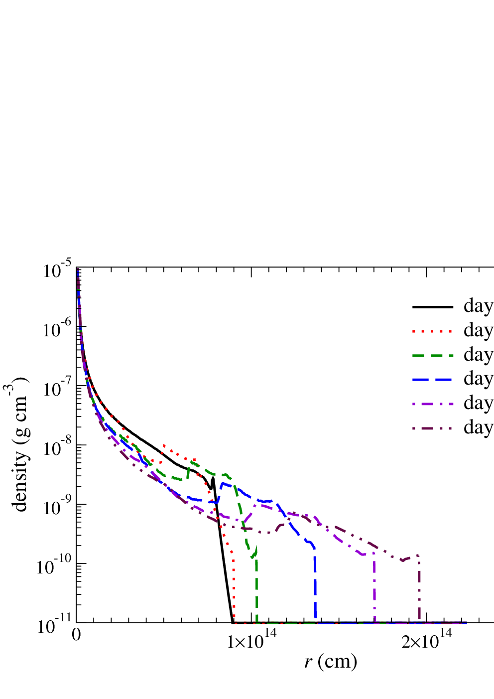
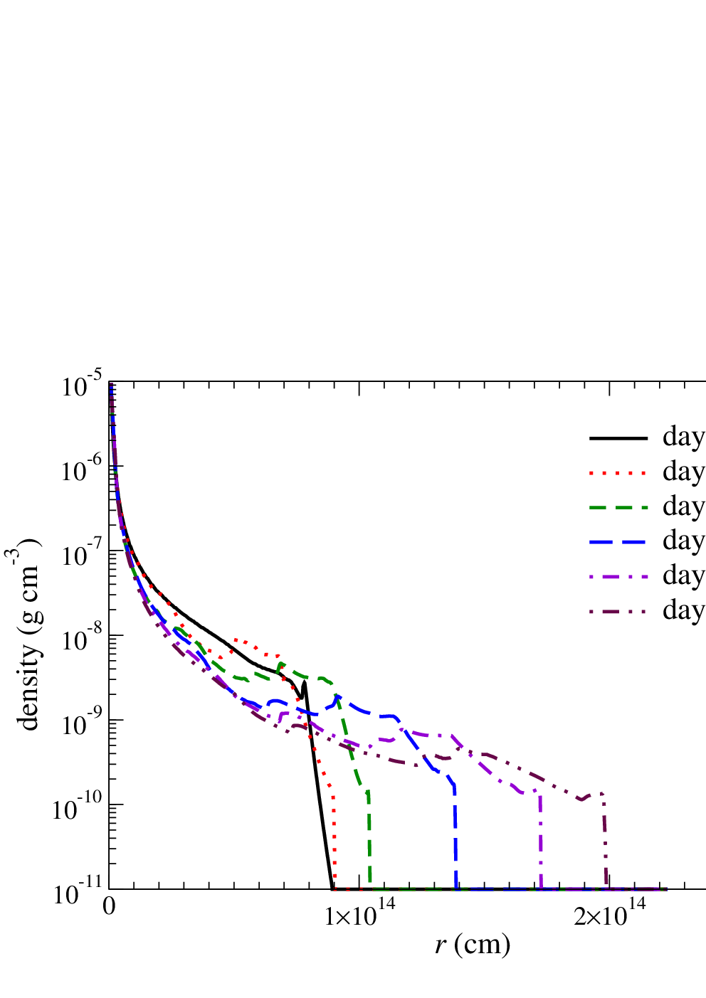
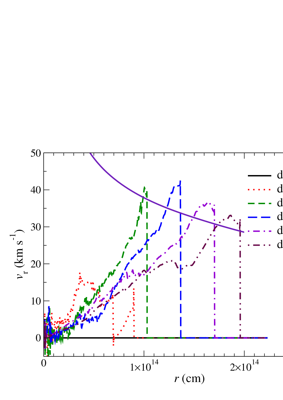
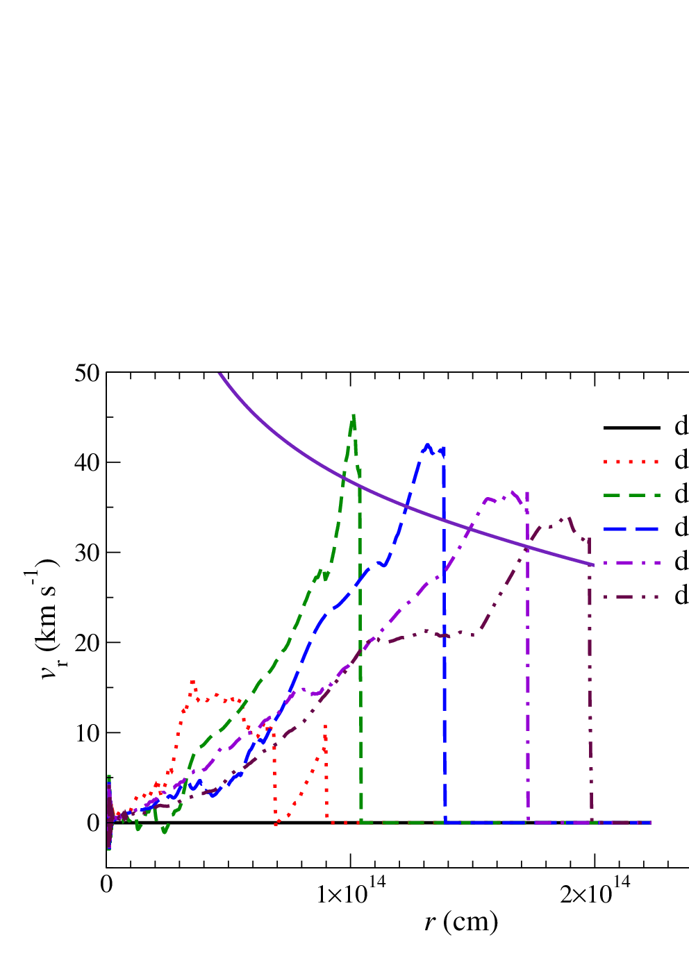
Here we examine how the initial density perturbation affect the energy deposition. We do not perturb the velocity fields because we find that the vector nature of the velocity is more difficult to construct a good profile provides a good conservation of mass throughout the star, where density spans more than 6 orders of magnitude. In Figure 19 we plot the density, and velocity for two models identical to model 4, but with initial density perturbations smaller and larger by an order of magnitude. In both models, the behavior is very similar to that of Model 4. The similarity of the density profiles give us indicates that most of our results are insensitive to the details of the asphericity and density perturbations that would be present in a real star.
The velocity profiles of these models further indicates insensitivity to the initial density perturbations. Comparing the profiles of two models at the same time slice, the differences are only . The similarity of the velocity profiles also ensures that our main results are robust against our choice of initial conditions.


For comparison, we also compute a model without any initial density perturbations, shown in Figure 20. Interestingly, this model shows a stiffer structure than our previous models, more akin to the one-dimensional models of Fuller 2017. The density inversion is slightly larger and with a steeper boundary, likely because the initial spherical symmetry results in Rayleigh-Taylor instabilities that take longer to grow and smooth it out. We also computed the Fourier asymmetry components, and they are a few orders of magnitude lower than our models presented in the main text. The velocity profiles in the right panel of Figure 20 are very similar to the models with density perturbations. We conclude that density perturbations should be added to capture the realistic growth of Rayleigh-Taylor instabilities, but that the magnitude of the perturbations do not strongly affect our results. Furthermore, we remark that in this simulation, the spherical symmetry is strictly preserved that the polar velocity field remains zero throughout the simulation. This ensures us that the simulation is equivalent to the one-dimensional simulation counterpart that the pressure at a constant-radius slice is always balanced such that no spurious polar flow can be triggered when the model starts with spherical symmetry.
Appendix C Effects of Energy Deposition Mass
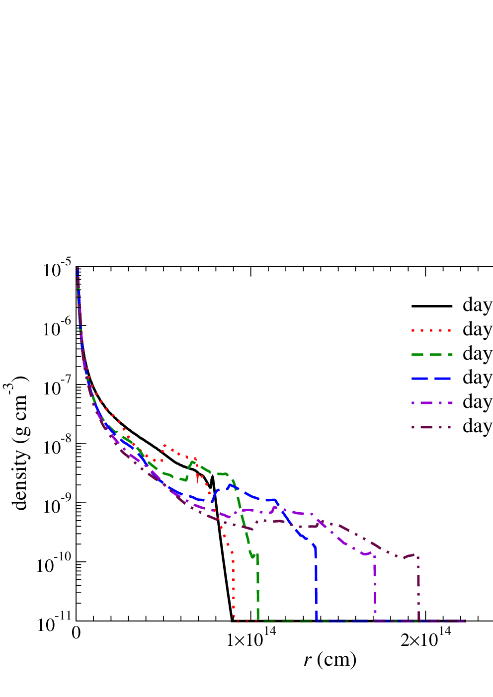
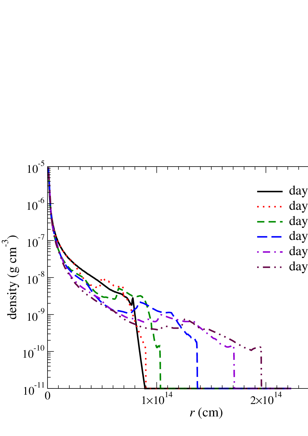

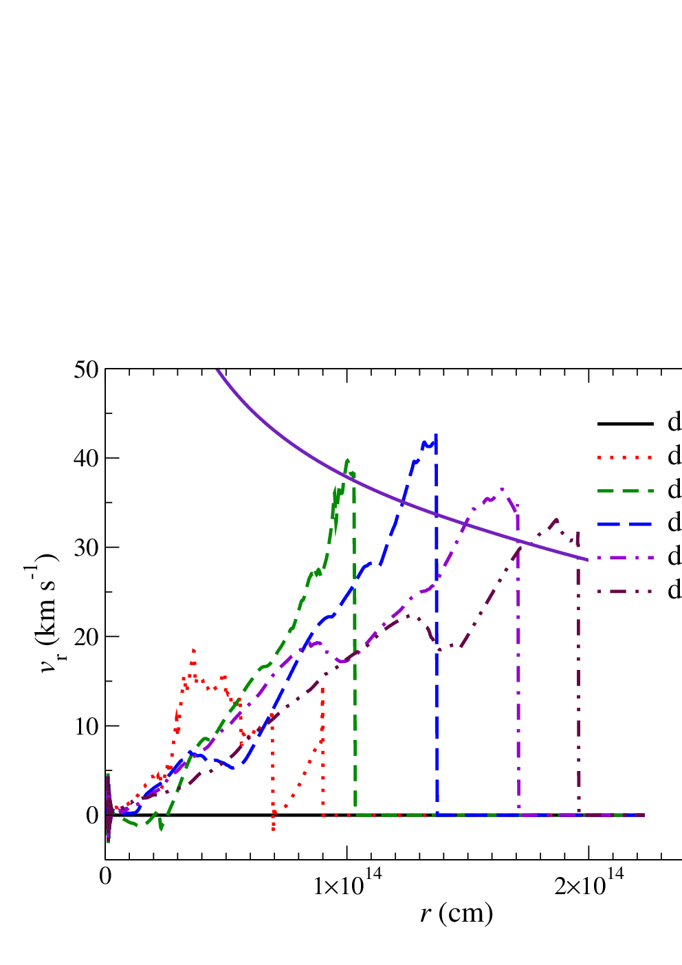
Here we compare how the choice of smoothing the energy deposition over mass affects our results. When we calculate how the waves deposit the energy, we always smear the full energy deposition into a mass of because in extreme cases the deposition sphere can recede towards the inner boundary. This poses a challenging modeling scenario as the sharp drop of the density and sound speed profile can cause all the energy to be deposited in a single grid cell, such that the energy deposition is not well resolved. In fact, for the higher case (), the deposition length scale can become much smaller than a grid cell, so it is numerically impossible to resolve the exact distribution of energy. To alleviate the problem, we define such that the energy deposition is always smeared into a few grid cells, such that our results are less sensitive to resolution.
To test the effect of this parameter on our results, we perform two extra models, Model 4c and Model 4d, which have and respectively. In Figure 21, we plot the density and velocity profiles for the two models. Despite the fact that the deposition mass differs by 4 times between the two models, we can see that there are almost no observable differences, except minor changes in the peak velocity and the details of the density gradient. This provides evidence that the smearing procedure provides a good enough description for the energy deposition process in a resolvable manner.
Appendix D Global Comparison of Test Models

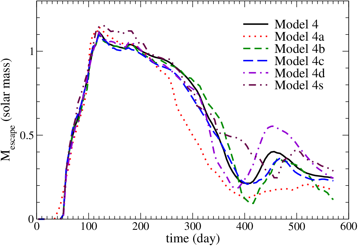
Next, we compare the global energetics and the ejecta mass for the test cases examined in the appendix. They serve as a general diagnostic as how sensitive each controllable parameter is to our final result. In Figure 22, we plot the total energy and its components for the test models, including Model 4 as a reference. We also plot the ejecta mass as a function of time. We can see that the choice of or aspherical seed size does not significantly change the energetics of the star. Model 4s shows a slightly larger expansion as described in above, thus it has a slightly higher potential energy due to more energy inflow from the atmosphere.
In regards to the ejecta mass, Figure 22 shows that all the models are qualitatively the same, suggesting that the ejecta mass is not sensitive to the parameters presented above. All models show their peak at Day 120 at and then the unbound mass gradually decreases until day 400 at 0.1–0.4 . At that point the models begin to deviate somewhat, but the final ejecta mass is always in the range 0.1–0.3 .
Appendix E Notes on the Geometry
Our wedge simulations can be considered to be pieces of the star’s equatorial or meridional plane. We use periodic boundary conditions in so that matter leaving one boundary enters the other boundary. For the computations of mass and energy, we define the volume elements for a quadrant, automatically giving the volume of a sphere when integrated in both and . In this choice, the 2D grid cells are intersections of 3D volume elements with the orbital plane, with each 3D volume element wrapping from the positive -axis to the negative -axis at constant radius. In the literature, axisymmetric models in the meridional plane are more frequently used for two-dimensional simulations. In the absence of rotational symmetry breaking forces, our geometry is physically identical to the meridional plane. We choose this geometry over a meridional plane geometry (in which case the volume elements would be ) to give equal weight to all latitudes . Additionally, we choose periodic boundary conditions because a closed boundary in the polar direction can strongly suppress the polar flow in the simulation.
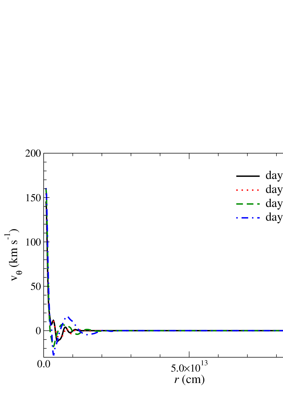
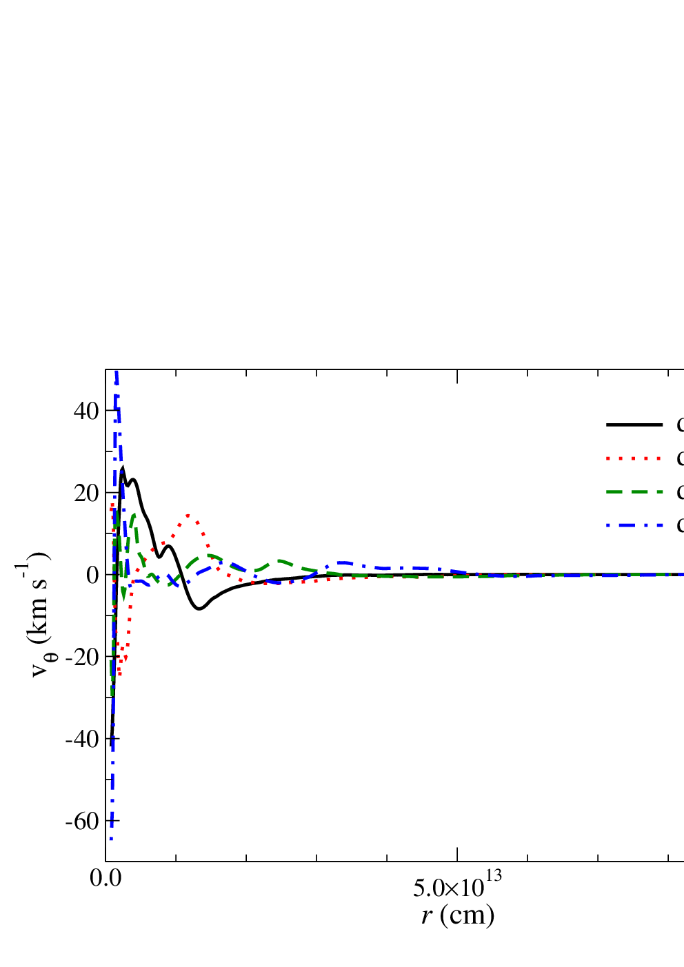
In the main text, we noted that the energy deposition may generate a substantial horizontal flow in the inner layers of the star. To examine the choice of boundary conditions on this flow, we recompute Model 4 with reflective angular boundary conditions, explicitly suppressing any flow across those boundaries. We show in Figure 23 the angular velocities in both cases. In the model with periodic boundaries, a high-velocity flow has developed and remains substantial from day 114. On the other hand, the model with reflective boundaries shows lower velocities near the inner boundary, but similar velocities everywhere else. While the heating may drive mean flows in the inner layers, the angular motion appears turbulent in the outer part of the domain. The two models indicate that the dynamics of the outer part of the star are insensitive to the boundary conditions, but the possibility of rotational flows in the inner part of the star should be examined in future work.
References
- Alvan et al. (2015) Alvan, L., Strugarek, A., Brun, A. S., Mathis, S., & Garcia, R. A. 2015, A&A, 581, A112
- Barth & Deconinck (1999) Barth, T. J., & Deconinck, H. 1999, Lecture Notes in Computational Science and Engineering 9: High-Order Methods for Computational Physics (Springer)
- Collins et al. (2018) Collins, C., Müller, B., & Heger, A. 2018, MNRAS, 473, 1695
- Corsi et al. (2014) Corsi, A., Ofek, E. O., Gal-Yam, A., et al. 2014, ApJ, 782, 42
- Danieli & Soker (2019) Danieli, B., & Soker, N. 2019, MNRAS, 482, 2277
- Duffell (2016) Duffell, P. C. 2016, ApJ, 821, 76
- Elias-Rosa et al. (2016) Elias-Rosa, N., Pastorello, A., Benetti, S., et al. 2016, MNRAS, 463, 3894
- Fuller (2017) Fuller, J. 2017, MNRAS, 470, 1642
- Fuller et al. (2015) Fuller, J., Cantiello, M., Stello, D., Garcia, R. A., & Bildsten, L. 2015, Science, 350, 423
- Fuller & Ro (2018) Fuller, J., & Ro, S. 2018, MNRAS, 476, 1853
- Gal-Yam et al. (2014) Gal-Yam, A., Arcavi, I., Ofek, E. O., et al. 2014, Nature, 509, 471
- Goldreich & Kumar (1990) Goldreich, P., & Kumar, P. 1990, ApJ, 363, 694
- Gräfener & Vink (2016) Gräfener, G., & Vink, J. S. 2016, MNRAS, 455, 112
- Groh (2014) Groh, J. H. 2014, A&A, 572, L11
- Ho et al. (2019) Ho, A. Y. Q., Goldstein, D. A., Schulze, S., et al. 2019, ApJ, 887, 169
- Johnson et al. (2018) Johnson, S. A., Kochanek, C. S., & Adams, S. M. 2018, MNRAS, 480, 1696
- Khazov et al. (2016) Khazov, D., Yaron, O., Gal-Yam, A., et al. 2016, ApJ, 818, 3
- Kochanek et al. (2017) Kochanek, C. S., Fraser, M., Adams, S. M., et al. 2017, MNRAS, 467, 3347
- Landau & Lifshitz (1959) Landau, L. D., & Lifshitz, E. M. 1959, Fluid mechanics
- Leung et al. (2015) Leung, S.-C., Chu, M.-C., & Lin, L.-M. 2015, Mon. Not. R. astr. Soc., 454, 1238
- Leung & Nomoto (2017) Leung, S.-C., & Nomoto, K. 2017, Proc. NIC2016, 14, 040506
- Leung & Nomoto (2018) Leung, S.-C., & Nomoto, K. 2018, ApJ, 861, 143
- Leung & Nomoto (2019) —. 2019, PASA, 36, e006
- Leung & Nomoto (2020) —. 2020, ApJ, 888, 80
- Leung et al. (2019a) Leung, S.-C., Nomoto, K., & Blinnikov, S. 2019a, ApJ, 887, 72
- Leung et al. (2020) Leung, S.-C., Nomoto, K., & Suzuki, T. 2020, ApJ, 889, 34
- Leung et al. (2019b) Leung, S.-C., Zha, S., Chu, M.-C., Lin, L.-M., & Nomoto, K. 2019b, ApJ, 884, 9
- Mauerhan et al. (2013) Mauerhan, J. C., Smith, N., Filippenko, A. V., et al. 2013, MNRAS, 430, 1801
- Mcley & Soker (2014) Mcley, L., & Soker, N. 2014, MNRAS, 445, 2492
- Meakin & Arnett (2006) Meakin, C. A., & Arnett, D. 2006, ApJ, 637, L53
- Mihalas & Mihalas (1984) Mihalas, D., & Mihalas, B. W. 1984, Foundations of radiation hydrodynamics
- Moriya et al. (2018) Moriya, T. J., Förster, F., Yoon, S.-C., Gräfener, G., & Blinnikov, S. I. 2018, MNRAS, 476, 2840
- Moriya et al. (2017) Moriya, T. J., Yoon, S.-C., Gräfener, G., & Blinnikov, S. I. 2017, MNRAS, 469, L108
- Morozova et al. (2020) Morozova, V., Piro, A. L., Fuller, J., & Van Dyk, S. D. 2020, ApJ, 891, L32
- Morozova et al. (2017) Morozova, V., Piro, A. L., & Valenti, S. 2017, ApJ, 838, 28
- Morozova et al. (2018) —. 2018, ApJ, 858, 15
- Ofek et al. (2013) Ofek, E. O., Sullivan, M., Cenko, S. B., et al. 2013, Nature, 494, 65
- Ofek et al. (2014) Ofek, E. O., Sullivan, M., Shaviv, N. J., et al. 2014, ApJ, 789, 104
- Ofek et al. (2016) Ofek, E. O., Cenko, S. B., Shaviv, N. J., et al. 2016, ApJ, 824, 6
- Ouchi & Maeda (2019) Ouchi, R., & Maeda, K. 2019, ApJ, 877, 92
- Pastorello et al. (2007) Pastorello, A., Smartt, S. J., Mattila, S., et al. 2007, Nature, 447, 829
- Paxton et al. (2011) Paxton, B., Bildsten, L., Dotter, A., et al. 2011, Astrophys. J. Suppl., 192, 3
- Paxton et al. (2013) Paxton, B., Cantiello, M., Arras, P., et al. 2013, Astrophys. J. Suppl., 208, 4
- Paxton et al. (2015) Paxton, B., Marchant, P., Schwab, J., et al. 2015, Astrophys. J. Suppl., 220, 15
- Paxton et al. (2017) Paxton, B., Schwab, J., Bauer, E. V., et al. 2017, Astrophys. J. Suppl., 234, 34
- Paxton et al. (2019) Paxton, B., Smolec, R., Schwab, J., et al. 2019, ApJS, 243, 10
- Quataert & Shiode (2012) Quataert, E., & Shiode, J. 2012, MNRAS, 423, L92
- Ro & Matzner (2017) Ro, S., & Matzner, C. D. 2017, ApJ, 841, 9
- Shiode & Quataert (2014) Shiode, J. H., & Quataert, E. 2014, ApJ, 780, 96
- Shivvers et al. (2016) Shivvers, I., Zheng, W. K., Mauerhan, J., et al. 2016, MNRAS, 461, 3057
- Shivvers et al. (2017) Shivvers, I., Zheng, W., Van Dyk, S. D., et al. 2017, MNRAS, 471, 4381
- Soker & Gilkis (2017) Soker, N., & Gilkis, A. 2017, MNRAS, 464, 3249
- Sorokina et al. (2016) Sorokina, E., Blinnikov, S., Nomoto, K., Quimby, R., & Tolstov, A. 2016, ApJ, 829, 17
- Takata (2016) Takata, M. 2016, PASJ, 68, 91
- Timmes et al. (2000) Timmes, F. X., Hoofman, R. D., & Woosley, S. E. 2000, Astrophys. J. Suppl., 129, 377
- Tolstov et al. (2017) Tolstov, A., Nomoto, K., Blinnikov, S., et al. 2017, ApJ, 835, 266
- Ulmschneider (1970) Ulmschneider, P. 1970, Sol. Phys., 12, 403
- Wang & Spiteri (2007) Wang, R., & Spiteri, R. J. 2007, SIAM J. Numer. Anal., 45, 1871
- Woosley (2018) Woosley, S. E. 2018, ApJ, 863, 105
- Woosley et al. (2007) Woosley, S. E., Blinnikov, S., & Heger, A. 2007, Nature, 450, 390
- Woosley et al. (2002) Woosley, S. E., Heger, A., & Weaver, T. A. 2002, Reviews of Modern Physics, 74, 1015
- Yadav et al. (2020) Yadav, N., Müller, B., Janka, H. T., Melson, T., & Heger, A. 2020, ApJ, 890, 94
- Yaron et al. (2017) Yaron, O., Perley, D. A., Gal-Yam, A., et al. 2017, Nature Physics, 13, 510
- Yoshida et al. (2016) Yoshida, T., Umeda, H., Maeda, K., & Ishii, T. 2016, MNRAS, 457, 351
- Zha et al. (2019a) Zha, S., Chu, M.-C., Leung, S.-C., & Lin, L.-M. 2019a, ApJ, 883, 13
- Zha et al. (2019b) Zha, S., Leung, S.-C., Suzuki, T., & Nomoto, K. 2019b, ApJ, 886, 22