跳到论文正文
W Papers独立论文阅读器 arXiv:2007.11567 论文正文 计算阅读时间 · 0%
引用这篇论文根据当前论文元数据生成,正式投稿前建议核对。


License: arXiv.org perpetual non-exclusive license
arXiv:2007.11567v2 [gr-qc] 23 Jun 2021

UFIFT-QG-20-04

Inflaton Effective Potential from Fermions for General ϵ\epsilon

A. Sivasankaran∗ and R. P. Woodard†

Department of Physics, University of Florida,
Gainesville, FL 32611, UNITED STATES

ABSTRACT

We accurately approximate the contribution of a Yukawa-coupled fermion to the inflaton effective potential for inflationary geometries with a general first slow roll parameter ϵ⁡(t)\epsilon(t). For ϵ=0\epsilon=0 our final result agrees with the famous computation of Candelas and Raine done long ago on de Sitter background [1], and both computations degenerate to the result of Coleman and Weinberg in the flat space limit [2]. Our result contains a small part that depends nonlocally on the inflationary geometry. Even in the numerically larger local part, very little of the ϵ\epsilon dependence takes the form of Ricci scalars. We discuss the implications of these corrections for inflation.

PACS numbers: 04.50.Kd, 95.35.+d, 98.62.-g

∗ e-mail: aneeshs@ufl.edu

† e-mail: woodard@phys.ufl.edu

1 Introduction

The most recent data on primordial perturbations [3] are consistent with the simplest models of inflation based on gravity plus a single, minimally coupled scalar inflaton φ\varphi,

ℒinflaton=R​−g16​π​G−12​∂μφ​∂νφ​gμ​ν​−g−V⁡(φ)​−g.\mathcal{L}_{\rm inflaton}=\frac{R\sqrt{-g}}{16\pi G}-\frac{1}{2}\partial_{\mu}\varphi\partial_{\nu}\varphi g^{\mu\nu}\sqrt{-g}-V(\varphi)\sqrt{-g}\;. (1)

Once inflation is established the system rapidly approaches homogeneity and isotropy, which means φ→φ0​(t)\varphi\rightarrow\varphi_{0}(t) and,

d​s2=−d​t2+a2​(t)​d​x→⋅d​x→⟹H⁡(t)≡a˙a,ϵ⁡(t)≡−H˙H2.ds^{2}=-dt^{2}+a^{2}(t)d\vec{x}\!\cdot\!d\vec{x}\qquad\Longrightarrow\qquad H(t)\equiv\frac{\dot{a}}{a}\;\;,\;\;\epsilon(t)\equiv-\frac{\dot{H}}{H^{2}}\;. (2)

Inflation proceeds as long as the inflaton’s potential energy dominates the nontrivial Einstein equations,

3​H2\displaystyle 3H^{2} =\displaystyle= 8​π​G​[12​φ˙02+V⁡(φ0)],\displaystyle 8\pi G\Bigl[\frac{1}{2}\dot{\varphi}_{0}^{2}+V(\varphi_{0})\Bigr]\;, (3)
−(−2​ϵ)​H2\displaystyle-(3\!-\!2\epsilon)H^{2} =\displaystyle= 8​π​G​[12​φ˙02−V⁡(φ0)],\displaystyle 8\pi G\Bigl[\frac{1}{2}\dot{\varphi}^{2}_{0}-V(\varphi_{0})\Bigr]\;, (4)

Hubble friction slows the inflaton’s roll down its potential,

φ¨0+3​H​φ˙0+V′​(φ0)=0⟹φ˙0≃−124​π​G​V′​(φ0)V⁡(φ0).\ddot{\varphi}_{0}+3H\dot{\varphi}_{0}+V^{\prime}(\varphi_{0})=0\qquad\Longrightarrow\qquad\dot{\varphi}_{0}\simeq-\frac{1}{\sqrt{24\pi G}}\frac{V^{\prime}(\varphi_{0})}{\sqrt{V(\varphi_{0})}}\;. (5)

At the end of inflation the scalar’s potential energy falls to become comparable to its kinetic energy, which reduces Hubble friction and allows φ\varphi to rapidly oscillate around the minimum of its potential. During this phase of “reheating” the inflaton’s kinetic energy is transferred into a hot, dense plasma of ordinary particles and Big Bang cosmology follows its usual course.

Facilitating the transfer of inflaton kinetic energy into ordinary matter during reheating obviously requires a coupling between φ\varphi and ordinary matter. The one we shall study here is to a massless fermion,

ℒfermion=ψ¯γbebμ(∂μ+i2Aμ​c​dJc​d)ψ−g−fφψ¯ψ−g.\mathcal{L}_{\rm fermion}=\overline{\psi}\gamma^{b}e^{\mu}_{~b}\Bigl(\partial_{\mu}\!+\!\frac{i}{2}A_{\mu cd}J^{cd}\Bigr)\psi\sqrt{-g}-f\varphi\overline{\psi}\psi\sqrt{-g}\;. (6)

where eμ​c​(x)e_{\mu c}(x) is the vierbein (with gμ​ν​(x)=eμ​a​(x)​eν​b​(x)​ηa​bg_{\mu\nu}(x)=e_{\mu a}(x)e_{\nu b}(x)\eta^{ab}), Aμ​c​d​(x)=ecν​(∂μeν​d−Γμ​νρ​eρ​d)A_{\mu cd}(x)=e^{\nu}_{~c}(\partial_{\mu}e_{\nu d}-\Gamma^{\rho}_{~\mu\nu}e_{\rho d}) is the spin connection, the γa\gamma^{a} are gamma matrices (with {γa,γb}=−2​ηa​b​I\{\gamma^{a},\gamma^{b}\}=-2\eta^{ab}I) and Jc​d≡i4​[γc,γd]J^{cd}\equiv\frac{i}{4}[\gamma^{c},\gamma^{d}]. Such a coupling causes the 0-point energy of ordinary matter (in this case, the fermion) to induce corrections to the inflaton potential V⁡(φ)V(\varphi) the same way that Coleman and Weinberg long ago demonstrated in flat space [2],

Δ​Vflat​(φ)=−(f​φ)48​π2​ln⁡(f​φs).\Delta V_{\rm flat}(\varphi)=-\frac{(f\varphi)^{4}}{8\pi^{2}}\ln\Bigl(\frac{f\varphi}{s}\Bigr)\;. (7)

(Here ss is the renormalization scale.) The result on an inflationary background (2) depends in a complicated way on HH and ϵ\epsilon — which we will elucidate — but expression (7) is still the leading large field result [4].

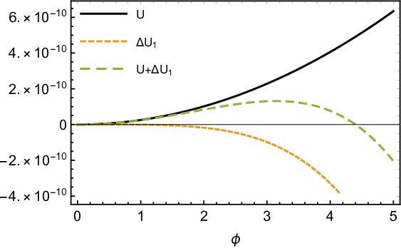
Cosmological Coleman-Weinberg potentials are potentially problematic for inflation because they can make significant changes to the classical trajectory of the inflaton [5]. To fully explore the problem requires the dependence upon HH and ϵ\epsilon that we shall determine, but the possibility of a problem is evident from the large field limiting form (7) which is plotted in Figure 1. Suppose the classical potential that drives inflation is the simple quadratic model, with its mass tuned to agree with the observed [3] scalar amplitude,

V⁡(φ)=c2​φ216​π​G,c≃7.1×10−6.V(\varphi)=\frac{c^{2}\varphi^{2}}{16\pi G}\qquad,\qquad c\simeq 7.1\times 10^{-6}\;. (8)
Refer to caption
Figure 1: The solid black line is the dimensionless classical potential U≡(8​π​G)2​V=12​c2​ϕ2U\equiv(8\pi G)^{2}V=\frac{1}{2}c^{2}\phi^{2} plotted as a function of the dimensionless inflaton field ϕ≡8​π​G×φ\phi\equiv\sqrt{8\pi G}\times\varphi. The dashed orange line is the one loop quantum correction for coupling f2=4.5×10⁻⁶f^{2}=4.5\times 10^{-6}, and the dashed green line is the total potential. Note that solving the Horizon problem in the classical model requires an initial value of ϕb<∼14\phi_{b}\mathrel{\raise 1.03334pt\hbox{$<$\kern-6.37509pt\lower 3.44444pt\hbox{$\sim$}}}14, at which point the total potential drives evolution towards a Big Rip singularity.

Although the classical trajectory of φ\varphi is towards zero starting from any initial value, the fact that fermionic corrections to the effective potential are negative means that a sufficiently large initial value drives the inflaton towards infinity, and a Big Rip singularity. Even if the coupling and the initial value are chosen to avoid this, the problem of fine tuning initial conditions has undergone a radical change from the classical model — in which the kinetic, gradient and potential energy contributions are each unbounded above — to the quantum-corrected model — in which the kinetic and gradient energies can still be arbitrarily large but the potential energy is bounded. We do not assert that viable models are impossible, but one must obviously take account of Cosmological Coleman-Weinberg potentials.

To quantify the potential for problems, we express the quantum correction (7) as a factor times the classical potential (8),

ΔVflat(φ)=−(f22​π​c)2×8πGφ2ln(f​φs)×V(φ).\Delta V_{\rm flat}(\varphi)=-\Bigl(\frac{f^{2}}{2\pi c}\Bigr)^{2}\!\times\!8\pi G\varphi^{2}\ln\Bigl(\frac{f\varphi}{s}\Bigr)\!\times\!V(\varphi)\;. (9)

To estimate the classical initial value of φ\varphi, recall that the slow roll approximation for the number of e-foldings from the beginning (φb\varphi_{b}) of inflation to its end (φe\varphi_{e}) is,

N≃8​π​G​∫φeφbV⁡(φ)​d​φV′​(φ)=2​π​G​(φb2−φe2).N\simeq 8\pi G\!\!\int_{\varphi_{e}}^{\varphi_{b}}\!\!\frac{V(\varphi)d\varphi}{V^{\prime}(\varphi)}=2\pi G\Bigl(\varphi^{2}_{b}-\varphi^{2}_{e}\Bigr)\;. (10)

Because φb≫φe\varphi_{b}\gg\varphi_{e} and NN must be greater than 50 to solve the horizon problem, we know that φb2>∼200/8​π​G\varphi^{2}_{b}\mathrel{\raise 1.29167pt\hbox{$>$\kern-7.5pt\lower 4.30554pt\hbox{$\sim$}}}200/8\pi G. Hence the proportionality factor is,

(f22​π​c)2×8​π​G​φ2​ln⁡(f​φs)<∼(5​f2π​c)2​ln⁡(200​f28​π​G​s2).\Bigl(\frac{f^{2}}{2\pi c}\Bigr)^{2}\!\times\!8\pi G\varphi^{2}\ln\Bigl(\frac{f\varphi}{s}\Bigr)\mathrel{\raise 1.29167pt\hbox{$<$\kern-7.5pt\lower 4.30554pt\hbox{$\sim$}}}\Bigl(\frac{5f^{2}}{\pi c}\Bigr)^{2}\ln\Bigl(\frac{200f^{2}}{8\pi Gs^{2}}\Bigr)\;. (11)

How large the logarithm is depends on the unknown renormalization scale ss, but the inflaton changes so much that we can safely ignore it to conclude that making the quantum correction have the same initial magnitude (but opposite sign) as the classical potential requires,

f2<∼π​c5≃4.5×10−6.f^{2}\mathrel{\raise 1.29167pt\hbox{$<$\kern-7.5pt\lower 4.30554pt\hbox{$\sim$}}}\frac{\pi c}{5}\simeq 4.5\times 10^{-6}\;. (12)

One can see from Figure 1 that even such a small coupling would still leave the starting point on the wrong side of the total potential so that evolution would be towards a Big Rip singularity. Making the quantum correction negligible would require correspondingly smaller couplings, which makes reheating inefficient and requires changing the shape of the potential after the point at which observable perturbations are generated [6, 7]. This is explained in the Appendix. Again, we do not assert that Cosmological Coleman-Weinberg potentials preclude the possibility of developing viable models, just that they must be considered. It should also be mentioned that there is no alternative to an order one Yukawa coupling for the top quark in Higgs inflation [8].

If cosmological Coleman-Weinberg potentials depended only on the inflaton they could simply be subtracted. When gravity is dynamical the basic model (1) is not renormalizable, so few cosmologists would quibble over subtracting Δ​Vflat​(φ)\Delta V_{\rm flat}(\varphi) from the classical action. However, explicit computations on de Sitter background [1, 9] reveal a much more complex structure made possible by the addition of the dimensional parameter HH,

ΔVdS=−H48​π2×F(f​φH).\Delta V_{\rm dS}=-\frac{H^{4}}{8\pi^{2}}\!\times\!F\Bigl(\frac{f\varphi}{H}\Bigr)\;. (13)

Strong indirect arguments indicate that (13) remains approximately valid for the more general geometry (2) of inflation [4] — and these arguments were recently confirmed for scalar couplings [10], as well as pinning down the complex dependence on ϵ⁡(t)\epsilon(t). This is crucial because the most general permissible subtraction consists of a local function of φ\varphi and the Ricci scalar, R=6​(2−ϵ)​H2R=6(2-\epsilon)H^{2} [11]. It follows that cosmological Coleman-Weinberg potentials cannot be completely subtracted, and studies show that the remainder after the best partial subtraction still makes disastrous changes [7, 12].

Rather than trying to subtract cosmological Coleman-Weinberg potentials a more hopeful strategy is to arrange cancellations between the negative fermionic contributions and the positive bosonic contributions [13]. These cancellations would be exact in flat space but they cannot be exact on the geometry (2) of inflation because they are not exact on de Sitter [1, 14, 9, 15, 4]. The viability of bose-fermi cancellation depends upon how good the cancellation is for general ϵ⁡(t)\epsilon(t). A good approximation has been obtained for the cosmological Coleman-Weinberg potential induced by a minimally coupled scalar [10]; it is our purpose here to do the same for the fermion (6).

Our derivation begins with the standard expression for the derivative of the effective potential as the coincidence limit of a fermion propagator whose mass is induced by its Yukawa coupling to the inflaton. We obtain the fermion propagator by differentiating suitable scalar propagators which can be written as spatial Fourier mode sums. All these results are exact and valid for any geometry of the form (2). What we approximate is the scalar mode functions, testing our approximations by explicit numerical evolution. We also prove that our approximation is sufficient to completely capture the divergence of the coincidence limit, which we regulate using dimensional regularization. After renormalization our approximation expresses the effective potential as a part that depends on the instantaneous values of H⁡(t)H(t), ϵ⁡(t)\epsilon(t) and also ϵ˙​(t)\dot{\epsilon}(t), plus a numerically smaller part that depends nonlocally on the past evolution of the geometry. In addition to the explicit numerical comparisons, we check that our result degenerates to the known forms for flat space and for de Sitter. We also derive expansions which are valid for large and small field strengths.

In section 2 we derive a good approximation for the coincidence limit of a massive fermion propagator. Section 3 applies this result to compute the effective potential from (6). Because our approximation becomes exact in the ultraviolet we can fully renormalize the result. Section 4 presents out conclusions.

2 Coincident Fermi Propagator for General ϵ\epsilon

The purpose of this section is to derive a good analytic approximation for the coincident massive fermion propagator in the general inflationary background (2), which we consider to possess D−1D-1 spatial dimensions to facilitate dimensional regularization. The section begins by representing the fermion propagator in terms of scalar propagators with various masses and conformal couplings. Their coincidence limits are then expressed as spatial Fourier mode sums. A dimensionless equation is derived for the logarithm of the amplitude. Graphical evidence is presented that this quantity has two phases, and accurate analytic approximations are derived for each phase.

2.1 Fermion to Scalar Propagators

At one loop order, the Yukawa coupled fermion (6) induces an effective potential Δ​V\Delta V whose derivative with respect to φ\varphi obeys,

Δ​V′​(φ)=δ​ξ​φ​R+16​δ​λ​φ3−f​i​[i​Si]​(x,x).\Delta V^{\prime}(\varphi)=\delta\xi\varphi R+\frac{1}{6}\delta\lambda\varphi^{3}-fi\Bigl[\mbox{}_{i}S_{i}\Bigr](x;x)\;. (14)

where i⁡[i​Sj]​(x,x′)i[\mbox{}_{i}S_{j}](x;x^{\prime}) is the propagator of a fermion with mass m=f​φm=f\varphi and δ​ξ\delta\xi and δ​λ\delta\lambda are the coefficients of the conformal and quartic counterterms. There is a simple relation between the massive fermion propagator in a general inflationary background (2) and scalar propagators i​Δ​[ξ,M2]​(x,x′)i\Delta[\xi,M^{2}](x;x^{\prime}) with various conformal coupling ξ\xi and mass M2M^{2}. If we change to conformal time (i.e., d​η=d​t/ad\eta=dt/a) this relation is [1, 9],

i[iSj](x;x′)=1aD−12[iγμ∂μ+amI]aD−12a​a′\displaystyle i\Bigl[\mbox{}_{i}S_{j}\Bigr](x;x^{\prime})=\frac{1}{a^{\frac{D-1}{2}}}\Bigl[i\gamma^{\mu}\partial_{\mu}+amI\Bigr]\frac{a^{\frac{D-1}{2}}}{\sqrt{aa^{\prime}}} (15)
×{i​Δ​[ξc,M+2]​(x,x′)​(I+γ02)+i​Δ​[ξc,M−2]​(x,x′)​(I−γ02)},\displaystyle\hskip 36.98866pt\times\left\{i\Delta[\xi_{c},M^{2}_{+}](x;x^{\prime})\Bigl(\frac{I\!+\!\gamma^{0}}{2}\Bigr)+i\Delta[\xi_{c},M^{2}_{-}](x;x^{\prime})\Bigl(\frac{I\!-\!\gamma^{0}}{2}\Bigr)\right\},\qquad

where ξc=14​(D−4D−1)\xi_{c}=\frac{1}{4}(\frac{D-4}{D-1}) and M±2=f​φ​(f​φ∓i​H)M^{2}_{\pm}=f\varphi(f\varphi\mp iH).

The scalar propagators in expression (15) satisfy the Klein-Gordon equation with conformal coupling,

[            −ξc​R−M±2]​i​Δ​[ξc,M±2]​(x,x′)=i​δD​(x−x′)−g,\displaystyle\left[\kern 1.0pt\vbox{\hrule height=1.2pt\hbox{\vrule width=1.2pt\hskip 3.0pt\vbox{\vskip 6.0pt}\hskip 3.0pt\vrule width=0.6pt}\hrule height=0.6pt}\kern 1.0pt-\xi_{c}R-M^{2}_{\pm}\right]i\Delta[\xi_{c},M^{2}_{\pm}](x,x^{\prime})=\frac{i\delta^{D}(x-x^{\prime})}{\sqrt{-g}}\;, (16)

where −g            ≡∂μ−ggμ​ν∂ν\sqrt{-g}\kern 1.0pt\vbox{\hrule height=1.2pt\hbox{\vrule width=1.2pt\hskip 3.0pt\vbox{\vskip 6.0pt}\hskip 3.0pt\vrule width=0.6pt}\hrule height=0.6pt}\kern 1.0pt\equiv\partial_{\mu}\sqrt{-g}\,g^{\mu\nu}\partial_{\nu} is the covariant scalar d’Alembertian. The spinor trace of the coincident fermion propagator in expression (15) is,

i⁡[i​Si]​(x,x)=2​m​{i​Δ​[ξc,M+2]​(x,x)+i​Δ​[ξc,M−2]​(x,x)}\displaystyle i\Bigl[\mbox{}_{i}S_{i}\Bigr](x;x)=2m\Bigl\{i\Delta[\xi_{c},M^{2}_{+}](x;x)+i\Delta[\xi_{c},M^{2}_{-}](x;x)\Bigr\} (17)
+i⁡[∂∂t+(D−2)​H]​{i​Δ​[ξc,M+2]​(x,x)−i​Δ​[ξc,M−2]​(x,x)}.\displaystyle\hskip 42.67912pt+i\Bigl[\frac{\partial}{\partial t}+(D\!-\!2)H\Bigr]\Bigl\{i\Delta[\xi_{c},M^{2}_{+}](x;x)-i\Delta[\xi_{c},M^{2}_{-}](x;x)\Bigr\}\;.\qquad

To reach this form we have used,

limx→x′γμ​∂μi​Δ​[ξ,M±2]​(x,x′)=12​γ0​a​∂∂t​i​Δ​[ξ,M±2]​(x,x),\lim_{x\to x^{\prime}}\gamma^{\mu}\partial_{\mu}i\Delta[\xi,M^{2}_{\pm}](x;x^{\prime})=\frac{1}{2}\gamma^{0}a\frac{\partial}{\partial t}i\Delta[\xi,M^{2}_{\pm}](x,x)\;, (18)

which follows from the mode expansion of the scalar propagator. Note that i⁡[i​Si]​(x,x)i[\mbox{}_{i}S_{i}](x;x) is real even though each i​Δ​[ξc,M±2]​(x,x)i\Delta[\xi_{c},M_{\pm}^{2}](x;x) is complex.

2.2 Scalar Mode Amplitude

It is most convenient to represent the scalar propagator as a spatial Fourier mode sum,

iΔ[ξc,M±2](x;x′)=∫dD−1​k(2​π)D−1ei​k→⋅Δ​x→{θ(Δt)u(t,k,M±)u∗(t′,k,M∓)\displaystyle i\Delta[\xi_{c},M^{2}_{\pm}](x;x^{\prime})=\int\!\!\frac{d^{D-1}k}{(2\pi)^{D-1}}\,e^{i\vec{k}\cdot\Delta\vec{x}}\Bigl\{\theta(\Delta t)u(t,k,M_{\pm})u^{*}(t^{\prime},k,M_{\mp}) (19)
+θ(−Δt)u∗(t,k,M∓)u(t′,k,M±)},\displaystyle\hskip 167.87108pt+\theta(-\Delta t)u^{*}(t,k,M_{\mp})u(t^{\prime},k,M_{\pm})\Bigr\},\qquad

where Δ​x→≡x→−x→′\Delta\vec{x}\equiv\vec{x}-\vec{x}^{\prime} and Δ​t≡t−t′\Delta t\equiv t-t^{\prime}. Here u⁡(t,k,M±)u(t,k,M_{\pm}) is the plane wave mode function for a scalar of mass M±M_{\pm} and conformal coupling ξc×R=14​(D−2D−1)×(D−1)​(D−2​ϵ)​H2\xi_{c}\times R=\frac{1}{4}(\frac{D-2}{D-1})\times(D-1)(D-2\epsilon)H^{2} obeying the equations,

[d2d​t2+(D−1)​H​dd​t+k2a2+M±2+(D2−1)​(D2−ϵ)]​u​(t,k,M±)\displaystyle\Biggl[\frac{d^{2}}{dt^{2}}+(D\!-\!1)H\frac{d}{dt}+\frac{k^{2}}{a^{2}}+M^{2}_{\pm}+\Bigl(\frac{D}{2}\!-\!1\Bigr)\!\Bigl(\frac{D}{2}\!-\!\epsilon\Bigr)\!\Biggr]u(t,k,M_{\pm}) =\displaystyle\!\!\!=\!\!\! 0,\displaystyle 0\;,\qquad (20)
u⁡(t,k,M±)​u˙∗​(t,k,M∓)−u˙​(t,k,M±)​u∗​(t,k,M∓)\displaystyle u(t,k,M_{\pm})\dot{u}^{*}(t,k,M_{\mp})-\dot{u}(t,k,M_{\pm})u^{*}(t,k,M_{\mp}) =\displaystyle\!\!\!=\!\!\! iaD−1.\displaystyle\frac{i}{a^{D-1}}.\qquad (21)

Note that u⁡(t,k,M±)u(t,k,M_{\pm}) and u∗​(t,k,M∓)u^{*}(t,k,M_{\mp}) obey the same equations, which is why u⁡(t,k,M±)u(t,k,M_{\pm}) is paired with u∗​(t,k,M∓)u^{*}(t,k,M_{\mp}) in the mode sum (19) and the Wronskian (21). Although exact solutions to (20) are not known for a general inflationary background (2), the Haddamard condition can be used to provide the initial conditions needed define a unique solution,

ka⁡(ti)≫R​e​(M±),H⁡(ti)⟹u⁡(t,k,M±)⟶exp[−i∫titk​d​t′a⁡(t′)]2​k​a2​(t).\frac{k}{a(t_{i})}\gg Re(M_{\pm}),H(t_{i})\qquad\Longrightarrow\qquad u(t,k,M_{\pm})\longrightarrow\frac{\exp[-i\int_{t_{i}}^{t}\frac{kdt^{\prime}}{a(t^{\prime})}]}{\sqrt{2ka^{2}(t)}}\;. (22)

Expression (17) only involves coincident scalar propagators,

i​Δ​[ξc,M±]​(x,x)=∫dD−1​k(2​π)D−1​u​(t,k,M±)​u∗​(t,k,M∓).i\Delta[\xi_{c},M_{\pm}](x;x)=\int\!\!\frac{d^{D-1}k}{(2\pi)^{D-1}}\,u(t,k,M_{\pm})u^{*}(t,k,M_{\mp})\;. (23)

which are integrals of the complex product u⁡(t,k,M±)​u∗​(t,k,M∓)u(t,k,M_{\pm})u^{*}(t,k,M_{\mp}). Because just this product is required we will infer an equation for it and then derive approximate solutions. It will also simplify the analysis if we change the evolution parameter from co-moving time tt to the dimensionless number of e-foldings from the beginning of inflation,

n≡ln⁡[a⁡(t)a⁡(ti)]⟹dd​t=H​dd​n,d2d​t2=H2​[d2d​n2−ϵ​dd​n],n\equiv\ln\Bigl[\frac{a(t)}{a(t_{i})}\Bigr]\quad\Longrightarrow\quad\frac{d}{dt}=H\frac{d}{dn}\quad,\quad\frac{d^{2}}{dt^{2}}=H^{2}\Bigl[\frac{d^{2}}{dn^{2}}-\epsilon\frac{d}{dn}\Bigr]\;, (24)

and extract factors of 8​π​G\sqrt{8\pi G} to render the various parameters dimensionless,

κ≡8​π​G×k,χ⁡(n)≡8​π​G×H⁡(t),μ2≡8​π​G×Re⁡(M±2).\kappa\equiv\sqrt{8\pi G}\!\times\!k\;\;,\;\;\chi(n)\equiv\sqrt{8\pi G}\!\times\!H(t)\;\;,\;\;\mu^{2}\equiv 8\pi G\!\times\!{\rm Re}\Bigl(M^{2}_{\pm}\Bigr)\;. (25)

The natural dependent variable is ,

ℳ±​(n,κ,μ)≡ln⁡[u⁡(t,k,M±)×u∗​(t,k,M∓)8​π​G].\mathcal{M}_{\pm}(n,\kappa,\mu)\equiv\ln\Biggl[\frac{u(t,k,M_{\pm})\!\times\!u^{*}(t,k,M_{\mp})}{\sqrt{8\pi G}}\Biggr]\;. (26)

A now-familiar series of steps converts the mode equation (20) and the Wronskian (21) into a single complex equation for ℳ±​(n,κ,μ)\mathcal{M}_{\pm}(n,\kappa,\mu) [16, 17],

ℳ±′′+ℳ±′22+(D−−ϵ)​ℳ±′+2​κ2​e−2​nχ2\displaystyle\mathcal{M}^{\prime\prime}_{\pm}+\frac{{\mathcal{M}^{\prime}_{\pm}}^{2}}{2}+(D\!-\!1\!-\!\epsilon)\mathcal{M}^{\prime}_{\pm}+\frac{2\kappa^{2}e^{-2n}}{\chi^{2}} (27)
+2​μ2χ2∓2​i​μχ+(D−2)​(D2−ϵ)−e−2​(D−1)​n−2​ℳ±2​χ2=0,\displaystyle\hskip 71.13188pt+\frac{2\mu^{2}}{\chi^{2}}\mp\frac{2i\mu}{\chi}+(D\!-\!2)\Bigl(\frac{D}{2}\!-\!\epsilon\Bigr)-\frac{e^{-2(D-1)n-2\mathcal{M}_{\pm}}}{2\chi^{2}}=0\,,\qquad

where a prime denotes differentiation with respect to nn. In the new variables the initial condition (22) is,

ℳ±​(0,κ,μ)=ln⁡[12​κ],ℳ±′​(0,κ,μ)=−2.\mathcal{M}_{\pm}(0,\kappa,\mu)=\ln\Bigl[\frac{1}{2\kappa}\Bigr]\qquad,\qquad\mathcal{M}_{\pm}^{\prime}(0,\kappa,\mu)=-2\;. (28)

2.3 Two Phases

Because equation (27) cannot be solved exactly for a general inflationary geometry (2) we will solve ℳ±​(n,κ,μ)\mathcal{M}_{\pm}(n,\kappa,\mu) numerically to motivate, and then to validate, analytic approximations. Numerical solution obviously requires explicit formulae for the dimensionless geometrical parameters χ⁡(n)\chi(n) and ϵ⁡(n)\epsilon(n). We construct these using the natural dimensionless expression of the scalar evolution equation (5),

ϕ′′+(−ϵ)​ϕ′+U′​(ϕ)χ2=0,\phi^{\prime\prime}+(3\!-\!\epsilon)\phi^{\prime}+\frac{U^{\prime}(\phi)}{\chi^{2}}=0\;, (29)

where ϕ≡8​π​G×φ\phi\equiv\sqrt{8\pi G}\times\varphi and U⁡(ϕ)≡(8​π​G)2×V⁡(φ)U(\phi)\equiv(8\pi G)^{2}\times V(\varphi). The dimensionless expressions of the geometrical relations (3-4) are

χ2=U−12​ϕ′2,ϵ=12​ϕ′2.\chi^{2}=\frac{U}{3\!-\!\frac{1}{2}{\phi^{\prime}}^{2}}\qquad,\qquad\epsilon=\frac{1}{2}{\phi^{\prime}}^{2}\;. (30)

For simplicity we have chosen the simple quadratic model (8), which corresponds to U⁡(ϕ)=12​c2​ϕ2U(\phi)=\frac{1}{2}c^{2}\phi^{2}. For this model the slow roll approximation gives,

ϕ⁡(n)≃ϕ02−4​n,χ⁡(n)≃c6​ϕ02−4​n,ϵ⁡(n)≃2ϕ02−4​n,\phi(n)\simeq\sqrt{\phi_{0}^{2}\!-\!4n}\quad,\quad\chi(n)\simeq\frac{c}{\sqrt{6}}\sqrt{\phi_{0}^{2}\!-\!4n}\quad,\quad\epsilon(n)\simeq\frac{2}{\phi_{0}^{2}\!-\!4n}\;, (31)

where we have abused the notation slightly by regarding the first slow roll parameter as a function of nn rather than tt. Note also the relation χ⁡(n)≃χ0​1−4​n/ϕ02\chi(n)\simeq\chi_{0}\sqrt{1-4n/\phi_{0}^{2}}. By choosing the initial value ϕ0=15\phi_{0}=15 we get about 50 e-foldings of inflation. With c=7.1×10⁻⁶c=7.1\times 10^{-6} this model agrees with the observed scalar amplitude and spectral index, however, its prediction for the tensor-to-scalar ratio is far too big [3]. At the end of the section we will demonstrate that our results pertain as well for viable models.

Figures 2 and 3 give the evolution of ℳ−​(n,κ,μ)\mathcal{M}_{-}(n,\kappa,\mu) in the geometry (31) for κ=3800​χ0\kappa=3800\chi_{0} and six different values of μ\mu.

Refer to caption
(a) μ=2​χ0\mu=2\chi_{0}
Refer to caption
(b) μ=χ0\mu=\chi_{0}
Refer to caption
(c) μ=25​χ0\mu=\frac{2}{5}\chi_{0}
Figure 2: Plots of the complex amplitude ℳ−​(n,κ,μ)\mathcal{M}_{-}(n,\kappa,\mu) versus the e-folding nn for κ=3800​χ0\kappa=3800\chi_{0} (which experiences horizon crossing at nκ≃8.3n_{\kappa}\simeq 8.3) at μ=2​χ0\mu=2\chi_{0} (left), μ=χ0\mu=\chi_{0} (middle) and μ=25​χ0\mu=\frac{2}{5}\chi_{0} (right). In each case real part is in solid black while the imaginary part is in long dashed yellow.

Because ℳ−​(n,κ,μ)=ℳ+∗​(n,κ,μ)\mathcal{M}_{-}(n,\kappa,\mu)=\mathcal{M}_{+}^{*}(n,\kappa,\mu) is complex, results are plotted for both the real part and imaginary parts.

Refer to caption
(a) μ=310​χ0\mu=\frac{3}{10}\chi_{0}
Refer to caption
(b) μ=14​χ0\mu=\frac{1}{4}\chi_{0}
Refer to caption
(c) μ=110​χ0\mu=\frac{1}{10}\chi_{0}
Figure 3: Plots of the complex amplitude ℳ−​(n,κ,μ)\mathcal{M}_{-}(n,\kappa,\mu) versus the e-folding nn for κ=3800​χ0\kappa=3800\chi_{0} (which experiences horizon crossing at nκ≃8.3n_{\kappa}\simeq 8.3) at μ=310​χ0\mu=\frac{3}{10}\chi_{0} (left), μ=14​χ0\mu=\frac{1}{4}\chi_{0} (middle) and μ=110​χ0\mu=\frac{1}{10}\chi_{0} (right). In each case real part is in solid black while the imaginary part is in long dashed yellow.

Because the initial conditions (28) are purely real, the imaginary part is zero for small nn, and then builds up after horizon crossing κ=enκ​χ​(nκ)\kappa=e^{n_{\kappa}}\chi(n_{\kappa}). The imaginary part is larger, and begins growing earlier, for larger μ\mu because it is driven by the ∓2iμ/χ(n)\mp 2i\mu/\chi(n) term in equation (27). In contrast, the real part is almost the same for all values of μ\mu.

Up until horizon crossing, and even somewhat later, it is generally valid to use the Hankel function solution that pertains in the far ultraviolet,11 1 This approximation also becomes exact for the case of constant ϵ\epsilon with μ∝χ\mu\propto\chi [18].

ℳ1(n,κ,μ)≡ln[π2​z​(n,κ)2​κ​e(D−2)​n×Hν±​(n,μ)(1)(z(n,κ))×[Hν∓​(n,μ)(1)(z(n,κ))]∗],\mathcal{M}_{1}(n,\kappa,\mu)\equiv\ln\left[\frac{\frac{\pi}{2}z(n,\kappa)}{2\kappa e^{(D-2)n}}\!\times\!H^{(1)}_{\nu_{\pm}(n,\mu)}\Bigl(z(n,\kappa)\Bigr)\!\times\!\Bigr[H^{(1)}_{\nu_{\mp}(n,\mu)}\Bigl(z(n,\kappa)\Bigr)\Bigr]^{*}\right]\;, (32)

where we define,

ν±​(n,μ)≡14−(μ2∓i​χ​μ)(−ϵ)2​χ2,z⁡(n,κ)≡κ​e−n(−ϵ)​χ.\nu_{\pm}(n,\mu)\equiv\sqrt{\frac{1}{4}-\frac{(\mu^{2}\!\mp\!i\chi\mu)}{(1\!-\!\epsilon)^{2}\chi^{2}}}\qquad,\qquad z(n,\kappa)\equiv\frac{\kappa e^{-n}}{(1\!-\!\epsilon)\chi}\;. (33)

Figures 4 and 5 compare the real and imaginary parts of ℳ−1​(n,κ,μ)\mathcal{M}_{-1}(n,\kappa,\mu) with the numerical evolution of ℳ−​(n,κ,μ)\mathcal{M}_{-}(n,\kappa,\mu).

Refer to caption
(a) μ=2​χ0\mu=2\chi_{0}
Refer to caption
(b) μ=χ0\mu=\chi_{0}
Refer to caption
(c) μ=25​χ0\mu=\frac{2}{5}\chi_{0}
Figure 4: Comparing the real parts of ℳ−​(n,3800​χ0,μ)\mathcal{M}_{-}(n,3800\chi_{0},\mu) and ℳ−1​(n,3800​χ0,μ)\mathcal{M}_{-1}(n,3800\chi_{0},\mu) for μ=2​χ0\mu=2\chi_{0} (left), μ=χ0\mu=\chi_{0} (middle) and μ=25​χ0\mu=\frac{2}{5}\chi_{0} (right). In each case the numerical solution is solid black while the approximation is long dashed yellow.

Note that the real part of the ℳ−1\mathcal{M}_{-1} approximation is close to the numerical solution even long after horizon crossing, and only differs visibly at the near the end of inflation and for the largest values of μ\mu. In contrast, the disagreement of the imaginary parts becomes visible between 20 and 30 e-foldings.

Refer to caption
(a) μ=2​χ0\mu=2\chi_{0}
Refer to caption
(b) μ=χ0\mu=\chi_{0}
Refer to caption
(c) μ=25​χ0\mu=\frac{2}{5}\chi_{0}
Figure 5: Comparing the imaginary parts of ℳ−​(n,3800​χ0,μ)\mathcal{M}_{-}(n,3800\chi_{0},\mu) and ℳ−1​(n,3800​χ0,μ)\mathcal{M}_{-1}(n,3800\chi_{0},\mu) for μ=2​χ0\mu=2\chi_{0} (left), μ=χ0\mu=\chi_{0} (middle) and μ=25​χ0\mu=\frac{2}{5}\chi_{0} (right). In each case the numerical solution is solid black while the approximation is long dashed yellow.

To see analytically that (32) captures the far ultraviolet regime of κ≫en​χ​(n)\kappa\gg e^{n}\chi(n), first write the exact result as the approximation plus a deviation, ℳ±≡ℳ±1+g±\mathcal{M}_{\pm}\equiv\mathcal{M}_{\pm 1}+g_{\pm}. Now extract the zz-dependent part of the approximation as ℳ±1≡−ln⁡(2​κ)−(D−2)​n+Δ​ℳ±1\mathcal{M}_{\pm 1}\equiv-\ln(2\kappa)-(D-2)n+\Delta\mathcal{M}_{\pm 1}. The ultraviolet corresponds to large zz so we employ the large zz expansion of the Hankel function in Δ​ℳ±1\Delta\mathcal{M}_{\pm 1},

eΔ​ℳ±1=π​z2​Hν±(1)​(z)​(Hν∓(1)​(z))∗=1+(ν±2−14)2​z2+3​(ν±2−14)​(ν±2−94)8​z4+O⁡(1z6).e^{\Delta\mathcal{M}_{\pm 1}}=\frac{\pi z}{2}H^{(1)}_{\nu_{\pm}}(z)\Bigl(H^{(1)}_{\nu_{\mp}}(z)\Bigr)^{*}=1+\frac{(\nu_{\pm}^{2}\!-\!\frac{1}{4})}{2z^{2}}+\frac{3(\nu_{\pm}^{2}\!-\!\frac{1}{4})(\nu_{\pm}^{2}\!-\!\frac{9}{4})}{8z^{4}}+O\Bigl(\frac{1}{z^{6}}\Bigr)\;. (34)

Substituting the various expansions into equation (27) results in an series for the deviation g±​(n,κ,μ)g_{\pm}(n,\kappa,\mu) in powers of (χ​en/κ)2(\chi e^{n}/\kappa)^{2},

g±=[ϵ⁡(−3​ϵ)​μ​(μ∓i​χ)4​χ2]​(χ​enκ)4+O⁡((χ​enκ)6).g_{\pm}=\Bigl[\frac{\epsilon(5\!-\!3\epsilon)\mu(\mu\mp i\chi)}{4\chi^{2}}\Bigr]\Bigl(\frac{\chi e^{n}}{\kappa}\Bigr)^{4}+O\Biggl(\Bigl(\frac{\chi e^{n}}{\kappa}\Bigr)^{6}\Biggr). (35)

Note that relation (35) correctly predicts the trend we saw in Figure 5 that Im⁡[ℳ−−ℳ−1]{\rm Im}[\mathcal{M}_{-}-\mathcal{M}_{-1}] is positive. The fact that ℳ±​(n,κ,μ)=ℳ±1​(n,κ,μ)+O⁡(κ−4)\mathcal{M}_{\pm}(n,\kappa,\mu)=\mathcal{M}_{\pm 1}(n,\kappa,\mu)+O(\kappa^{-4}) is crucial in computing the coincident propagator because it means the ℳ±1\mathcal{M}_{\pm 1} approximation includes all ultraviolet divergences,

∫d​κ​κD−2​eℳ±​(n,κ,μ)=χD−22​∫d​κκ​(κ​e−nχ⁡(n))D−2\displaystyle\int\!\!d\kappa\,\kappa^{D-2}e^{\mathcal{M_{\pm}}(n,\kappa,\mu)}=\frac{\chi^{D-2}}{2}\int\!\!\frac{d\kappa}{\kappa}\Bigl(\frac{\kappa e^{-n}}{\chi(n)}\Bigr)^{D-2} (36)
×{1−[μ⁡(μ∓i​χ)2​χ2]​(χ⁡(n)κ​e−n)2+O⁡((χ⁡(n)κ​e−n)4)}.\displaystyle\hskip 85.35826pt\times\Biggl\{1-\Bigl[\frac{\mu(\mu\mp i\chi)}{2\chi^{2}}\Bigr]\Bigl(\frac{\chi(n)}{\kappa e^{-n}}\Bigr)^{2}+O\Biggl(\Bigl(\frac{\chi(n)}{\kappa e^{-n}}\Bigr)^{4}\Biggr)\Biggr\}.\qquad

Hence we can dispense with dimensional regularization when approximating ℳ±​(n,κ,μ)\mathcal{M}_{\pm}(n,\kappa,\mu) for n>nκn>n_{\kappa}.

Equation (27) contains seven terms, of which the 4th (2​(κ​e−n/χ)22(\kappa e^{-n}/\chi)^{2}) and the 7th (−exp[−6n−2ℳ±]/2χ2-\exp[-6n-2\mathcal{M}_{\pm}]/2\chi^{2}) dominate at the beginning of inflation. During this initial phase ℳ±​(n,κ,μ)\mathcal{M}_{\pm}(n,\kappa,\mu) falls off like −2​n-2n. After horizon crossing the 4th and 7th terms rapidly redshift to zero and the equation becomes approximately,

ℳ±′′+12​ℳ±′2+(−ϵ)​ℳ±′+2​μ2χ2∓2​i​μχ+−2​ϵ≃0.\mathcal{M}_{\pm}^{\prime\prime}+\frac{1}{2}{\mathcal{M}_{\pm}^{\prime}}^{2}+(3\!-\!\epsilon)\mathcal{M}_{\pm}^{\prime}+\frac{2\mu^{2}}{\chi^{2}}\mp\frac{2i\mu}{\chi}+4\!-\!2\epsilon\simeq 0\;. (37)

It is illuminating to break relation (37) up into real and imaginary parts with the substitution ℳ±≡A±+i​B±\mathcal{M}_{\pm}\equiv A_{\pm}+iB_{\pm},

A±′′+12​(A±′2−B±′2)+(−ϵ)​A±′+2​μ2χ2+−2​ϵ\displaystyle A_{\pm}^{\prime\prime}+\frac{1}{2}\Bigl({A_{\pm}^{\prime}}^{2}\!-\!{B_{\pm}^{\prime}}^{2}\Bigr)+(3\!-\!\epsilon)A_{\pm}^{\prime}+\frac{2\mu^{2}}{\chi^{2}}+4\!-\!2\epsilon ≃\displaystyle\simeq 0,\displaystyle 0\;, (38)
B±′′+A±′​B±′+(−ϵ)​B±′∓2​μχ\displaystyle B_{\pm}^{\prime\prime}+A_{\pm}^{\prime}B_{\pm}^{\prime}+(3\!-\!\epsilon)B_{\pm}^{\prime}\mp\frac{2\mu}{\chi} ≃\displaystyle\simeq 0.\displaystyle 0\;. (39)

If we neglect ϵ\epsilon and the second derivatives, relations (38-39) become,

12​(A±′+2)​(A±′+4)\displaystyle\frac{1}{2}\Bigl(A_{\pm}^{\prime}\!+\!2\Bigr)\Bigl(A_{\pm}^{\prime}\!+\!4\Bigr) ≈\displaystyle\approx 12​[B±′2−(2​μχ)2],\displaystyle\frac{1}{2}\Bigl[{B_{\pm}^{\prime}}^{2}-\Bigl(\frac{2\mu}{\chi}\Bigr)^{2}\Bigr]\;, (40)
(+A±′)​B±′\displaystyle\Bigl(3\!+\!A_{\pm}^{\prime}\Bigr)B_{\pm}^{\prime} ≈\displaystyle\approx ±2​μχ.\displaystyle\pm\frac{2\mu}{\chi}\;. (41)

The right hand side of (40) can be re-written in a suggestive form,

12​[B±′2−(±2​μχ)2]=[(+A±′)2​B±′2−(2​μχ)2]2​(+A±′)2+(A±′+2)​(A±′+4)2​(+A±′)2​(2​μχ)2.\frac{1}{2}\Bigl[{B_{\pm}^{\prime}}^{2}-\Bigl(\pm\frac{2\mu}{\chi}\Bigr)^{2}\Bigr]=\frac{[(3\!+\!A_{\pm}^{\prime})^{2}{B_{\pm}^{\prime}}^{2}-(\frac{2\mu}{\chi})^{2}]}{2(3\!+\!A_{\pm}^{\prime})^{2}}+\frac{(A_{\pm}^{\prime}\!+\!2)(A_{\pm}^{\prime}\!+\!4)}{2(3\!+\!A_{\pm}^{\prime})^{2}}\Bigl(\frac{2\mu}{\chi}\Bigr)^{2}. (42)

Substituting (42) in (40) reveals two solutions to the system (40-41),

A±′≈−2\displaystyle A_{\pm}^{\prime}\approx-2\qquad ⟹\displaystyle\Longrightarrow B±′≈±2​μχ,\displaystyle\qquad B_{\pm}^{\prime}\approx\pm\frac{2\mu}{\chi}\;, (43)
A±′≈−4\displaystyle A_{\pm}^{\prime}\approx-4\qquad ⟹\displaystyle\Longrightarrow B±′≈∓2​μχ.\displaystyle\qquad B_{\pm}^{\prime}\approx\mp\frac{2\mu}{\chi}\;. (44)

The second solution (44) is ruled out by virtue of not being consistent with the neglect of the final term in (27). The left hand graph of Figure 6 establishes that (43) is the correct solution.

Refer to caption
(a) μ=14​χ0\mu=\frac{1}{4}\chi_{0}
Refer to caption
(b) μ=14​χ0\mu=\frac{1}{4}\chi_{0}
Refer to caption
(c) μ=14​χ0\mu=\frac{1}{4}\chi_{0}
Figure 6: These plots justify the ℳ−2​(n,κ,μ)\mathcal{M}_{-2}(n,\kappa,\mu) approximation (45) for the post-horizon amplitude. The left hand graph compares 12​B−′2\frac{1}{2}{B_{-}^{\prime}}^{2} with 2​μ2/χ22\mu^{2}/\chi^{2} for κ=3800​χ0\kappa=3800\chi_{0} and μ=14​χ0\mu=\frac{1}{4}\chi_{0}. The middle and right hand graphs compare the real and imaginary parts of ℳ−​(n,3800​χ0,14​χ0)\mathcal{M}_{-}(n,3800\chi_{0},\frac{1}{4}\chi_{0}) with the approximation (45).

It remains only to choose the point n=n2n=n_{2} for making the transition from the ℳ±\mathcal{M}_{\pm} approximation to the post-horizon crossing approximation (43). Based on Figures 4 and 5 it seems quite accurate to take n2=nκ+4n_{2}=n_{\kappa}+4. Hence we define the ℳ±2\mathcal{M}_{\pm 2} approximation as,

ℳ±2​(n,κ,μ)=ℳ±1​(n2,κ,μ)−2​(n−n2)∓2​i​∫n2nμ​d​n′χ⁡(n′).\mathcal{M}_{\pm 2}(n,\kappa,\mu)=\mathcal{M}_{\pm 1}(n_{2},\kappa,\mu)-2(n\!-\!n_{2})\mp 2i\!\!\int_{n_{2}}^{n}\!\!\frac{\mu dn^{\prime}}{\chi(n^{\prime})}\;. (45)

Note that only the integration constant ℳ±​(n2,κ,μ)\mathcal{M}_{\pm}(n_{2},\kappa,\mu) depends on the dimensionless wave number κ\kappa. Figures 7 and 8 compare the real and imaginary parts of this approximation with the numerical evolution.

Refer to caption
(a) μ=2​χ0\mu=2\chi_{0}
Refer to caption
(b) μ=χ0\mu=\chi_{0}
Refer to caption
(c) μ=25​χ0\mu=\frac{2}{5}\chi_{0}
Figure 7: Comparing the real parts of ℳ−​(n,3800​χ0,μ)\mathcal{M}_{-}(n,3800\chi_{0},\mu) and ℳ−2​(n,3800​χ0,μ)\mathcal{M}_{-2}(n,3800\chi_{0},\mu) for μ=2​χ0\mu=2\chi_{0} (left), μ=χ0\mu=\chi_{0} (middle) and μ=25​χ0\mu=\frac{2}{5}\chi_{0} (right). In each case the numerical solution is solid blue while the approximation is long dashed yellow.

Agreement is excellent, not only for the real parts — which roughly coincide with the ℳ±1\mathcal{M}_{\pm 1} approximation in Figure 4 — but also for the imaginary parts — which show large deviations from the ℳ±1\mathcal{M}_{\pm 1} approximation in Figure 5.

Refer to caption
(a) μ=2​χ0\mu=2\chi_{0}
Refer to caption
(b) μ=χ0\mu=\chi_{0}
Refer to caption
(c) μ=25​χ0\mu=\frac{2}{5}\chi_{0}
Figure 8: Comparing the imaginary parts of ℳ−​(n,3800​χ0,μ)\mathcal{M}_{-}(n,3800\chi_{0},\mu) and ℳ−2​(n,3800​χ0,μ)\mathcal{M}_{-2}(n,3800\chi_{0},\mu) for μ=2​χ0\mu=2\chi_{0} (left), μ=χ0\mu=\chi_{0} (middle) and μ=25​χ0\mu=\frac{2}{5}\chi_{0} (right). In each case the numerical solution is solid blue while the approximation is long dashed yellow.

2.4 Plateau Potentials

The quadratic dimensionless potential U⁡(ϕ)=12​c2​ϕ2U(\phi)=\frac{1}{2}c^{2}\phi^{2} was chosen for our detailed studies because the slow roll approximations (31) give simple, analytic expressions for the dimensionless Hubble parameter χ⁡(n)\chi(n) and the first slow roll parameter ϵ⁡(n)\epsilon(n). With the choice of c≃7.1×10⁻⁶c\simeq 7.1\times 10^{-6} this model is consistent with observations of the scalar amplitude and the scalar spectral index [3]. However, the model is excluded by its high prediction of r≃0.14r\simeq 0.14 for the tensor-to-scalar ratio [3]. It is worth briefly considering how our analysis applies to the plateau potentials that are currently permitted by the data.

One of the simplest plateau potentials is the Einstein-frame version of Starobinsky’s famous R+R2R+R^{2} model [19]. In our notation, the dimensionless potential is [20],

U⁡(ϕ)=34​M2​(1−e−23​ϕ)2,M=1.3×10−5.U(\phi)=\frac{3}{4}M^{2}\Bigl(1-e^{-\sqrt{\frac{2}{3}}\,\phi}\Bigr)^{2}\qquad,\qquad M=1.3\times 10^{-5}\;. (46)

Starting from ϕ0=5.3\phi_{0}=5.3 produces a little over 50 e-foldings of inflation, and the model is not only consistent with observations of the scalar amplitude and spectral but also with the upper limit on the tensor-to-scalar ratio [3]. A glance at Figure 9 reveals why r=16​ϵr=16\epsilon is so small: the dimensionless Hubble parameter χ⁡(n)\chi(n) is almost constant.

Refer to caption
Refer to caption
Refer to caption
Figure 9: These graphs concern the Einstein-frame representation of Starobinsky’s original model of inflation [19]. The left hand plot depicts the potential U⁡(ϕ)U(\phi) (46); the middle graph gives the dimensionless Hubble parameter χ⁡(n)\chi(n) and the right hand plot shows the first slow roll parameter ϵ⁡(n)\epsilon(n). The geometrical quantities are associated with starting inflation from ϕ0=5.3\phi_{0}=5.3.

Our approximations (32) and (45) are independent of the classical model, and Figure 10 demonstrates their validity for the plateau potential (46). The chief difference between a plateau potential, and the quadratic model, is that the near constancy of χ⁡(n)\chi(n) makes the imaginary part of the M±2​(n,κ,μ)M_{\pm 2}(n,\kappa,\mu) approximation (45) nearly linear. This is apparent in Figure 10, and contrasts with the curvature which is evident in Figure 8. However, for both potentials the approximations (32) and (45) are so good, in the ranges of validity, that one cannot even discern a difference with the numerical result.

Refer to caption
(a) μ=2​χ0\mu=2\chi_{0}
Refer to caption
(b) μ=χ0\mu=\chi_{0}
Refer to caption
(c) μ=310​χ0\mu=\frac{3}{10}\chi_{0}
Figure 10: Comparison of the numerical M−​(n,κ,μ)M_{-}(n,\kappa,\mu) with our approximations (32), for 0<n<n20<n<n_{2}, and (45), for n2<n<50n_{2}<n<50. The dimensionless wave number is κ=3800​χ0\kappa=3800\chi_{0} and the dimensionless mass parameter is μ=2​χ0\mu=2\chi_{0} (left), μ=χ0\mu=\chi_{0} (middle) and μ=310​χ0\mu=\frac{3}{10}\chi_{0} (right). In each case the real part of the numerical solution is in solid black while its imaginary part is in short dashed blue; the real part of the approximations are in long dashed yellow while its imaginary part is in very long dashed red.

3 The Inflaton Effective Potential

The purpose of this section is to derive the one loop correction to the inflaton effective potential. We begin by computing the primitive contribution from the dimensionally regulated trace of the fermion propagator. This is then renormalized and the unregulated limit is taken. The section closes by checking the de Sitter and flat space limits, and by giving the large field and small field expansions.

3.1 The Primitive Contribution

Recall that the derivative of the effective potential with respect to φ\varphi is defined in terms of the trace of the coincident fermion propagator by equation (14). The trace of the coincident fermion propagator is the primitive contribution. Equation (17) gives it in terms of the coincidence limit of scalar propagators i​Δ​[ξc,M±2]​(x,x′)i\Delta[\xi_{c},M^{2}_{\pm}](x;x^{\prime}), where ξc=14​(D−2D−1)\xi_{c}=\frac{1}{4}(\frac{D-2}{D-1}) and M±2=f​φ​(f​φ∓i​H)≡μ⁡(μ∓i​χ)/8​π​GM^{2}_{\pm}=f\varphi(f\varphi\mp iH)\equiv\mu(\mu\mp i\chi)/8\pi G. Finally, we can use expression (23) to compute the coincidence limit of these scalar propagators,

i​Δ​[ξc,M±2]​(x,x)=2​(8​π​G)2−D2(4​π)D−12​Γ​(D−12)​∫0∞d​κ​κD−2​eℳ±​(n,κ,μ).i\Delta[\xi_{c},M^{2}_{\pm}](x;x)=\frac{2(8\pi G)^{\frac{2-D}{2}}}{(4\pi)^{\frac{D-1}{2}}\Gamma(\frac{D-1}{2})}\int_{0}^{\infty}\!\!d\kappa\,\kappa^{D-2}e^{\mathcal{M}_{\pm}(n,\kappa,\mu)}\;. (47)

Recall from section 2 that we approximate ℳ±​(n,κ,μ)\mathcal{M}_{\pm}(n,\kappa,\mu) with expression (32) for 0≤n≤n2≡nκ=40\leq n\leq n_{2}\equiv n_{\kappa}=4 and by expression (45) for n2≤nn_{2}\leq n. These conditions must be translated from the e-folding nn to the dimensionless wave number κ\kappa in order to apply them the integration (47). To make this translation note that just as each κ\kappa has an e-folding nκn_{\kappa} at which it experiences horizon crossing (κ=enκ​χ​(nκ)\kappa=e^{n_{\kappa}}\chi(n_{\kappa})), provided inflation lasts long enough, so too we can regard each e-folding nn as having a wave number κn\kappa_{n} at which κn=en​χ​(n)\kappa_{n}=e^{n}\chi(n). Hence the cross-over between (32) and (45) corresponds to κ=κn−4\kappa=\kappa_{n-4}. Because only the large κ\kappa portion of the integration requires dimensional regularization we have,

i​Δ​[ξc,M±2]​(x,x)≃2​(8​π​G)2−D2(4​π)D−12​Γ​(D−12)​∫κn−4∞d​κ​κD−2​eℳ±1​(n,κ,μ)\displaystyle i\Delta[\xi_{c},M^{2}_{\pm}](x;x)\simeq\frac{2(8\pi G)^{\frac{2-D}{2}}}{(4\pi)^{\frac{D-1}{2}}\Gamma(\frac{D-1}{2})}\int_{\kappa_{n-4}}^{\infty}\!\!\!\!\!d\kappa\,\kappa^{D-2}e^{\mathcal{M}_{\pm 1}(n,\kappa,\mu)} (48)
+116​π3​G∫0κn−4dκκ2eℳ±2​(n,κ,μ).\displaystyle\hskip 184.9429pt+\frac{1}{16\pi^{3}G}\!\int_{0}^{\kappa_{n-4}}\!\!\!\!\!d\kappa\,\kappa^{2}e^{\mathcal{M}_{\pm 2}(n,\kappa,\mu)}.\qquad

By extending the range of integration for the ℳ±1\mathcal{M}_{\pm 1} approximation all the way to κ=0\kappa=0, and subtracting the extension from the second line of (48), we at length reach the form,

i​Δ​[ξc,M±2]​(x,x)≃i​Δ±1​(x,x)+∫0κn−4d​κ​κ216​π3​G​[eℳ±2​(n,κ,μ)−eℳ±1​(n,κ,μ)],i\Delta[\xi_{c},M^{2}_{\pm}](x;x)\simeq i\Delta_{\pm 1}(x;x)+\!\int_{0}^{\kappa_{n-4}}\!\!\!\frac{d\kappa\,\kappa^{2}}{16\pi^{3}G}\Bigl[e^{\mathcal{M}_{\pm 2}(n,\kappa,\mu)}-e^{\mathcal{M}_{\pm 1}(n,\kappa,\mu)}\Bigr], (49)

where i​Δ±1​(x,x′)i\Delta_{\pm 1}(x;x^{\prime}) is the propagator defined by the Hankel functions of the ℳ±1\mathcal{M}_{\pm 1} approximation. The coincidence limit of this propagator can be evaluated using integral 6.574​#​26.574\;\#2 of [21],

i​Δ±1​(x,x)=[(−ϵ)​H]D−2(4​π)D2×Γ⁡(D−12+ν±)​Γ​(D−12−ν±)Γ⁡(12+ν±)​Γ​(12−ν±)×Γ⁡(−D2),i\Delta_{\pm 1}(x;x)=\frac{[(1\!-\!\epsilon)H]^{D-2}}{(4\pi)^{\frac{D}{2}}}\times\frac{\Gamma(\frac{D-1}{2}\!+\!\nu_{\pm})\Gamma(\frac{D-1}{2}\!-\!\nu_{\pm})}{\Gamma(\frac{1}{2}\!+\!\nu_{\pm})\Gamma(\frac{1}{2}\!-\!\nu_{\pm})}\times\Gamma\Bigl(1\!-\!\frac{D}{2}\Bigr)\;, (50)

where ν±2\nu^{2}_{\pm} was defined in expression (33).

3.2 Renormalization

Recall that the derivative of the effective potential (14) was expressed in equation (17) using the same coincident scalar propagators we have just approximated in expression (49). What we might call the Δ​V1′\Delta V_{1}^{\prime} approximation arises from using just i​Δ±1​(x,x)i\Delta_{\pm 1}(x;x) in equations (14) and (17),

Δ​V1′=δ​ξ​φ​R+16​δ​λ​φ3−f⁡[2​m+i​H​(D−2+dd​n)]​i​Δ+1​(x,x)\displaystyle\Delta V_{1}^{\prime}=\delta\xi\varphi R+\frac{1}{6}\delta\lambda\varphi^{3}-f\Bigl[2m\!+\!iH\Bigl(D\!-\!2+\frac{d}{dn}\Bigr)\Bigr]i\Delta_{+1}(x;x) (51)
−f⁡[2​m−i​H​(D−2+dd​n)]​i​Δ−1​(x,x).\displaystyle\hskip 142.26378pt-f\Bigl[2m\!-\!iH\Bigl(D\!-\!2+\frac{d}{dn}\Bigr)\Bigr]i\Delta_{-1}(x;x)\;.\qquad

Note that Δ​V1′\Delta V_{1}^{\prime} is real even though the i​Δ±1​(x,x)i\Delta_{\pm 1}(x;x) are complex. Now expand (50) in powers of D−4D-4,

i​Δ±1​(x,x)=[(−ϵ)​H]D−2(4​π)D2​[(D−32)2−ν±2]\displaystyle i\Delta_{\pm 1}(x;x)=\frac{[(1\!-\!\epsilon)H]^{D-2}}{(4\pi)^{\frac{D}{2}}}\Bigl[\Bigl(\frac{D\!-\!3}{2}\Bigr)^{2}-\nu^{2}_{\pm}\Bigr] (52)
×{Γ⁡(−D2)+ψ⁡(12+ν±)+ψ⁡(12−ν±)+O⁡(D−4)},\displaystyle\hskip 62.59596pt\times\Biggl\{\Gamma\Bigl(1\!-\!\frac{D}{2}\Bigr)+\psi\Bigl(\frac{1}{2}\!+\!\nu_{\pm}\Bigr)+\psi\Bigl(\frac{1}{2}\!-\!\nu_{\pm}\Bigr)+O(D\!-\!4)\Biggr\},\qquad
=[(−ϵ)​H]D−4(4​π)D2{Γ(−D2)M±2+(−ϵ)2H2\displaystyle=\frac{[(1\!-\!\epsilon)H]^{D-4}}{(4\pi)^{\frac{D}{2}}}\Biggl\{\Gamma\Bigl(1\!-\!\frac{D}{2}\Bigr)M^{2}_{\pm}+(1\!-\!\epsilon)^{2}H^{2}
+[ψ(12+ν±)+ψ(12−ν±)]M±2+O(D−4)},\displaystyle\hskip 110.96556pt+\Bigl[\psi\Bigl(\frac{1}{2}\!+\!\nu_{\pm}\Bigr)+\psi\Bigl(\frac{1}{2}\!-\!\nu_{\pm}\Bigr)\Bigr]M^{2}_{\pm}+O(D\!-\!4)\Biggr\},\qquad (53)

where ψ⁡(x)≡dd​x​ln⁡[Γ⁡(x)]\psi(x)\equiv\frac{d}{dx}\ln[\Gamma(x)] is the digamma function and we recall that M±2≡f​φ​[f​φ∓i​H]M^{2}_{\pm}\equiv f\varphi[f\varphi\mp iH]. Note also that expression (33) suggests a very simple approximation for the index that can be used for finite terms,

ν±2=[12±i​f​φ(−ϵ)​H]2±i​ϵ​f​φ(−ϵ)2​H⟹ν±≃12±i​f​φ(−ϵ)​H.\nu^{2}_{\pm}=\Bigl[\frac{1}{2}\pm\frac{if\varphi}{(1\!-\!\epsilon)H}\Bigr]^{2}\pm\frac{i\epsilon f\varphi}{(1\!-\!\epsilon)^{2}H}\qquad\Longrightarrow\qquad\nu_{\pm}\simeq\frac{1}{2}\pm\frac{if\varphi}{(1\!-\!\epsilon)H}\;. (54)

The next step is to substitute each of the three terms from (53) into expression (51). The only divergences are associated with the term proportional to Γ⁡(1−D2)=2D−4+O⁡(1)\Gamma(1-\frac{D}{2})=\frac{2}{D-4}+O(1). Including the two counterterms gives,

(ΔV1′)1​s​t=δξφR+16δλφ3+[(−ϵ)​H]D−4(4​π)D2{−Γ(−D2)[4f4φ3+f2​φ​RD−1]\displaystyle\Bigl(\Delta V_{1}^{\prime}\Bigr)_{\rm 1st}=\delta\xi\varphi R+\frac{1}{6}\delta\lambda\varphi^{3}+\frac{[(1\!-\!\epsilon)H]^{D-4}}{(4\pi)^{\frac{D}{2}}}\Biggl\{-\Gamma\Bigl(1\!-\!\frac{D}{2}\Bigr)\Bigl[4f^{4}\varphi^{3}+\frac{f^{2}\varphi R}{D\!-\!1}\Bigr] (55)
+[−+2ϵ+2​ϵ′−ϵ]2f2φH2+O(D−4)}.\displaystyle\hskip 142.26378pt+\Bigl[-1\!+\!2\epsilon\!+\!\frac{2\epsilon^{\prime}}{1\!-\!\epsilon}\Bigr]2f^{2}\varphi H^{2}+O(D\!-\!4)\Biggr\}.\qquad

We choose the counterterms to cancel the divergences,

δ​ξ=f2​sD−4​Γ​(−D2)(D−1)​(4​π)D2,δ​λ=24​f4​sD−4​Γ​(−D2)(4​π)D2,\delta\xi=\frac{f^{2}s^{D-4}\Gamma(1\!-\!\frac{D}{2})}{(D\!-\!1)(4\pi)^{\frac{D}{2}}}\qquad,\qquad\delta\lambda=\frac{24f^{4}s^{D-4}\Gamma(1\!-\!\frac{D}{2})}{(4\pi)^{\frac{D}{2}}}\;, (56)

where ss is the dimensional regularization scale. Note that the divergent parts of our counterterms agree with those of de Sitter background (equations (51-52) of [9], and equations (16-17) of [4]). This is as it should be because counterterms are background-independent. Taking the unregulated limit of (55) with these counterterms and integrating gives,

(Δ​V1)1​s​t⟶−(16​f2​φ2​R+f4​φ4)8​π2​ln⁡[(−ϵ)​Hs]−f2​φ2​H28​π2​[12−ϵ−ϵ′−ϵ].\Bigl(\Delta V_{1}\Bigr)_{\rm 1st}\longrightarrow-\frac{(\frac{1}{6}f^{2}\varphi^{2}R\!+\!f^{4}\varphi^{4})}{8\pi^{2}}\ln\Bigl[\frac{(1\!-\!\epsilon)H}{s}\Bigr]-\frac{f^{2}\varphi^{2}H^{2}}{8\pi^{2}}\Bigl[\frac{1}{2}\!-\!\epsilon\!-\!\frac{\epsilon^{\prime}}{1\!-\!\epsilon}\Bigr]. (57)

The second term in (53) is purely real so it makes a simple contribution,

(Δ​V1′)2​n​d−2​f2​φ​(−ϵ)2​H28​π2⟹(Δ​V1)2​n​d=−f2​φ2​(−ϵ)2​H28​π2.\Bigl(\Delta V_{1}^{\prime}\Bigr)_{\rm 2nd}-\frac{2f^{2}\varphi(1\!-\!\epsilon)^{2}H^{2}}{8\pi^{2}}\qquad\Longrightarrow\qquad\Bigl(\Delta V_{1}\Bigr)_{\rm 2nd}=-\frac{f^{2}\varphi^{2}(1\!-\!\epsilon)^{2}H^{2}}{8\pi^{2}}\;. (58)

The most complicated contribution comes from the 3rd term of (53), which involves the digamma functions,

(Δ​V1′)3​r​d=−(2​f4​φ3+16​f2​φ​R+f2​φ​H2​dd​n)8​π2​Re​[ψ⁡(12+ν+)+ψ⁡(12−ν+)]\displaystyle\Bigl(\Delta V_{1}^{\prime}\Bigr)_{\rm 3rd}=-\frac{(2f^{4}\varphi^{3}\!+\!\frac{1}{6}f^{2}\varphi R\!+\!f^{2}\varphi H^{2}\frac{d}{dn})}{8\pi^{2}}{\rm Re}\Biggl[\psi\Bigl(\frac{1}{2}\!+\!\nu_{+}\Bigr)+\psi\Bigl(\frac{1}{2}\!-\!\nu_{+}\Bigr)\Biggr] (59)
+f3​φ2​H​dd​n8​π2​Im​[ψ⁡(12+ν+)+ψ⁡(12−ν+)].\displaystyle\hskip 128.0374pt+\frac{f^{3}\varphi^{2}H\frac{d}{dn}}{8\pi^{2}}{\rm Im}\Biggl[\psi\Bigl(\frac{1}{2}\!+\!\nu_{+}\Bigr)+\psi\Bigl(\frac{1}{2}\!-\!\nu_{+}\Bigr)\Biggr].\qquad

Integrating gives,

(ΔV1)3​r​d=−H48​π2∫0f​φHdx[2x+2x3]Re[ψ(12+ν(x))+ψ(12−ν(x))]\displaystyle\hskip-5.69046pt\Bigl(\Delta V_{1}\Bigr)_{\rm 3rd}\!\!\!=-\frac{H^{4}}{8\pi^{2}}\int_{0}^{\frac{f\varphi}{H}}\!\!\!\!\!\!dx\Bigl[2x+2x^{3}\Bigr]{\rm Re}\Biggl[\psi\Bigl(\frac{1}{2}\!+\!\nu(x)\Bigr)+\psi\Bigl(\frac{1}{2}\!-\!\nu(x)\Bigr)\Biggr] (60)
−H48​π2[dd​n−3ϵ]∫0f​φHdx{xRe[ψ(12+ν(x))+ψ(12−ν(x))]\displaystyle\hskip 14.22636pt-\frac{H^{4}}{8\pi^{2}}\Bigl[\frac{d}{dn}-3\epsilon\Bigr]\!\!\int_{0}^{\frac{f\varphi}{H}}\!\!\!\!\!\!dx\Biggl\{x{\rm Re}\Biggl[\psi\Bigl(\frac{1}{2}\!+\!\nu(x)\Bigr)+\psi\Bigl(\frac{1}{2}\!-\!\nu(x)\Bigr)\Biggr]
−x2Im[ψ(12+ν(x))+ψ(12−ν(x))]},\displaystyle\hskip 128.0374pt-x^{2}{\rm Im}\Biggl[\psi\Bigl(\frac{1}{2}\!+\!\nu(x)\Bigr)+\psi\Bigl(\frac{1}{2}\!-\!\nu(x)\Bigr)\Biggr]\Biggr\},\qquad

where ν⁡(x)≡14−(x2−i​x)(1−ϵ)2≃12+i​x1−ϵ\nu(x)\equiv\sqrt{\frac{1}{4}-\frac{(x^{2}-ix)}{(1-\epsilon)^{2}}}\simeq\frac{1}{2}+\frac{ix}{1-\epsilon}. Combining expressions (57), (58) and (60) gives a final form for the local part of the effective potential,

Δ​V1=−H48​π2​{F⁡(f​φH,ϵ)+[(−ϵ)​(f​φH)2+(f​φH)4]​ln⁡[(−ϵ)​Hs]},\Delta V_{1}=-\frac{H^{4}}{8\pi^{2}}\Biggl\{F\Bigl(\frac{f\varphi}{H},\epsilon\Bigr)+\Bigl[(2\!-\!\epsilon)\Bigl(\frac{f\varphi}{H}\Bigr)^{2}+\Bigl(\frac{f\varphi}{H}\Bigr)^{4}\Bigr]\ln\Bigl[\frac{(1\!-\!\epsilon)H}{s}\Bigr]\Biggr\}, (61)

where the function F⁡(z,ϵ)F(z,\epsilon) is,

F⁡(z,ϵ)≡[1−2​ϵ−2​ϵ′−ϵ]​z2+(−ϵ)2​z2\displaystyle F(z,\epsilon)\equiv\Bigl[1-2\epsilon-\frac{2\epsilon^{\prime}}{1\!-\!\epsilon}\Bigr]z^{2}+(1\!-\!\epsilon)^{2}z^{2} (62)
+∫0zdx[2x+2x3]Re[ψ(12+ν(x))+ψ(12−ν(x))]\displaystyle+\int_{0}^{z}\!\!\!dx\Bigl[2x+2x^{3}\Bigr]{\rm Re}\Biggl[\psi\Bigl(\frac{1}{2}\!+\!\nu(x)\Bigr)+\psi\Bigl(\frac{1}{2}\!-\!\nu(x)\Bigr)\Biggr]
+[dd​n−3ϵ]∫0zdx{xRe[ψ(12+ν(x))+ψ(12−ν(x))]\displaystyle\hskip 28.45274pt+\Bigl[\frac{d}{dn}-3\epsilon\Bigr]\!\!\int_{0}^{z}\!\!\!dx\Biggl\{x{\rm Re}\Biggl[\psi\Bigl(\frac{1}{2}\!+\!\nu(x)\Bigr)+\psi\Bigl(\frac{1}{2}\!-\!\nu(x)\Bigr)\Biggr]
−x2Im[ψ(12+ν(x))+ψ(12−ν(x))]}.\displaystyle\hskip 128.0374pt-x^{2}{\rm Im}\Biggl[\psi\Bigl(\frac{1}{2}\!+\!\nu(x)\Bigr)+\psi\Bigl(\frac{1}{2}\!-\!\nu(x)\Bigr)\Biggr]\Biggr\}.\qquad

Note that F⁡(z,ϵ)F(z,\epsilon) is real in spite of the complex index ν⁡(x)=14−(x2−i​x)(1−ϵ)2\nu(x)=\sqrt{\frac{1}{4}-\frac{(x^{2}-ix)}{(1-\epsilon)^{2}}}.

3.3 Correspondence Limits and Expansions

We recover the de Sitter result by setting ϵ=0\epsilon=0 which means HH is constant,

ΔVdS(φ)=−H48​π2{[2(f​φH)2+(f​φH)4]ln[Hs]+2(f​φH)2\displaystyle\Delta V_{\rm dS}(\varphi)=-\frac{H^{4}}{8\pi^{2}}\Biggl\{\Bigl[2\Bigl(\frac{f\varphi}{H}\Bigr)^{2}+\Bigl(\frac{f\varphi}{H}\Bigr)^{4}\Bigr]\ln\Bigl[\frac{H}{s}\Bigr]+2\Bigl(\frac{f\varphi}{H}\Bigr)^{2} (63)
+∫0f​φHdx(2x+2x3)[ψ(+ix)+ψ(−ix)]}.\displaystyle\hskip 125.19194pt+\int_{0}^{\frac{f\varphi}{H}}\!\!\!\!\!dx\,(2x\!+\!2x^{3})\Bigl[\psi(1\!+\!ix)+\psi(1\!-\!ix)\Bigr]\Biggr\}.\qquad

This agrees with the result of Candelas and Raine [1], up to finite renormalizations of the φ2\varphi^{2} and φ4\varphi^{4} terms.

It will be seen that most of the terms in expression (61) depend on the dimensionless ratio f​φ/Hf\varphi/H. Hence the large field regime is the same as the small HH regime. We can access this regime by employing the large argument expansion for the digamma function in expression (62),

|x|≫1⟹ψ⁡(x)=ln⁡(x)−12​x−112​x2+1120​x4+O⁡(1x6).|x|\gg 1\qquad\Longrightarrow\qquad\psi(x)=\ln(x)-\frac{1}{2x}-\frac{1}{12x^{2}}+\frac{1}{120x^{4}}+O\Bigl(\frac{1}{x^{6}}\Bigr)\;.\qquad (64)

Applying (64) to the combination of digamma functions in (62) gives,

ψ⁡(12+ν⁡(x))+ψ⁡(12−ν⁡(x))=ln⁡[14−ν2]−1314−ν2−115(14−ν2)2+…,\displaystyle\psi\Bigl(\frac{1}{2}\!+\!\nu(x)\Bigr)+\psi\Bigl(\frac{1}{2}\!-\!\nu(x)\Bigr)=\ln\Bigl[\frac{1}{4}\!-\!\nu^{2}\Bigr]-\frac{\frac{1}{3}}{\frac{1}{4}\!-\!\nu^{2}}-\frac{\frac{1}{15}}{(\frac{1}{4}\!-\!\nu^{2})^{2}}+\dots\;, (65)
=ln⁡[x​x2+1(−ϵ2)]−(−ϵ)23​(x2+1)−(−ϵ)415​(x2+1)2+…\displaystyle\hskip 28.45274pt=\ln\Bigl[\frac{x\sqrt{x^{2}\!+\!1}}{(1\!-\!\epsilon^{2})}\Bigr]-\frac{(1\!-\!\epsilon)^{2}}{3(x^{2}\!+\!1)}-\frac{(1\!-\!\epsilon)^{4}}{15(x^{2}\!+\!1)^{2}}+\dots
−i⁡[tan−1​(1x)+(−ϵ)23​x​(x2+1)+2​(−ϵ)415​x​(x2+1)2+…].\displaystyle\hskip 85.35826pt-i\Biggl[{\rm tan}^{-1}\Bigl(\frac{1}{x}\Bigr)+\frac{(1\!-\!\epsilon)^{2}}{3x(x^{2}\!+\!1)}+\frac{2(1\!-\!\epsilon)^{4}}{15x(x^{2}\!+\!1)^{2}}+\dots\Biggr]\;.\qquad (66)

Integrating term-by-term and making some additional expansions produces,

ΔV1=−H48​π2{(f​φH)4ln(f​φs)−14(f​φH)4+(−ϵ)(f​φH)2ln(f​φs)\displaystyle\Delta V_{1}=-\frac{H^{4}}{8\pi^{2}}\Biggl\{\Bigl(\frac{f\varphi}{H}\Bigr)^{4}\ln\Bigl(\frac{f\varphi}{s}\Bigr)-\frac{1}{4}\Bigl(\frac{f\varphi}{H}\Bigr)^{4}+(2\!-\!\epsilon)\Bigl(\frac{f\varphi}{H}\Bigr)^{2}\ln\Bigl(\frac{f\varphi}{s}\Bigr) (67)
+[12−ϵ+23(−ϵ)2−ϵ′−ϵ](f​φH)2+[12−215(−ϵ)4]ln(f​φH)+O(1)}.\displaystyle\hskip-14.22636pt+\Bigl[\frac{1}{2}\!-\!\epsilon\!+\!\frac{2}{3}(1\!-\!\epsilon)^{2}\!-\!\frac{\epsilon^{\prime}}{1\!-\!\epsilon}\Bigr]\Bigl(\frac{f\varphi}{H}\Bigr)^{2}+\Bigl[\frac{1}{2}\!-\!\frac{2}{15}(1\!-\!\epsilon)^{4}\Bigr]\ln\Bigl(\frac{f\varphi}{H}\Bigr)+O(1)\Biggr\}.\qquad

Of course the leading term is the famous result of Coleman and Weinberg [2]. Note also that all the terms on the first line of (67) could be removed by allowed subtractions.

To the small field regime we first expand the index ν⁡(x)\nu(x),

ν⁡(x)\displaystyle\nu(x) ≡\displaystyle\equiv 14−(x2−i​x)(−ϵ)2≡12−Δ​ν,\displaystyle\sqrt{\frac{1}{4}-\frac{(x^{2}\!-\!ix)}{(1\!-\!\epsilon)^{2}}}\equiv\frac{1}{2}-\Delta\nu\;, (68)
=\displaystyle= 12−(x2−i​x)(−ϵ)2​{1+(x2−i​x)(−ϵ)2+2​(x2−i​x)2(−ϵ)4+…}.\displaystyle\frac{1}{2}-\frac{(x^{2}\!-\!ix)}{(1\!-\!\epsilon)^{2}}\Biggl\{1+\frac{(x^{2}\!-\!ix)}{(1\!-\!\epsilon)^{2}}+\frac{2(x^{2}\!-\!ix)^{2}}{(1\!-\!\epsilon)^{4}}+\dots\Biggr\}.\qquad (69)

Then expand the digamma functions of (62) in powers of Δ​ν\Delta\nu,

ψ⁡(12+ν)+ψ⁡(12−ν)=−1Δ​ν−2​γ−2​∑n=1∞ζ⁡(+2​n)​Δ​ν2​n.\displaystyle\psi\Bigl(\frac{1}{2}\!+\!\nu\Bigr)+\psi\Bigl(\frac{1}{2}\!-\!\nu\Bigr)=-\frac{1}{\Delta\nu}-2\gamma-2\sum_{n=1}^{\infty}\zeta(1\!+\!2n)\Delta\nu^{2n}\;. (70)
=[1−2​γ−(−ϵ)2+O⁡(x2)]+i⁡[−(−ϵ)2x+O⁡(x)].\displaystyle\hskip 56.9055pt=\Bigl[1-2\gamma-(1\!-\!\epsilon)^{2}+O(x^{2})\Bigr]+i\Bigl[-\frac{(1\!-\!\epsilon)^{2}}{x}+O(x)\Bigr]\;.\qquad (71)

Substituting (71) in (62) and combining with (61) gives,

Δ​V1=−H48​π2​{[(1−γ+ln⁡[(−ϵ)​Hs])​(2−ϵ)−32​ϵ−2​ϵ′−ϵ]​(f​φH)2+…}.\Delta V_{1}=-\frac{H^{4}}{8\pi^{2}}\Biggl\{\Biggl[\Bigl(1-\gamma+\ln\Bigl[\frac{(1\!-\!\epsilon)H}{s}\Bigr]\Bigr)(2-\epsilon)-\frac{3}{2}\epsilon-\frac{2\epsilon^{\prime}}{1\!-\!\epsilon}\Biggr]\Bigl(\frac{f\varphi}{H}\Bigr)^{2}+\dots\Biggr\}. (72)

3.4 The Nonlocal Contribution

We define the second integral of expression (49) as the infrared part of the propagator,

i​Δ±IR​(x,x)≡∫0κn−4d​κ​κ216​π3​G​[eℳ±2​(n,κ,μ)−eℳ±1​(n,κ,μ)].i\Delta_{\pm{\rm IR}}(x;x)\equiv\int_{0}^{\kappa_{n-4}}\!\!\!\frac{d\kappa\,\kappa^{2}}{16\pi^{3}G}\Bigl[e^{\mathcal{M}_{\pm 2}(n,\kappa,\mu)}-e^{\mathcal{M}_{\pm 1}(n,\kappa,\mu)}\Bigr]\;. (73)

By factoring out ℳ±1​(n2,κ,μ)\mathcal{M}_{\pm 1}(n_{2},\kappa,\mu), and making the slow roll approximation for the amplitude near horizon crossing we obtain,

i​Δ±IR​(x,x)\displaystyle i\Delta_{\pm{\rm IR}}(x;x) =\displaystyle= ∫0κn−4d​κ​κ2​eℳ±​(n2,κ,μ)16​π3​G​[ef±2​(n,κ,μ)−ef±1​(n,κ,μ)],\displaystyle\int_{0}^{\kappa_{n-4}}\!\!\frac{d\kappa\,\kappa^{2}e^{\mathcal{M}_{\pm}(n_{2},\kappa,\mu)}}{16\pi^{3}G}\Bigl[e^{f_{\pm 2}(n,\kappa,\mu)}-e^{f_{\pm 1}(n,\kappa,\mu)}\Bigr]\;,\qquad (74)
≃\displaystyle\simeq ∫0κn−4d​κκ​χ2​(nκ)32​π3​G​[ef±2​(n,κ,μ)−ef±1​(n,κ,μ)].\displaystyle\int_{0}^{\kappa_{n-4}}\!\!\frac{d\kappa}{\kappa}\frac{\chi^{2}(n_{\kappa})}{32\pi^{3}G}\Bigl[e^{f_{\pm 2}(n,\kappa,\mu)}-e^{f_{\pm 1}(n,\kappa,\mu)}\Bigr]\;.\qquad (75)

where we define,

f±1​(n,κ,μ)\displaystyle f_{\pm 1}(n,\kappa,\mu) ≡\displaystyle\!\!\!\!\equiv\!\!\!\! ℳ±1​(n,κ,μ)−ℳ±1​(n2,κ,μ),\displaystyle\mathcal{M}_{\pm 1}(n,\kappa,\mu)-\mathcal{M}_{\pm 1}(n_{2},\kappa,\mu)\;, (76)
f±2​(n,κ,μ)\displaystyle f_{\pm 2}(n,\kappa,\mu) ≡\displaystyle\!\!\!\!\equiv\!\!\!\! ℳ±2​(n,κ,μ)−ℳ±1​(n2,κ,μ)=−2​(n−n2)∓2​i​∫n2nd​n′​μχ⁡(n′).\displaystyle\mathcal{M}_{\pm 2}(n,\kappa,\mu)-\mathcal{M}_{\pm 1}(n_{2},\kappa,\mu)\!=\!-2(n\!-\!n_{2})\mp 2i\!\!\int_{n_{2}}^{n}\!\!\frac{dn^{\prime}\mu}{\chi(n^{\prime})}.\qquad (77)

The small z⁡(n,μ)z(n,\mu) expansion of expression (32) defines the simple κ\kappa dependence of f±1​(n,κ,μ)f_{\pm 1}(n,\kappa,\mu); f±2​(n,κ,μ)f_{\pm 2}(n,\kappa,\mu) depends even more weakly through the lower limit n2≡nκ+4n_{2}\equiv n_{\kappa}+4.

Changing variables from κ\kappa to nκn_{\kappa} gives,

i​Δ±IR​(x,x)=∫0n−4d​nκ​[−ϵ⁡(nκ)]​χ2​(nκ)32​π3​G×[ef±2​(n,κ,μ)−ef±1​(n,κ,μ)].i\Delta_{\pm{\rm IR}}(x;x)=\int_{0}^{n-4}\!\!\frac{dn_{\kappa}[1\!-\!\epsilon(n_{\kappa})]\chi^{2}(n_{\kappa})}{32\pi^{3}G}\times\Bigl[e^{f_{\pm 2}(n,\kappa,\mu)}-e^{f_{\pm 1}(n,\kappa,\mu)}\Bigr]\;. (78)

We at length recover the nonlocal contribution to the effective potential by substituting (78) in expressions (14) and (17) and integrating the derivative,

Δ​VIR′=−4​f2​φ​Re​[i​Δ+IR​(x,x)]+2​f​H​(+dd​n)​Im​[i​Δ+IR​(x,x)].\Delta V^{\prime}_{\rm IR}=-4f^{2}\varphi{\rm Re}\Bigl[i\Delta_{+{\rm IR}}(x;x)\Bigr]+2fH\Bigl(2\!+\!\frac{d}{dn}\Bigr){\rm Im}\Bigl[i\Delta_{+{\rm IR}}(x;x)\Bigr]\;. (79)

The inflaton is assumed constant but expression (78) obviously depends on the past history of the inflationary geometry. No such term could be subtracted off by a classical action. Note also that we expect Δ​VIR\Delta V_{\rm IR} to be numerically smaller that Δ​V1\Delta V_{1} because it involves only a portion of the full Fourier mode sum, and because the integrand is a difference between the approximations (45) and (32).

4 Conclusions

We have derived an analytic approximation for the contribution of a Yukawa-coupled fermion (6) to the effective potential of the inflaton in the presence of a general inflationary background geometry (2). We start from the exact expression (14) for the derivative of this potential in terms of the trace of the coincident limit of fermion propagator with mass m=f​φm=f\varphi in the presence of a constant inflaton. That coincidence limit is then represented (17) in terms of the coincidence limits of scalar propagators i​Δ​[ξc,M±2]​(x,x)i\Delta[\xi_{c},M^{2}_{\pm}](x;x) with conformal coupling ξc=14​(D−2D−1)\xi_{c}=\frac{1}{4}(\frac{D-2}{D-1}) and complex conjugate masses M±2=m⁡(m∓i​H)M^{2}_{\pm}=m(m\mp iH). These propagators are represented as Fourier mode sums (19) of mode functions u⁡(t,k,M±)u(t,k,M_{\pm}) whose dimensionless complex amplitude ℳ±≡ln⁡[u⁡(t,k,M±)​u∗​(t,k,M∓)/8​π​G]\mathcal{M}_{\pm}\equiv\ln[u(t,k,M_{\pm})u^{*}(t,k,M_{\mp})/\sqrt{8\pi G}\,] obeys equation (27) with initial conditions (28). Even though each amplitude ℳ±\mathcal{M}_{\pm} is complex, the combination that contributes to Δ​V′\Delta V^{\prime} is real.

All of the preceding statements are exact; our approximation concerns solutions for the complex amplitude ℳ±\mathcal{M}_{\pm}. In the ultraviolet regime of k/a⁡(t)≫H⁡(t)k/a(t)\gg H(t) we employ (32). We prove that the deviation (35) falls off like (H​a/k)4(Ha/k)^{4} in the ultraviolet, Figures 4 and 5 demonstrate that this approximation is excellent until well after horizon crossing. Some e-foldings after horizon crossing the ultraviolet approximation (32) begins to break down, most strongly for the imaginary part of ℳ±\mathcal{M}_{\pm}. A second approximation (45) then becomes appropriate, and Figures 7 and 8 demonstrate that it remains accurate to the end of inflation. In comparing our analytic approximations (32) and (45) with the numerical solutions for ℳ±\mathcal{M}_{\pm} it was of course necessary to assume a specific background geometry. For simplicity we took this to be that of the simple quadratic potential (8), however, Figure 10 shows that our approximations become even more accurate for a typical plateau model (46).

It is also worth noting that the task of approximating conformally coupled scalar propagators with complex masses M±2=m⁡(m∓i​H)M^{2}_{\pm}=m(m\mp iH) seems to be considerably simpler than that of approximating minimally coupled scalar propagators with purely real masses.22 2 The great simplification seems to derive from the complex mass, rather than from the conformal coupling. Our conformally coupled, complex mass case requires only two phases, and the slope of (the real part of) ℳ±\mathcal{M}_{\pm} is −2-2 for both of them. In contrast, the minimally coupled real case requires three phases, with the slope changing from −2-2 to −3-3 and the final phase exhibiting a complicated sort of oscillation [10].

Our result for the effective potential consists of a local part (61), that comes from the ultraviolet approximation (32), and a numerically smaller nonlocal contribution (79) that descends from the deviation between late time approximation (45) and the ultraviolet approximation (32). The local contribution takes the form,

Δ​V1=−H48​π2​{F⁡(f​φH,ϵ)+[(−ϵ)​(f​φH)2+(f​φH)4]​ln⁡[(−ϵ)​Hs]},\Delta V_{1}=-\frac{H^{4}}{8\pi^{2}}\Biggl\{F\Bigl(\frac{f\varphi}{H},\epsilon\Bigr)+\Bigl[(2\!-\!\epsilon)\Bigl(\frac{f\varphi}{H}\Bigr)^{2}+\Bigl(\frac{f\varphi}{H}\Bigr)^{4}\Bigr]\ln\Bigl[\frac{(1\!-\!\epsilon)H}{s}\Bigr]\Biggr\}, (80)

where the function F⁡(z,ϵ)F(z,\epsilon) is,

F⁡(z,ϵ)≡[1−2​ϵ−2​ϵ′−ϵ]​z2+(−ϵ)2​z2\displaystyle F(z,\epsilon)\equiv\Bigl[1-2\epsilon-\frac{2\epsilon^{\prime}}{1\!-\!\epsilon}\Bigr]z^{2}+(1\!-\!\epsilon)^{2}z^{2} (81)
+∫0zdx[2x+2x3]Re[ψ(12+ν(x))+ψ(12−ν(x))]\displaystyle+\int_{0}^{z}\!\!\!dx\Bigl[2x+2x^{3}\Bigr]{\rm Re}\Biggl[\psi\Bigl(\frac{1}{2}\!+\!\nu(x)\Bigr)+\psi\Bigl(\frac{1}{2}\!-\!\nu(x)\Bigr)\Biggr]
+[dd​n−3ϵ]∫0zdx{xRe[ψ(12+ν(x))+ψ(12−ν(x))]\displaystyle\hskip 28.45274pt+\Bigl[\frac{d}{dn}-3\epsilon\Bigr]\!\!\int_{0}^{z}\!\!\!dx\Biggl\{x{\rm Re}\Biggl[\psi\Bigl(\frac{1}{2}\!+\!\nu(x)\Bigr)+\psi\Bigl(\frac{1}{2}\!-\!\nu(x)\Bigr)\Biggr]
−x2Im[ψ(12+ν(x))+ψ(12−ν(x))]}.\displaystyle\hskip 128.0374pt-x^{2}{\rm Im}\Biggl[\psi\Bigl(\frac{1}{2}\!+\!\nu(x)\Bigr)+\psi\Bigl(\frac{1}{2}\!-\!\nu(x)\Bigr)\Biggr]\Biggr\}.\qquad

Note that taking ϵ=0\epsilon=0 in the local contribution (80-81) recovers the de Sitter limit of Candelas and Raine [1]. Note also that our results confirm indirect arguments [4] about the approximate validity of the de Sitter result for general inflationary geometries (2), and about the existence of a part that depends nonlocally on the geometry.

The large φ\varphi (small HH) expansion (67) begins with the classic flat space result of Coleman and Weinberg [2] and then gives a series of corrections which depend more and more strongly on the inflationary geometry,

ΔV1=−H48​π2{(f​φH)4ln(f​φs)−14(f​φH)4+(−ϵ)(f​φH)2ln(f​φs)\displaystyle\Delta V_{1}=-\frac{H^{4}}{8\pi^{2}}\Biggl\{\Bigl(\frac{f\varphi}{H}\Bigr)^{4}\ln\Bigl(\frac{f\varphi}{s}\Bigr)-\frac{1}{4}\Bigl(\frac{f\varphi}{H}\Bigr)^{4}+(2\!-\!\epsilon)\Bigl(\frac{f\varphi}{H}\Bigr)^{2}\ln\Bigl(\frac{f\varphi}{s}\Bigr) (82)
+[12−ϵ+23(−ϵ)2−ϵ′−ϵ](f​φH)2+[12−215(−ϵ)4]ln(f​φH)+O(1)}.\displaystyle\hskip-14.22636pt+\Bigl[\frac{1}{2}\!-\!\epsilon\!+\!\frac{2}{3}(1\!-\!\epsilon)^{2}\!-\!\frac{\epsilon^{\prime}}{1\!-\!\epsilon}\Bigr]\Bigl(\frac{f\varphi}{H}\Bigr)^{2}+\Bigl[\frac{1}{2}\!-\!\frac{2}{15}(1\!-\!\epsilon)^{4}\Bigr]\ln\Bigl(\frac{f\varphi}{H}\Bigr)+O(1)\Biggr\}.\qquad

The corresponding small field expansion (72) should be relevant to the end of inflation and the epoch of reheating, during which the inflaton passes through zero but the Hubble parameter does not,

Δ​V1=−H48​π2​{[(1−γ+ln⁡[(−ϵ)​Hs])​(2−ϵ)−32​ϵ−2​ϵ′−ϵ]​(f​φH)2+…}.\Delta V_{1}=-\frac{H^{4}}{8\pi^{2}}\Biggl\{\Biggl[\Bigl(1-\gamma+\ln\Bigl[\frac{(1\!-\!\epsilon)H}{s}\Bigr]\Bigr)(2-\epsilon)-\frac{3}{2}\epsilon-\frac{2\epsilon^{\prime}}{1\!-\!\epsilon}\Biggr]\Bigl(\frac{f\varphi}{H}\Bigr)^{2}+\dots\Biggr\}. (83)

Both of the models we studied begin inflation far into the large field regime. For the quadratic model (8) the initial values are,

ϕ0=15,χ0≃4.3×10⁻⁵⟹ϕ0χ0≃3.4×10⁵.\phi_{0}=15\;\;,\;\;\chi_{0}\simeq 4.3\times 10^{-5}\qquad\Longrightarrow\qquad\frac{\phi_{0}}{\chi_{0}}\simeq 3.4\times 10^{5}\;. (84)

While the plateau model (46) has,

ϕ0=5.3,χ0≃6.4×10⁻⁶⟹ϕ0χ0≃8.5×10⁵.\phi_{0}=5.3\;\;,\;\;\chi_{0}\simeq 6.4\times 10^{-6}\qquad\Longrightarrow\qquad\frac{\phi_{0}}{\chi_{0}}\simeq 8.5\times 10^{5}\;. (85)

Hence the effective potential is at first essentially the leading term of the large field expansion (82). In contrast, the classical potential is about V≃3​H2/8​π​GV\simeq 3H^{2}/8\pi G. Hence the ratio of the magnitude of the effective potential to the classical potential is,

|Δ​V1|V≃χ224​π2×(f​ϕχ)4​ln⁡(f​ϕσ).\frac{|\Delta V_{1}|}{V}\simeq\frac{\chi^{2}}{24\pi^{2}}\times\Bigl(\frac{f\phi}{\chi}\Bigr)^{4}\ln\Bigl(\frac{f\phi}{\sigma}\Bigr)\;. (86)

The size of the logarithm depends on the dimensionless renormalization scale σ\sigma, but the other factors are initially,

Quadratic\displaystyle{\rm Quadratic} ⟹\displaystyle\Longrightarrow χ0224​π2×(f​ϕ0χ0)4≃(1×10¹¹)×f4,\displaystyle\frac{\chi_{0}^{2}}{24\pi^{2}}\times\Bigl(\frac{f\phi_{0}}{\chi_{0}}\Bigr)^{4}\simeq\Bigl(1\times 10^{11}\Bigr)\times f^{4}\;, (87)
Plateau\displaystyle{\rm Plateau} ⟹\displaystyle\Longrightarrow χ0224​π2×(f​ϕ0χ0)4≃(9×10¹²)×f4.\displaystyle\frac{\chi_{0}^{2}}{24\pi^{2}}\times\Bigl(\frac{f\phi_{0}}{\chi_{0}}\Bigr)^{4}\simeq\Big(9\times 10^{12}\Bigr)\times f^{4}\;. (88)

We therefore conclude that the effective potential will be quite significant unless the Yukawa coupling ff is so small as to make reheating inefficient. The Appendix explains why the data strongly disfavor small couplings, which are not even possible for Higgs inflation [8] whose top quark Yukawa coupling is of order one.

It should also be noted that the first three terms in the large field expansion (82) can be subtracted off because renormalizability is not an issue in quantum gravity and we are allowed to change the Lagrangian by any function of the inflaton and the Ricci scalar R=6​(2−ϵ)​H2R=6(2-\epsilon)H^{2}. In this case, the remaining terms in the series (82) represent the unavoidable quantum correction Δ​U1\Delta U_{1}. These terms are small for f2∼10−6f^{2}\sim 10^{-6}, but they can become comparable to the classical potential for larger values of the coupling constant. In Figure 11 below we plot the one loop potential after the subtraction for different values of f2f^{2}.

Refer to caption
Figure 11: The solid black line is a log-scale plot of the dimensionless classical potential (log10⁡U)(\log_{10}U), and the dashed lines represent the one loop corrections (log10⁡(−Δ​U1)\log_{10}(-\Delta U_{1})) for different values of the coupling f2f^{2} after subtracting the first three terms in equation (67).

Our results should facilitate precision studies of subtraction schemes [7, 12], and in the more promising strategy of trying to cancel the positive contributions to Δ​V\Delta V from scalars [10] and photons [23] against the negative contributions from fermionic fields that we have derived here. Beyond demonstrating the potential for such cancellations, a past study was limited by its reliance on de Sitter results for the effective potentials [13]. Now that we have extended these results to a general inflationary background (2) for minimally coupled scalars [10], for electrically coupled photons [23] and for Yukawa coupled fermions (this paper), the viability of cancellations can be re-examined. We believe that the inclusion of scalars with arbitrary conformal couplings will provide free parameters that can be exploited to enforce cancellation to a high order in the large field expansion. A potential obstacle is the differing number of derivatives of ϵ\epsilon that the extended results show: scalars have zero derivatives [10], our work herein has found one derivative for fermions, and there are two derivatives for photons [23]. It hardly needs to be said that the discovery of a viable model would be fascinating owing to the intimate connection between the epoch of inflation and the subsequent epoch of reheating.

Finally, it should be emphasized that we have computed the inflaton effective potential, which is defined by setting the inflaton to be a constant. This is what one usually wants for studying phase transitions but its suitability for inflation might be questioned because the inflaton varies enormously over the course of inflation. So long as ϵ≪1\epsilon\ll 1 the inflaton only varies slowly and one ought to be able to treat the effective potential as part of the classical potential. However, it would be simple enough to extend the approximation scheme we have developed to a slowly varying inflaton. In particular, every step of the analysis described in the first paragraph of this Conclusion would apply even for a time-dependent inflaton. The ultraviolet approximation (32) ought still to apply until well after horizon crossing, so only the nonlocal part might change.

Acknowledgements

This work was partially supported by NSF grants PHY-1806218 and PHY-1912484, and by the Institute for Fundamental Theory at the University of Florida.

5 Appendix: Connecting Reheating and Fine Tuning

The universe must reheat before the onset of Big Bang Nucleosynthesis but this seeming lower bound can only be achieved through a high degree of fine tuning. Simple models of inflation all require much higher reheat temperatures. Given any model one can use the observed values of the scalar amplitude AsA_{s} and the scalar spectral index nsn_{s} to compute both the number of e-foldings from when observable perturbations experienced first horizon crossing to now, and also the number of e-foldings from 1st crossing to the end of inflation. The difference between these two, Δ​N=n0−ne\Delta N=n_{0}-n_{e}, is the number of e-foldings from the end of inflation to now. The reheat temperature TRT_{R} can be constrained by comparing a geometrical computation of Δ​N\Delta N with a thermal one.

We follow the geometrical computation by Mielczarek [6]. From the definition of nn that the number of e-foldings from any time to the present (with a⁡(t0)=1a(t_{0})=1) is,

n≡ln⁡[a⁡(t)ai]⟹n0−n=ln⁡[1a⁡(t)].n\equiv\ln\Bigl[\frac{a(t)}{a_{i}}\Bigr]\qquad\Longrightarrow\qquad n_{0}-n=\ln\Bigl[\frac{1}{a(t)}\Bigr]\;. (89)

First horizon crossing occurs at k=H⁡(tk)​a​(tk)k=H(t_{k})a(t_{k}), which means that the number of e-foldings from first horizon crossing to the present is,

n0−nk=ln⁡[H⁡(tk)k].n_{0}-n_{k}=\ln\Bigl[\frac{H(t_{k})}{k}\Bigr]\;. (90)

In the slow roll approximation the scalar power spectrum is,

Δℛ2​(k)≃G​H2​(tk)π​ϵ​(tk)⟹n0−nk≃12​ln⁡[Δℛ2​(k)×π​ϵ​(tk)G​k2].\Delta^{2}_{\mathcal{R}}(k)\simeq\frac{GH^{2}(t_{k})}{\pi\epsilon(t_{k})}\qquad\Longrightarrow\qquad n_{0}-n_{k}\simeq\frac{1}{2}\ln\Bigl[\Delta^{2}_{\mathcal{R}}(k)\!\times\!\frac{\pi\epsilon(t_{k})}{Gk^{2}}\Bigr]\;. (91)

The power spectrum data is well fit using just the scalar amplitude ASA_{S}, the scalar spectral index nsn_{s} and the pivot wave number k0k_{0},

Δℛ2​(k)≃AS​(kk0)ns−1⟹n0−nk0≃12​ln⁡[π​AS​ϵ​(tk0)G​k02].\Delta^{2}_{\mathcal{R}}(k)\simeq A_{S}\Bigl(\frac{k}{k_{0}}\Bigr)^{n_{s}-1}\qquad\Longrightarrow\qquad n_{0}-n_{k_{0}}\simeq\frac{1}{2}\ln\Bigl[\frac{\pi A_{S}\epsilon(t_{k_{0}})}{Gk_{0}^{2}}\Bigr]\;. (92)

Now compute the number of e-foldings from first horizon crossing to the end of inflation,

ϵ′≡d​ϵd​n⟹ne−nk=∫ϵ⁡(tk)1d​ϵϵ′.\epsilon^{\prime}\equiv\frac{d\epsilon}{dn}\qquad\Longrightarrow\qquad n_{e}-n_{k}=\int_{\epsilon(t_{k})}^{1}\frac{d\epsilon}{\epsilon^{\prime}}\;. (93)

For the simple quadratic model we studied, the first slow roll parameter obeys,

V=12​m2​φ2⟹ϵ⁡(tk0)≃14​(−ns),ϵ′≃2​ϵ2.V=\frac{1}{2}m^{2}\varphi^{2}\qquad\Longrightarrow\qquad\epsilon(t_{k_{0}})\simeq\frac{1}{4}(1\!-\!n_{s})\;\;,\;\;\epsilon^{\prime}\simeq 2\epsilon^{2}\;. (94)

Relations (94) are the largest form of model dependence. Combining them with (92) and (93) gives the number of e-foldings from the end of inflation to the present,

Δ​N=12​ln⁡[π⁡(1−ns)​As4​G​k02]−21−ns+12.\Delta N=\frac{1}{2}\ln\Biggl[\frac{\pi(1-n_{s})A_{s}}{4Gk_{0}^{2}}\Biggr]-\frac{2}{1-n_{s}}+\frac{1}{2}\;. (95)

With 2015 Planck numbers [22] this works out to about Δ​N≃66.6\Delta N\simeq 66.6.

Now compute Δ​N\Delta N thermally by following the portion of the inflaton’s kinetic energy density,

ρe≡12​φ˙2=ϵ​H28​π​G≃(−ns)2​AS128​G2,\rho_{e}\equiv\frac{1}{2}\dot{\varphi}^{2}=\frac{\epsilon H^{2}}{8\pi G}\simeq\frac{(1\!-\!n_{s})^{2}A_{S}}{128G^{2}}\;, (96)

that thermalizes at the end of reheating,

ρR=ρe​(aeaR)3=g∗​π2​TR430⟹nR−ne≃13​ln⁡[15​(−ns)2​AS64​π2​g∗​G2​TR4].\rho_{R}=\rho_{e}\Bigl(\frac{a_{e}}{a_{R}}\Bigr)^{3}=\frac{g_{*}\pi^{2}T_{R}^{4}}{30}\qquad\Longrightarrow\qquad n_{R}-n_{e}\simeq\frac{1}{3}\ln\Bigl[\frac{15(1\!-\!n_{s})^{2}A_{S}}{64\pi^{2}g_{*}G^{2}T_{R}^{4}}\Bigr]\;. (97)

Here g∗g_{*} is the number of relativistic species. At recombination we have,

ar​e​caR=(g∗2)13×TRTr​e​c⟹nr​e​c−nR=13​ln⁡[g∗​TR32​Tr​e​c3].\frac{a_{rec}}{a_{R}}=\Bigl(\frac{g_{*}}{2}\Bigr)^{\frac{1}{3}}\times\frac{T_{R}}{T_{rec}}\qquad\Longrightarrow\qquad n_{rec}-n_{R}=\frac{1}{3}\ln\Big[\frac{g_{*}T^{3}_{R}}{2T^{3}_{rec}}\Bigr]\;. (98)

And the number of e-foldings from recombination to the present is,

a0ar​e​c=Tr​e​cT0⟹n0−nr​e​c=13​ln⁡[Tr​e​c3T03].\frac{a_{0}}{a_{rec}}=\frac{T_{rec}}{T_{0}}\qquad\Longrightarrow\qquad n_{0}-n_{rec}=\frac{1}{3}\ln\Bigl[\frac{T^{3}_{rec}}{T^{3}_{0}}\Bigr]\;. (99)

Combining (97), (98) and (99) causes g∗g_{*} to drop out [6],

Δ​N=13​ln⁡[15​(1−ns)2​As128​π2​G2​TR​T03]≃62.7−16​ln⁡(G​TR2).\Delta N=\frac{1}{3}\ln\Biggl[\frac{15(1-n_{s})^{2}A_{s}}{128\pi^{2}G^{2}T_{R}T_{0}^{3}}\Biggr]\simeq 62.7-\frac{1}{6}\ln(GT^{2}_{R})\;. (100)

Equating (95) and (100) implies TR≃1014​GeVT_{R}\simeq 10^{14}~{\rm GeV}!

The reason high reheat temperatures are favored is that extrapolations of the simple models which describe the observed power spectrum correspond to small values of Δ​N\Delta N, requiring large TRT_{R}. Of course the uncertainties on TRT_{R} are great owing to the exponential dependence on the factor of 21−ns\frac{2}{1-n_{s}} in (95), but the preference for large reheat temperatures is clear. Considering more general models in the context of WMAP data, Martin and Ringeval derived a lower bound of more than 104​GeV10^{4}~{\rm GeV} [24]. These results can only be evaded by decreasing the number of e-foldings between first crossing and the end of inflation. Arranging that requires tuning the lower portion of the inflaton potential to be vastly steeper than the portion during which observable perturbations experienced first crossing. Of course this could be done, but it raises obvious questions about why the potential changed form, and why the initial condition was such that observable perturbations happened to be generated when the scalar was on the flat portion.

References

  • [1] P. Candelas and D. Raine, Phys. Rev. D 12, 965-974 (1975) doi:10.1103/PhysRevD.12.965
  • [2] S. R. Coleman and E. J. Weinberg, Phys. Rev. D 7, 1888-1910 (1973) doi:10.1103/PhysRevD.7.1888
  • [3] N. Aghanim et al. [Planck Collaboration], arXiv:1807.06209 [astro-ph.CO].
  • [4] S. P. Miao and R. P. Woodard, JCAP 09, 022 (2015) doi:10.1088/1475-7516/2015/9/022 [arXiv:1506.07306 [astro-ph.CO]].
  • [5] D. R. Green, Phys. Rev. D 76, 103504 (2007) doi:10.1103/PhysRevD.76.103504 [arXiv:0707.3832 [hep-th]].
  • [6] J. Mielczarek, Phys. Rev. D 83, 023502 (2011) doi:10.1103/PhysRevD.83.023502 [arXiv:1009.2359 [astro-ph.CO]].
  • [7] J. H. Liao, S. P. Miao and R. P. Woodard, Phys. Rev. D 99, no.10, 103522 (2019) doi:10.1103/PhysRevD.99.103522 [arXiv:1806.02533 [gr-qc]].
  • [8] F. L. Bezrukov and M. Shaposhnikov, Phys. Lett. B 659, 703-706 (2008) doi:10.1016/j.physletb.2007.11.072 [arXiv:0710.3755 [hep-th]].
  • [9] S. P. Miao and R. P. Woodard, Phys. Rev. D 74, 044019 (2006) doi:10.1103/PhysRevD.74.044019 [arXiv:gr-qc/0602110 [gr-qc]].
  • [10] A. Kyriazis, S. P. Miao, N. C. Tsamis and R. P. Woodard, [arXiv:1908.03814 [gr-qc]].
  • [11] R. P. Woodard, Lect. Notes Phys. 720, 403-433 (2007) doi:10.1007/978-3-540-71013-4_14 [arXiv:astro-ph/0601672 [astro-ph]].
  • [12] S. P. Miao, S. Park and R. P. Woodard, Phys. Rev. D 100, no.10, 103503 (2019) doi:10.1103/PhysRevD.100.103503 [arXiv:1908.05558 [gr-qc]].
  • [13] S. P. Miao, L. Tan and R. P. Woodard, [arXiv:2003.03752 [gr-qc]].
  • [14] B. Allen, Nucl. Phys. B 226, 228-252 (1983) doi:10.1016/0550-3213(83)90470-4
  • [15] T. Prokopec, N. C. Tsamis and R. P. Woodard, Annals Phys. 323, 1324-1360 (2008) doi:10.1016/j.aop.2007.08.008 [arXiv:0707.0847 [gr-qc]].
  • [16] M. G. Romania, N. C. Tsamis and R. P. Woodard, JCAP 08, 029 (2012) doi:10.1088/1475-7516/2012/08/029 [arXiv:1207.3227 [astro-ph.CO]].
  • [17] D. J. Brooker, N. C. Tsamis and R. P. Woodard, Phys. Rev. D 93, no.4, 043503 (2016) doi:10.1103/PhysRevD.93.043503 [arXiv:1507.07452 [astro-ph.CO]].
  • [18] T. M. Janssen, S. P. Miao, T. Prokopec and R. P. Woodard, JCAP 05, 003 (2009) doi:10.1088/1475-7516/2009/05/003 [arXiv:0904.1151 [gr-qc]].
  • [19] A. A. Starobinsky, Adv. Ser. Astrophys. Cosmol. 3, 130-133 (1987) doi:10.1016/0370-2693(80)90670-X
  • [20] D. J. Brooker, S. D. Odintsov and R. P. Woodard, Nucl. Phys. B 911, 318-337 (2016) doi:10.1016/j.nuclphysb.2016.08.010 [arXiv:1606.05879 [gr-qc]].
  • [21] I. S. Gradshteyn and I. M. Ryzhik, “Table of Integrals, Series and Products, 4th Edition,” (New York, Academic Press, 1965).
  • [22] P. A. R. Ade et al. [Planck], Astron. Astrophys. 594, A20 (2016) doi:10.1051/0004-6361/201525898 [arXiv:1502.02114 [astro-ph.CO]].
  • [23] S. Katuwal, S. P. Miao and R. P. Woodard, [arXiv:2101.06760 [gr-qc]].
  • [24] J. Martin and C. Ringeval, Phys. Rev. D 82, 023511 (2010) doi:10.1103/PhysRevD.82.023511 [arXiv:1004.5525 [astro-ph.CO]].