Learnable Descent Algorithm for Nonsmooth Nonconvex Image Reconstruction
Abstract
We propose a general learning based framework for solving nonsmooth and nonconvex image reconstruction problems. We model the regularization function as the composition of the norm and a smooth but nonconvex feature mapping parametrized as a deep convolutional neural network. We develop a descent-type algorithm to solve the nonsmooth nonconvex minimization problem by leveraging the Nesterov’s smoothing technique and the idea of residual learning, and learn the network parameters such that the outputs of the algorithm match the references in training data. Our method is versatile as one can employ various modern network structures into the regularization, and the resulting network inherits the convergence properties of the algorithm. We also show that the proposed network is parameter-efficient and its performance compares favorably to the state-of-the-art methods in a variety of image reconstruction problems in practice.
1 Introduction
In the past several decades, variational methods and optimization techniques have been extensively studied for solving image reconstruction problems. For example, a number of regularizers, including total variation (TV) [61], nonlocal TV [13, 14], generalized TV [12], and minmax-concave TV [24], have been proposed to improve the classical Tikhonov-type regularizers in image reconstruction. Advanced optimization techniques were also developed to solve these nonsmooth and/or nonconvex reconstruction models for better computational efficiency, often by leveraging the special structures of the regularizers. However, the image reconstruction quality heavily depends on these hand-crafted regularizers, which are still overly simple and incapable to capture the complex structural features of images. Moreover, the slow convergence and subtle parameter tuning of the optimization algorithms have hindered their applications in real-world image reconstruction problems.
Recent years have witnessed the tremendous success of deep learning in a large variety of real-world application fields [22, 38, 48, 76]. At the heart of deep learning are the deep neural networks (DNNs) which have provable representation power and the substantial amount of data available nowadays for training these DNNs. Deep learning was mostly used as a data-driven approach since the DNNs can be trained with little or no knowledge about the underlying functions to be approximated. However, there are several major issues of such standard deep learning approaches: (i) Generic DNNs may fail to approximate the desired functions if the training data is scarce; (ii) The training of these DNNs are prone to overfitting, noises, and outliers; and (iii) The trained DNNs are mostly “blackboxes” without rigorous mathematical justification and can be very difficult to interpret.
1.1 Background of learnable optimization algorithms
To mitigate the aforementioned issues of DNNs, a class of learnable optimization algorithms (LOAs) has been proposed recently. The main idea of LOA is to map a known iterative optimization algorithm to a DNN. The DNN is restricted to have a small number of blocks, where each block (also called a phase) mimics one iteration of the algorithm but with certain components replaced by network layers, and the network parameter of the DNN is learned such that the outputs of the DNN fit the desired solutions given in the training data.
Consider the standard setting of supervised learning with a pair of training data , where is the input data of the DNN, for instance, a noisy and/or corrupted image or compressed or encoded data, and is the corresponding ground truth high quality image that the output of the DNN is expected to match. We study a general framework of LOA which can be described by the following problem:
| (1) |
where is the data fidelity term to ensure that the reconstructed image is faithful to the given data , is the regularization that may incorporate proper prior information of , and is the admissible set of solutions. The regularization is realized as a DNN with parameter to be learned. If needed, the data fidelity term can also incorporate learnable components, in which case the parameters in and are collectively denoted by . However, in the present work, we consider the case where only involves for simplicity, as the generalization is straightforward.
The optimal parameter is obtained by minimizing the loss function, , which measures the difference between and the ground truth reference image corresponding to the data . A typical choice is . In practice, we are provided a training set of pairs , so that (1) can be solved for instances with the shared parameter . In this case, each data pair yields a solution , and the total loss function can be set to the average .
The training of can be cast as a bi-level optimization that minimizes with respect to , subject to the constraint (1) which is called the lower-level problem. However, such bi-level problems are generally very challenging to solve. A typical workaround is to approximate the actual minimizer of (1) by the output of a LOA-based DNN (different from the DNN ) which mimics an iterative optimization scheme for solving the lower-level minimization in the constraint of (1) with a small number of iterations (e.g., 15). In this case, the bi-level optimization is effectively a standard optimization as the approximate solution is explicitly dependent on the parameter ; and the optimal can be obtained by applying (stochastic) gradient descent based algorithms, such as ADAM [39], to minimize the total loss function with respect to , as in standard deep learning methods. Thus the trained LOA can output high-quality image with only a small number of iterations in practice. This is the most significant advantage of the deep learning based methods and can greatly reduce computational time in practice. LOA is also widely known as the unrolling method, as the iteration scheme of the optimization algorithm is “unrolled” into multiple blocks of the LOA-based DNN. However, despite of their promising performance in practice, a large number of existing LOA-based DNNs only superficially resemble the steps of optimization algorithms, and hence they do not really yield a convergent algorithm or correspond to solving any interpretable variational model as the one in (1). As a result, they lack theoretical justifications and convergence guarantees. It is worth noting that, although training the parameter in (1) is not a bi-level problem with the aforementioned finite-iteration approximation, LOA is not a standalone optimization algorithm neither. This is because that a LOA should not only have theoretical convergence guarantee and high empirical performance in solving (1), but also allow efficient training of the network parameter using training data, as in the upper problem of the bi-level formulation. This work is aimed at designing such a LOA with provable convergence and iteration complexity for solving (1) with any fixed , whereas the optimal network parameter is still obtained by ADAM as in standard deep network training.
1.2 Our goal and approach
Our goal in this work is to develop a general LOA framework for solving nonsmooth and nonconvex image reconstruction problems. More precisely, we will develop a novel algorithm for solving (1), where the regularization function is a learnable nonsmooth and nonconvex function. The proposed LOA for has the following perperties: Versatility—our method is flexible and allows users to plug in various kinds of deep neural networks for learning the objective function; Convergence—we can ensure convergence of our network with well-trained parameters as its architecture follows exactly the proposed algorithm for solving the nonsmooth and nonconvex optimization in (1); and Performance—our method can adaptively learn the regularization function from the training data, such that it is competitive and can even outperform the state-of-the-art methods in terms of both reconstruction accuracy and efficiency in practice.
To this end, we consider to learn the minimization (1) for image reconstruction (we assume for simplicity throughout this work), such that its solution is close to the ground truth high quality image in the training data. Specifically, we use a composited structure of the regularization as the norm of a learnable feature mapping realized by a deep neural network to enhance the sparsity of the feature map of the underlying image. Both and are smooth but (possibly) nonconvex, and the overall objective function is nonsmooth and nonconvex. It is worth pointing out that, the algorithm for solving (1) determines the architecture of the deep neural network, hence the design of an LOA should not only consider the convergence and efficiency for solving (1), but also the ability to assist the training of the parameter , i.e., reducing the error in minimizing the loss function. This work is aimed at designing such a LOA with provable convergence and iteration complexity
We propose a descent-type algorithm to solve this nonsmooth nonconvex problem as follows: (i) We tackle the nonsmoothness by employing Nesterov’s smoothing technique [53] with automatic diminishing smoothing effect; (ii) We propose two successive residual-type updates, the first one is on and the second one on , a key idea proven very effective in deep network training [36], and compute the convex combination of the two updates for the next iteration; and (iii) We employ an iterate selection policy based on objective function value to ensure convergence. Moreover, we prove that a subsequence generated by the proposed LOA has accumulation points and all of them are Clarke stationary points of the nonsmooth nonconvex problem (1).
1.3 Notations and organization
We denote for . We use regular lower-case letters to denote scalars and scalar-valued functions, and boldfaced lower-case letters for vectors and vector-valued functions. Unless otherwise noted, all vectors are column vectors. The inner product of two vectors and is denoted by , and stands for the norm of and the induced norm of the matrix , and is the transpose of . For any set , we denote , and . Also note that for any and .
The remainder of this paper is organized as follows. In Section 2, we review the recent literature on LOA and general nonsmooth nonconvex optimization methods. In Section 3, we present our LOA based on a descent type algorithm to solve the nonsmooth nonconvex image reconstruction problem with comprehensive convergence analysis. In Section 4, we conduct a number of numerical experiments on natural and medical image dataset to show the promising performance of our proposed method. We provide several concluding remarks in Section 5.
2 Related Work
2.1 Learnable optimization algorithms
Learnable optimization algorithm (LOA) is a class of methods developed in recent years to imitate the iterations in optimization algorithms as blocks in a deep neural network with certain components replaced by learnable layers. Existing LOAs can be approximately categorized into two groups.
The first group of LOAs appeared in the literature are motivated by the similarity between the iterative scheme of a traditional optimization algorithm (e.g., proximal gradient algorithm) and a feed forward neural network. Provided instances of training data, such as ground truth solutions, a LOA replaces certain components of the optimization algorithm with parameters to be learned from the data. The pioneer work [34] in this group of LOAs is based on the well-known iterative shrinkage thresholding algorithm (ISTA) for solving the LASSO problem. In [34], a learned ISTA network, called LISTA, is proposed to replace by a weight matrix to be learned from instance data to reduce iteration complexity of the original ISTA. The asymptotic linear convergence rate for LISTA is established in [17] and [47]. Several variants of LISTA were also developed using low rank or group sparsity [65], minimization [74] and learned approximate message passing [10]. The idea of LISTA has been extended to solve composite problems with linear constraints, known as the differentiable linearized alternating direction method of multipliers (D-LADMM) [73]. These LOA methods, however, still employ handcrafted regularization and require closed form solution of the proximal operator of the regularization term.
To improve reconstruction quality, the other group of works follow a different approach by replacing the lower-level minimization in (1) with a DNN whose structure is inspired by a numerical optimization algorithm for solving the minimization problem. For example, recall that the standard proximal gradient method applies a gradient descent step on the smooth function at the current iterate, and then the proximal mapping of to obtain the next iterate. In this case, a LOA can be obtained by replacing the proximal mapping of with a multilayer perceptrons (MLP), which can be learned using training data. As such, one avoids explicit formation of the regularization for (1). This paradigm has been embedded into half quadratic splitting in DnCNN [83], ADMM in [15, 49] and primal dual methods in [2, 47, 49, 69] to solve the subproblems. To improve the generic black-box CNNs above, several LOA methods are proposed to incorporate certain prior knowledge about the solution in the design of , then unroll numerical optimization algorithms as deep neural networks so as to preserve their efficient structures with proven efficiency, such as the ADMM-Net [66], Variational Network [35] and ISTA-Net [81]. These methods also prescribe the phase number , and map each iteration of the corresponding numerical algorithm to one phase of the network, and learn specific components of the phases in the network using training data.
Despite of the promising performance in a variety of applications, the LOAs are only related to the original optimization algorithms superficially. These LOAs themselves do not follow any provably convergent algorithm or correspond the solution of any properly defined variational problem. Moreover, certain acceleration techniques proven to be useful for numerical optimization algorithms are not effective in their LOA counterparts. For example, the acceleration approach based on momentum [55] can significantly improve iteration complexity of traditional (proximal) gradient descent methods, but does not have noticeable improvement when deployed in LOAs. This can be observed by the similar performance of ISTA-Net [81] and FISTA-Net [80]. One possible reason is that the LOA has nonconvex components, for which a linear combination of past iterates is potentially a worse extrapolation point in optimization [45].
In parallel to the development of LOAs, performance of deep networks for image reconstruction is continuously being improved due to various network engineering and training techniques these years. For example, ISTA-Net+ [81] employs the residual network structure [36] and results in substantially increased reconstruction accuracy over ISTA-Net. The residual structure is also shown to improve network performance in a number of recent work, such as ResNet-v2 [37], WRN [78], and ResNeXt [72]. In image compression and reconstruction, the learnable sampling module is always implemented as a single convolutional layer without activation [63, 62, 87, 82, 85]. Efficient block compressed sensing for high-dimensional data [30] can be achieved by controlling the convolution kernel size and stride [63]. Joint reconstruction to reduce blocky effects in image compressive sensing is proposed in [63], and the learned sampling operator is shown to automatically satisfy the orthogonal property in [82]. A multi-channel method is proposed in [87] to elaborately manage the sensing resources by assigning different sampling ratio to image blocks. To obtain any desired sampling ratio, a scalable sampling and reconstruction is achieved through a greedy measurement based selection algorithm in [62].
2.2 Learning regularizer for inverse problems in imaging
Learning regularizer from data in inverse problems, particularly with applications in image reconstruction, has emerged in recent years. In [46], a general framework with data-driven regularizer, called network Tikhonov (NETT), is proposed to obtain nearly data-consistent solution with small regularization value. In this work, two types of learnable regularizers are considered: one is a weighted sum of the compositions of th powered norm () and nonlinear deep neural networks, and the other one is a CNN regularizer. The convergence of the regularized solution to the regularization-minimizing solution is discussed; in particular, convergence rate in terms of the noise level and regularization weight is derived. Learnable regularizer has also been exploited in the optimal control framework [26, 40]. In [26], a class of learnable Field-of-Experts regularizer is considered. To train the regularizer, an optimal control framework is adopted, where the gradient flow of the regularized inverse problem is used as the dynamical process. The optimal value of the regularization parameter and the stopping time, which play the role of control, is obtained such that the squared distance between the output and the given ground truth image is minimized. Numerically, a forward Euler discretization of the gradient flow is employed, which yields a static variational network. In [40], a total deep variation regularizer is proposed for general linear inverse problems, and a similar optimal control framework is adopted to train the optimal regularization parameter and stopping time. In this work, a sensitivity analysis is also conducted to derive a computable upper error bounds of the proposed method. In [31], a learnable patch-based regularizer is proposed for image reconstruction problems to alleviate the overfitting issue and reduce sample complexity of deep learning based approaches in practice.
2.3 Nonsmooth and nonconvex optimization
Nonsmooth nonconvex optimization has been extensively studied in recent years. One of the most common methods is the proximal gradient method (also known as the forward-backward splitting or FBS) [29, 6, 54]. Several variants, including the accelerated proximal gradient method [45] and the FBS with an inertial force [11, 57], are proposed to improve the convergence rate. Iteratively reweighted algorithms are developed to iteratively solve a proximal operator problem [32, 58, 86]. These algorithms are effective when the nonsmooth components involved in the subproblems are simple, i.e., the associated proximal operators have closed-form or are easy to solve.
There are also a number of optimization algorithms developed for certain structured nonsmooth nonconvex problems. For instance, for a class of composite optimization problems involving , where is convex but nonsmooth, and is smooth but (possibly) nonconvex, several linearized proximal type algorithms are proposed such that is approximated by its linearization. This renders a convex subproblem in each iteration, which can be solved with exact [43, 23, 59] or inexact [33] function and gradient evaluations.
If the problem of nonconvexity is due to the difference of convex (DC) functions, a number of optimization methods known as DC algorithms (DCA) are developed [64, 71, 19, 56]. DCA approximates a nonconvex DC problem by a sequence of convex ones, such that each iteration only involves a convex optimization problem. Several DC decomposition and approximation methods have been introduced for different applications [68, 21]. Recently, the proximal linearized algorithms for DC programming are proposed to iteratively solve the subproblem, where one of the convex components is replaced by its linear approximation together with a proximal term [64, 19]. In [71], extrapolation is integrated into proximal linearized algorithm for possible acceleration of the proximal DCA. In [56], an inexact generalized proximal linearized algorithms is developed, where the Euclidean distance is replaced with a quasi distance in the proximal operator, and the proximal point is replaced with an approximate proximal point. However, the subproblem of DCA may not have closed-form solution and thus can still require inner iterations to solve.
The Kurdyka-Łojasiewicz (KL) property has been leveraged to study the convergence in nonconvex nonsmooth optimization [4, 5, 6, 28]. The KL property is shown to hold for a large class of nonconvex functions used in practice and has been extensively exploited to analyze the convergence rate of first-order algorithms for nonconvex optimization. In the present work, we do not require the learnable regularizer to satisfy the KL property, and hence the proposed method and its iteration complexity analysis can be potentially applicable to a larger class of nonsmooth and nonconvex problems.
To solve general nonconvex and nonsmooth problems, a common approach is using the smoothing technique, possibly in combination with gradient descent and line search strategy; see [60, 79, 16, 9] and the references therein. The main idea of the smoothing technique is to construct a class of smooth nonconvex problems (e.g., using convolution) to approximate the original problem, where the approximation accuracy (smoothing level) is controlled by a smoothing parameter. Then one can apply gradient descent or projected gradient descent with line search to solve the approximate problem with a fixed smoothing level; then reduce the smoothing parameter and solve the problem again, and so on.
The descent algorithm developed in this work for nonsmooth and nonconvex optimization is largely inspired by [16]. However, unlike [16], our goal is to construct a deep image reconstruction network in the framework of (1), where (part of) the objective function is unknown and needs to be learned from the training data, such that the trained network has convergence guarantee in theory and compares to the state-of-the-art favorably in reconstruction quality in practice.
3 LDA and Convergence Analysis
In this section, we propose a novel learnable descent algorithm (LDA) to solve the nonsmooth and nonconvex optimization problem for image reconstruction:
| (2) |
where is the image to be reconstructed, is the admissible set of , e.g., , is the number of pixels in , stands for the data fidelity term of , and represents the regularization term to be learned.
We leverage the sparse selection property of norm and parametrize the regularization term as the composition of the norm and a feature extraction operator to be learned. Specifically, such that , where is the -th feature vector of for . That is, we set in (2) to
| (3) |
In this paper, is realized by a deep neural network whose parameters are learned from training data. The regularization in (3) can be interpreted as follows: we learn a smooth nonlinear mapping to extract spares features of , and apply the -norm which has proven to be a robust and effective sparse feature regularization. In our experiments, we employ the convolutional neural network (CNN) architecture for , which yields a nonlinear mapping that produces a feature vector at each pixel , and thus the norm promotes group sparsity where each group is represented by . In addition, we make several assumptions on and throughout this work.
- •
Assumption 1 (A1) is differentiable and (possibly) nonconvex, and is -Lipschitz continuous.
- •
Assumption 2 (A2) Every component of is differentiable and (possibly) nonconvex, is -Lipschitz continuous, and for some constant .
- •
Assumption 3 (A3) is coercive, and .
Remarks.
The assumptions (A1)–(A3) are mild for imaging applications. The Lipschitz continuity of and is standard in optimization and most imaging applications; the smoothness of and boundedness of are satisfied for all standard deep neural networks with smoothly differentiable activation functions such as sigmoid, tanh, and elu; and the coercivity of generally holds in image reconstruction, e.g., the DC component providing overall image intensity information (e.g., ) is contained in the data, and deviation from this value makes value tend to infinity. We also note that the Lipschitz constant of depends on the weight parameters and may be large in practice, nevertheless our convergence analysis and iteration complexity have taken this into consideration as shown below.
Other than the requirement in (A2), the design of network architecture and the choice of activation functions in are rather flexible. A typical choice of is a convolutional neural network (CNN), which maps an input image (gray-scale image with pixels) to a collection of feature vectors .
3.1 Smooth Approximation of Nonsmooth Regularization
To tackle the nonsmooth and nonconvex regularization term in (3), we first employ Nesterov’s smoothing technique [53] to smooth the norm in (3) for any fixed :
| (4) |
where is the dual variable, is the space defined by
For any , we consider the smooth version of by perturbing the dual form (4) as follows:
| (5) |
Note that (5) is one special form of the Nesterov’s smoothing technique. This form is also called the Moreau-Yosida regularization scheme, as discussed by, e.g., [52, 77, 42, 51]. The convergence analysis below can be easily modified and applied to other forms of the Nesterov-type smoothing schemes.
Then one can readily show that
| (6) |
Note that the perturbed dual form in (5) has a closed form solution: denoting
| (7) |
then solving (7), we obtain the closed form of where
| (8) |
| (9) |
where the index set and its complement at for the given and are defined by
Moreover, it is easy to show from (9) that
| (10) |
where is the Jacobian of at .
3.2 Proposed Descent Algorithm
In this subsection, we propose a novel descent type algorithm for solving the minimization problem (2) with the regularization defined in (3). We choose this scheme over Lagrangian-type method since the nonlinear equality constraint (e.g., ) can be difficult to handle in convergence analysis. The main idea of our method is to apply a modified gradient descent algorithm to minimize the objective function with the nonsmooth replaced by the smooth as follows:
| (11) |
with automatically decreasing to as the iteration progresses. Note that in (11) is differentiable since both and (defined in (10)) exist. Moreover, for any due to (6).
In light of the substantial improvement in practical performance by ResNet [36], we choose to split and and perform two residual type updates as follows: In the -th iteration with , we first compute
| (12) |
where is the step size to be specified later. Then we compute two candidates for , denoted by and , as follows:
| (13a) | ||||
| (13b) | ||||
where is another step size along with . Note that both minimization problems in (13a) and (13b) have closed form solutions:
| (14a) | ||||
| (14b) | ||||
where is defined in (10) and . Then we choose between and that has the smaller function value to be the next iterate :
| (15) |
This algorithm is summarized in Algorithm 1. Line 7 of Algorithm 1 presents a reduction criterion. That is, if the reduction criterion is satisfied, then the smoothing parameter is shrunk by .
In Algorithm 1, in (13a) can be considered as the convex combination of two successive residue-type updates: the first update is as defined by (12)—a gradient descent of at ; the second is —another gradient descent of at ; and finally —the convex combination of and . In this case, and are separated so they each can participate in a residual-type update, which is proven very effective for imaging applications [36]. The step can also be viewed as an inexact computation for finding the proximal point . That is to replace with its linear approximation at , so that the step mimics the residual learning architecture for learning unknown regularizer. Note that the in (13b) is the standard gradient descent of at to safeguard the convergence of the algorithm. We set to or whichever has lower value of to encourage reduction of the objective function.
We remark that plays the key role in Algorithm 1 LDA to attain high efficiency by using the residual type updates on and progressively, which avoids vanishing gradient in minimizing the loss function [37] and improves the efficiency in training the network component of . Our experimental results showed the proposed method outperforms standard gradient decent method, i.e., -subproblem only (see Section 4.3.1 and the right panel of Figure 7).
The step sizes and in Algorithm 1 (LDA) can be learned together with the network parameter during training for , where is the prescribed iteration number of LDA in training. For in testing, can be either chosen according to the range in Theorem 3.5, or by a standard backtracking such that for an arbitrary user-chosen number (this backtracking procedure is guaranteed to terminate within finitely many trials). The choice of is arbitrary without affecting the convergence analysis, but it may affect the probability that we choose over in Step 6 of Algorithm 1 LDA in practice. We will provide details of algorithmic parameter in Section 4.
3.3 Convergence and Complexity Analysis
In this subsection, we provide a comprehensive convergence analysis with iteration complexity of the proposed Algorithm 1 LDA. Since the objective function in (2) is nonsmooth and nonconvex, we adopt the notion of Clarke subdifferential [18] (also called the limiting subdifferential or simply subdifferential) to characterize the optimality of solutions.
Definition 3.1 (Clarke subdifferential).
Suppose that is locally Lipschitz. The Clarke subdifferential of at is defined as
Definition 3.2 (Clarke stationary point).
For a locally Lipschitz function , a point is called a Clarke stationary point of if .
Note that for a differentiable function , there is . For the nondifferentiable (nonsmooth) function defined in (3), we can also compute its Clarke subdifferential as in the following lemma.
Lemma 3.1.
Let be defined in (3), then the Clarke subdifferential of at is
| (16) |
where , , and is the projection of onto which stands for the column space of .
Proof.
We observe that where . Hence we can consider the Clarke subdifferential of each .
If , then for any , there is
as and , which implies that
To show that the equality actually holds, we set and let , then there are , which implies , and
as , where the last inequality is due to the same deduction above. Hence we obtain
Therefore, for any satisfying , we have
where the second equality is due to . On the other hand, for any satisfying , there exists , such that and
Therefore, by Definition 3.1, we obtain the Clarke subdifferential as in (16). ∎
We immediately have the subdifferential due to (16) and the differentiability of :
| (17) |
The following lemma also provides the Lipschitz constant of .
Lemma 3.2.
The gradient of defined in (5) is Lipschitz continuous with constant .
Proof.
For any , we first define and as follows,
which are well defined since the maximization problems have unique solutions. Due to the concavity of the problems above (in ) and the optimality conditions of and , we have
Adding the two inequalities above yields
which, together with the Cauchy-Schwarz inequality, implies
Therefore, . Recall that for . Therefore, we have
where the last inequality is due to the -Lipschitz continuity of for the first term, and for some due to the mean value theorem and that for the second term. Since , we have
which completes the proof. ∎
Now we return to Algorithm 1. We first consider its behavior if a constant is used, i.e., an iterative scheme that only executes its Lines 3–6.
Lemma 3.3.
Let , and be arbitrary. Suppose is the sequence generated by repeating Lines 3–6 of Algorithm 1 with and step sizes for all , where , and . Then the following statements hold:
- 1.
as .
- 2.
.
Proof.
1. Due to the optimality condition of in (13b), we have
| (18) |
In addition, is -Lipschitz continuous due to Lemma 3.2, which implies that
| (19) |
Combining (18), (19) and in (14b) yields
| (20) |
where we used the fact that to obtain the last inequality. According to the selection rule (15), if , then , and ; If , then , and . Therefore, in either case, (20) implies , and hence
| (21) |
for all . Moreover, rearranging (20) and recalling that yield
| (22) |
Summing up (22) for and using the fact that for every , we know that
| (23) |
Note that the right hand side is a finite constant, and hence by letting we know that , which proves the first statement.
2. Denote , then we know that for all . Hence we have
which implies the second statement. ∎
Now we consider the complete version of Algorithm 1. The first result we have is on the monotonicity of in .
Lemma 3.4.
Suppose that the sequence is generated by Algorithm 1 with and any initial . Then for any there is
| (24) |
Proof.
Due to (21), the second inequality holds immediately. So we focus on the first inequality. For any and , denote
| (25) |
Then it is clear that . To prove the first inequality, it suffices to show that
| (26) |
If , then the two quantities above are identical and the first inequality holds. Now suppose . We then consider the relation between , and in three cases: (i) If , then by the definition in (25), there is
(ii) If , then (25) implies
(iii) If , then we know that —as a function of —is non-decreasing for all , which implies (26). Therefore, in either of the three cases, (26) holds and hence
which implies the first inequality of (24). ∎
Now we are ready to prove the iteration complexity of Algorithm 1 for any . Note that Lemma 3.3 implies that the reduction criterion in Line 7 of Algorithm 1 must be satisfied within finitely many iterations since it was met last time, and hence will eventually be small enough to satisfy Line 8 and terminate the algorithm. Let be the counter of iteration when the criterion in Line 7 of Algorithm 1 is met for the -th time (we set ), then we can partition the iteration counters into segments accordingly, such that for in the -th segment. From Lemma 3.3, we can bound the length of each segment and hence the total iteration number which is the sum of these lengths. These results are given in the following theorem.
Theorem 3.5.
Suppose that is the sequence generated by Algorithm 1 with any initial and step size . Then the following statements hold:
- 1.
The number of iterations, , for the -th segment is bounded by
(27) where the constants and are defined by
(28) - 2.
The total number of iterations for Algorithm 1 to terminate with is bounded by
(29)
Proof.
1. Due to Lemma 3.4, we know that, for all , there is
| (30) |
where we used the fact that for all and in the last inequality. Therefore satisfies the bound in Lemma 3.3 (Statement 2) with , and initial . Namely, there is
where we used (30) to obtain for in the second inequality and the definitions of and in (28) to obtain the last equality.
Theorem 3.5 provides the upper bound of the iteration complexity of Algorithm 1 to reach an accurate solution of the nonsmooth nonconvex problem (1) for any user chosen . We also remark that the complexity analysis in Theorem 3.5 has taken into account the fact that the Lipschitz constant of gradually increases as decreases. Moreover, when the termination condition in Step 8 of Algorithm 1 is met, the smoothing parameter satisfies . Note that the bound (6) controls the distance between and the original nonsmooth and thus that between and . In addition, there is . Therefore, one can choose , and to achieve the desired accuracy.
If we set and in Algorithm 1, then LDA will generate an infinite sequence . We focus on the subsequence which selects the iterates when the reduction criterion in Line 7 is satisfied for and is reduced. Then we can show that every accumulation point of this subsequence is a Clarke stationary point, as shown in the following theorem.
Theorem 3.6.
Suppose that is the sequence generated by Algorithm 1 with any initial and step size , and . Let be the subsequence where the reduction criterion Line 7 of Algorithm 1 is met for and . Then the following statements hold:
- 1.
has at least one accumulation point.
- 2.
Every accumulation point of is a Clarke stationary point of (2).
Proof.
1. Due to Lemma 3.4 and for all and , we know that
Since is coercive, we know that is bounded. Hence is also bounded and has at least one accumulation point.
2. Note that satisfies the reduction criterion in Line 7 of Algorithm 1, i.e., as . For notation simplicity, we let denote any convergent subsequence of and the corresponding used in the iteration to generate . Then there exists such that , , and as .
Recall the Clarke subdifferential of at is given by (17):
| (31) |
where and . Then we know that there exists sufficiently large, such that
where we used the facts that and in the first inequality, and and the continuity of for all in the last inequality. Furthermore, we denote
Then we have
| (32) |
Comparing (31) and (32), we can see that the last two terms on the right hand side of (32) converge to those of (31), respectively, due to the facts that and the the continuity of . Moreover, noting that , we can see that the first term on the right hand side of (32) also converges to the set formed by the first term of (31) due to the continuity of and . Hence we know that
as . Since and is closed, we conclude that . ∎
The analysis above shows the convergence properties and the iteration complexity of the proposed LDA. In particular, any accumulation point of the specified subsequence of LDA is guaranteed to be a Clarke stationary point. It is worth pointing out that, unlike most works in the literature, our convergence guarantee and the iteration complexity do not require KL property.
4 Numerical Experiments
4.1 Network architecture and parameter setting
Throughout our experiments, we parameterize in (3) as a simple 4-layer convolutional neural network with componentwise activation function and no bias as follows:
| (33) |
where in our experiment. In (33), represents the convolution in the -th layer. We set the kernel size to for all layers, where is the depth of the convolution kernel. In our experiments, we set stride to 1, and use zero-padding to preserve image size. Then can be interpreted as a matrix with learnable parameters and as for each with learnable parameters. In this case is the number of pixels in the image. Note that satisfies Assumption (A2) due to the boundedness of and the fixed once learned. The regularization is as in (3), and and are given in (9) and (10), respectively.
During training, we prescribe the iteration number for Algorithm 1 which seems to reach a good compromise between network depth and performance in practice. We adopt a warm start strategy by first training LDA with for 500 epochs, and then add 2 more phases and train the network for another 200 epochs, and so on, until we finish with . The step sizes and are also to be learned and allowed to vary across different phases. The threshold is updated according to Algorithm 1, where the starting is to be learned. We let denote the set of trainable parameters of LOA in Algorithm 1, including the convolutions , the step sizes and the starting .
Given training data pairs , where each is the ground truth data and is the measurement of , we solve by minimizing the loss function in (1) using the Adam Optimizer with learning rate and , and Xavier Initializer implemented in TensorFlow [1]. All the experiments are performed on a desktop computer with Intel i7-6700K CPU at 3.40 GHz, 16 GB of memory, and an Nvidia GTX-1080Ti GPU of 11GB graphics card memory.
4.2 Experimental results on image reconstruction


4.2.1 Reconstruction on natural image compressed sensing
We first consider the natural image block compressed sensing (block CS) problem [30] to recover images (image patches) from compressed data. In block CS, an image is partitioned into small blocks of size , each of which (treated as a vector ) is left-multiplied by a prescribed sensing matrix to obtain the compressed data , where is the compression ratio (CS ratio) [20, 27, 30]. The flowchart of this process, including the compressed sensing part using the prescribed sampling matrix and the reconstruction by a -phase LDA network, is shown in the top panel of Figure 1.
We test the proposed Algorithm 1 LDA on 91 Images for training and Set11 for testing [41]. The training set consists of pairs of the form , where is randomly cropped from the images. The experiments on three different CS ratios are performed. The matrix is set to a random Gaussian matrix whose rows are orthogonalized and the initial is set to be , where and , , which follows [81]. We follow the same criterion when generating the testing data pairs from Set11. All the testing results are evaluated on the average Peak Signal-to-Noise Ratio (PSNR) of the reconstruction quality. We compare with two classical image reconstruction methods, i.e., TVAL3 [44] and D-AMP [50], and five state-of-the-art methods based on deep learning approaches, i.e., IRCNN [84], ReconNet [41], DR2-Net [75], ISTA-Net+ [81] and DPA-Net [67]. The comparison results on Set11 [41] are listed in Table 1,where the results of the first four methods and ISTA-Net+ are quoted from [81]. The number of learnable parameters in the networks are also shown in the last column of Table 1. In general, a network has higher capacity and yields lower reconstruction error with more parameters (e.g., ISTA-Net+ with varying parameters across different phases yields higher PSNR than that with parameters shared by all phases), but may also suffer the issue of parameter overfitting. As LDA uses the same set of network parameters in all phases, except the step size which is different in each phase but is only a scalar to be learned, it requires much fewer parameters than IRCNN, DR2-Net, ISTA-Net+ and DPA-Net. From Table 1, we can see that the proposed LDA obtained higher accuracy in reconstruction while using relatively small amount of network parameters.
| Method | 10% | 25% | 50% | #Par |
|---|---|---|---|---|
| TVAL3 [44] | 22.99 | 27.92 | 33.55 | NA |
| D-AMP [50] | 22.64 | 28.46 | 35.92 | NA |
| IRCNN [84] | 24.02 | 30.07 | 36.23 | 185,472 |
| ReconNet [41] | 24.28 | 25.60 | 31.50 | 22,914 |
| DR2-Net [75] | 24.32 | 28.66 | - | 373,664 |
| ISTA-Net [81] | 26.51 | 32.08 | 37.59 | 37,450 |
| ISTA-Net+ [81] | 26.64 | 32.57 | 38.07 | 336,978 |
| DPA-Net [67] | 26.99 | 31.74 | 36.73 | 9,519,750 |
| LDA | 27.42 | 32.92 | 38.50 | 27,967 |
| Method | 10% | 30% | #Par |
|---|---|---|---|
| CS-Net [63] | 28.10 | 33.86 | 370,560 |
| SCS-Net [62] | 28.48 | 34.62 | 587,520 |
| BCS-Net [87] | 29.43 | 35.60 | 1,117,440 |
| AMP-Net [85] | 29.45 | 35.90 | 229,254 |
| LDA | 30.03 | 36.47 | 27,967 |
4.2.2 Joint compression and reconstruction of natural images
We test LDA Algorithm 1 on the problem of joint image compression and reconstruction, which is considered in several recent CS image reconstruction work [62, 85, 87, 82]. In this experiment, we prescribe the CS ratio and let the compressed sensing matrix be learned together with the reconstruction network. More precisely, we let a ground truth image (patch) first pass a linear layer , where is also to be learned. Here can be implemented as a convolutional operation with kernels of size and stride , and hence once applied to an image patch it returns a -vector. The sampling layer is followed by an initialization layer , where is implemented as transposed convolutional operation [25]. Then is served as the input of LDA. Moreover, we add with weight to the loss function in (1), such that and are learned jointly with the network parameters during training.
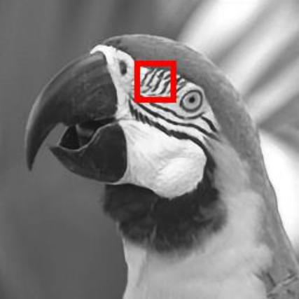
The training dataset in our experiment consists of 89,600 image patches of size , where all these patches are the luminance components randomly cropped from images in BSD500 training and testing set ( images) [3]. Each image patch consists of 9 non-overlapping blocks of size , where each block can be sampled independently by . We use Set11 for testing. For comparison, we also test four recent methods in this experiment: CS-Net [63], SCS-Net [62], BCS-Net [87] and AMP-Net [85]. All the compared methods are applied to Set11, and the average PSNR are shown in Table 2. Table 2 also shows the number of learnable parameters of the reconstruction network part of each method. In addition to these parameters, all methods also need to learn the sampling matrix with variables when and another variables of for initialization, except that BCS-Net requires over 2.2M parameters for sampling and initialization. BCS-Net learns a set of sampling matrices with different rates and dynamically assigns the sampling resource depending on the embedded saliency information of each block [87]. From Table 1, we can see that LDA outperforms all these state-of-the-art methods by a large margin, but only needs a fraction of the amount of learnable parameters compared to most methods. In Figures 2–4, we show the reconstructed butterfly and cameraman images with CS ratio as well as the parrot image with CS ratio . It is remarkable that the proposed LDA is able to recover fine patterns and details in the images, such as the texture of butterfly wing and the parrot feather shown in Figures 2 and 4, and the boundary of the camera stand in Figure 3.




4.2.3 Magnetic resonance image reconstruction
In this experiment, we consider the reconstruction problem in compressed sensing magnetic resonance imaging (CS-MRI). In CS-MRI, we set , where is a binary selection matrix representing the Fourier space (-space) sampling trajectory, and is the discrete Fourier transform. The ground truth image is shown in Figure 5(a). We use radial mask with three different sampling ratios , and in this experiments. The one with 10% sampling ratio is shown in Figure 5(a). We randomly select 2D images from the brain MRI datasets [7], then extract the main center region of interests (size ) of every image as the ground truth images , and set the data to . Then we randomly select images for training and use the other for testing.
During the training, for each of the sampling ratios 10%, 20%, and 30%, we train LDA for phase numbers , and the PSNR obtained for each case is shown in the left panel of Figure 7. For comparison, we also apply Zero-filling [8], ADMM-Net [66], ISTA-Net+ [81] and Variational Network (VN) [35] to the same data. We use as the initial for ADMM-Net, ISTA-Net+ and LDA, whereas VN takes the result of zero-filling as initial. The quantitative comparison results are shown in Table 3, where the PSNR, the relative error (RelErr) of the reconstruction to the ground truth defined by , and the structural similarity index (SSIM) [70] are provided for each of the three sampling ratios. These results show that LDA generates more accurate images using relatively much fewer network parameters. Figure 5 shows the reconstructed images obtained by ADMM-Net, ISTA-Net+, VN and LDA under sampling ratio 10%, as well as the corresponding pointwise absolute error where brighter pixels indicate larger errors. From Figure 5, it can be seen that LDA attains much lower error and better reconstruction quality.
| Method | 10% | 20% | 30% | #Par | ||||||
|---|---|---|---|---|---|---|---|---|---|---|
| PSNR | RelErr | SSIM | PSNR | RelErr | SSIM | PSNR | RelErr | SSIM | ||
| Zero-filling [8] | 23.45 | 0.2820 | 0.4544 | 27.46 | 0.1806 | 0.5820 | 30.91 | 0.1232 | 0.6665 | NA |
| ADMM-Net [66] | 30.43 | 0.1193 | 0.7990 | 37.73 | 0.0516 | 0.9507 | 41.90 | 0.0321 | 0.9646 | 14,600 |
| ISTA-Net+ [81] | 32.62 | 0.0950 | 0.9312 | 39.84 | 0.0430 | 0.9816 | 43.53 | 0.0295 | 0.9892 | 823,692 |
| VN [35] | 33.21 | 0.0882 | 0.9395 | 40.11 | 0.0400 | 0.9855 | 44.27 | 0.0249 | 0.9928 | 131,050 |
| LDA | 34.20 | 0.0790 | 0.9462 | 41.03 | 0.0363 | 0.9852 | 46.12 | 0.0214 | 0.9931 | 55,895 |


4.3 Experimental results on convergence, parameters and learned feature map
4.3.1 Comparison with standard gradient descent
The proposed LDA performs two residual-type updates, one on the data fidelity and the other on the regularization (and the smoothed version ), which is motivated by the effectiveness of the ResNet structure. In this experiment, we also unroll the standard gradient descent iteration by turning off the step of LDA, and an accelerated inertial version by setting where is also learned. We call these two networks GD-Net and AGD-Net, respectively. We test all three methods following the same experiment setting in Section 4.2.1, and show the average PSNR versus phase (iteration) number of these methods in Figure 7. As we can see, LDA achieves a much higher PNSR than both GD-Net and AGD-Net, where the latter perform very similarly. In particular, although AGD has improved iteration complexity in the standard convex optimization setting, its network version does not seem to inherit the effectiveness for deep learning applications. Similar comparison has been made for ISTA-Net and FISTA-Net, which are based on ISTA and FISTA with the latter algorithm provably having improved iteration complexity, but their deep network versions have nearly identical performance [84]. This is also partly due to the nonconvexity of the learned objective function, for which inertial gradient descent may produce improper extrapolation and do not improve efficiency.
4.3.2 Trade-offs between network performance and complexity
The regularization term of LDA is learned from training samples, yet there are still a few key network hyperparameters that have to be set manually. Specifically, we investigate the effects of several main factors of the network architecture, including the number of convolutions () and the depth of the convolution kernels (). We set the default value as and , and test the performance by varying one of them while keeping the other one as default. For fair comparison, we keep the phase number for each experiment in this study. The experiment setting and datasets are identical to Section 4.2.1, and all following results are trained and tested with CS ratio .
We first consider the effect of . We evaluate the instances of and respectively. The results are listed and compared in Table 4. As expected, the PSNR improves with larger and increased representation power, but the margin gradually decreases. On the contrary, the number of parameters and running time grow significantly in the meantime. It seems that is a good compromise between network complexity and reconstruction quality, which is also the value we used in LDA in this work.
Next we consider the effect of . We evaluate the cases of different number of convolutions and . The corresponding tested results are reported in Table 5. Again the PSNR increases with larger . However PSNR only improves slightly when increases from to , whereas the parameter number and the testing time also increase significantly. Therefore of LDA appears to be a good balance, which is the value we set for LDA in our other tests.


| Depth of conv. kernels | 8 | 16 | 32 | 48 |
|---|---|---|---|---|
| PSNR (dB) | 25.60 | 26.36 | 26.79 | 26.88 |
| Number of parameters | 1,815 | 7,071 | 27,951 | 62,655 |
| Average testing time (s) | 0.035 | 0.059 | 0.106 | 0.171 |
| Number of convolutions | 2 | 4 | 6 |
|---|---|---|---|
| PSNR (dB) | 25.83 | 26.79 | 26.95 |
| Number of parameters | 9,519 | 27,951 | 46,383 |
| Average testing time (s) | 0.058 | 0.106 | 0.164 |
4.3.3 Convergence behavior of LDA
As in the standard approach of deep neural network training, we set the phase (iteration) number to in LDA in the experiments above. On the other hand, we proved that the iterates generated by LDA converge to a Clarke stationary point in Section 3.3. This provides a theoretical guarantee that the LDA is indeed minimizing an objective function where the regularization is learned, and LDA is expected to perform stably even beyond the trained phases. To demonstrate this stability empirically, we set , and in LDA and let it continue to run after the initial 15 iterations (we use trained parameters in the first 15 iterations) on the test image House in Set11. We set which is obtained after learning. LDA automatically reduces and computes the step sizes using the standard line search backtracking with step size reduction rate such that with set to . Under this setting, the termination criterion in Step 8 of Algorithm 1 is met when total iterations and is reduced times. The changes of objective function value and PSNR in iteration number are shown in Figure 7. The objective function value versus iteration is shown in the left panel of Figure 7 and the corresponding PSNR is shown in the right panel. As we can see, LDA continues to reduce function value during these extended iterations, as shown in our convergence analysis in Section 3.3. The PSNR slightly drops after the trained 15 iterations and remains steady since after iterations. The reconstructed images during the iterations seem to be very similar without any visual artifacts despite of the slight drop of PSNR. In Figure 8, we show the reconstructed images obtained after , , , and iterations, which appear to be very similar without any visual artifacts.
4.3.4 Learned feature map in LDA
A main advantage of LDA is that the feature map in the regularization can be learned adaptively from the training data such that the network is more interpretable. This data-driven approach yields automated design of feature maps which are often more complex and efficient, rather than the manually crafted features in the classical image reconstruction models.
In this experiment, we plot the norm of the gradient (as a 2D vector computed by forward finite difference) at every pixel which is used as the feature of the TV based image reconstruction and also at pixel of the regularization learned in LDA in Figure 9. We can see that the learned feature map captures more important structural details of the images, such as the antennae of the butterfly, the buildings behind the cameraman, and the bill of the parrot. These details are crucial in species detection and facial recognition, which seem to be accurately recovered using the learned feature map but are heavily blurred or completely missing from the simple gradient image used in TV regularization. This also explains the better image quality obtained by LDA compared to the classical TV based image reconstruction methods.


5 Conclusion
We proposed a general learning based framework for solving nonsmooth and nonconvex image reconstruction problems, where the regularization function is modeled as the composition of the norm and a smooth but nonconvex feature mapping parametrized as a deep convolutional neural network. We developed a descent-type algorithm to solve the nonsmooth nonconvex minimization problem by leveraging Nesterov’s smoothing technique and the idea of residual learning, and learn the network parameters such that the outputs of the algorithm match the references in training data. Our method is versatile as one can employ various modern network structures into the regularization, and the resulting network inherits the guaranteed convergence of the algorithm. The proposed network is applied to a variety of real-world image reconstruction problems, and the numerical results demonstrate the outstanding performance and efficiency of our method.
Acknowledgments
This research was partially supported by NSF grants DMS-1319050, DMS-1719932, DMS-1818886, DMS-1925263, CMMI-2016571 and University of Florida AI Catalyst Grants.
References
- [1] M. Abadi, P. Barham, J. Chen, Z. Chen, et al. Tensorflow: A system for large-scale machine learning. In 12th Symposium on Operating Systems Design and Implementation (OSDI 16), pages 265–283, 2016.
- [2] J. Adler and O. Öktem. Learned primal-dual reconstruction. IEEE transactions on medical imaging, 37(6):1322–1332, 2018.
- [3] P. Arbelaez, M. Maire, C. Fowlkes, and J. Malik. Contour detection and hierarchical image segmentation. IEEE transactions on pattern analysis and machine intelligence, 33(5):898–916, 2010.
- [4] H. Attouch, J. Bolte, P. Redont, and A. Soubeyran. Alternating minimization and projection methods for nonconvex problems. arXiv preprint arXiv:0801.1780, 2008.
- [5] H. Attouch, J. Bolte, P. Redont, and A. Soubeyran. Proximal alternating minimization and projection methods for nonconvex problems: An approach based on the kurdyka-łojasiewicz inequality. Mathematics of Operations Research, 35(2):438–457, 2010.
- [6] H. Attouch, J. Bolte, and B. F. Svaiter. Convergence of descent methods for semi-algebraic and tame problems: proximal algorithms, forward–backward splitting, and regularized gauss–seidel methods. Mathematical Programming, 137(1-2):91–129, 2013.
- [7] S. W. e. Bennett Landman. 2013 Diencephalon Free Challenge. doi:10.7303/syn3270353, 2013.
- [8] M. A. Bernstein, S. B. Fain, and S. J. Riederer. Effect of windowing and zero-filled reconstruction of MRI data on spatial resolution and acquisition strategy. Journal of Magnetic Resonance Imaging: An Official Journal of the International Society for Magnetic Resonance in Medicine, 14(3):270–280, 2001.
- [9] W. Bian and X. Chen. Optimality and complexity for constrained optimization problems with nonconvex regularization. Mathematics of Operations Research, 42(4):1063–1084, 2017.
- [10] M. Borgerding, P. Schniter, and S. Rangan. AMP-inspired deep networks for sparse linear inverse problems. IEEE Transactions on Signal Processing, 65(16):4293–4308, 2017.
- [11] R. I. Boţ, E. R. Csetnek, and S. C. László. An inertial forward–backward algorithm for the minimization of the sum of two nonconvex functions. EURO Journal on Computational Optimization, 4(1):3–25, 2016.
- [12] K. Bredies, K. Kunisch, and T. Pock. Total generalized variation. SIAM Journal on Imaging Sciences, 3(3):492–526, 2010.
- [13] A. Buades, B. Coll, and J.-M. Morel. A non-local algorithm for image denoising. In CVPR 2005, volume 2, pages 60–65. IEEE, 2005.
- [14] A. Buades, B. Coll, and J.-M. Morel. Image denoising methods. A new nonlocal principle. SIAM review, 52(1):113–147, 2010.
- [15] J. R. Chang, C.-L. Li, B. Poczos, and B. V. Kumar. One network to solve them all: solving linear inverse problems using deep projection models. In 2017 ICCV, pages 5889–5898. IEEE, 2017.
- [16] X. Chen. Smoothing methods for nonsmooth, nonconvex minimization. Mathematical programming, 134(1):71–99, 2012.
- [17] X. Chen, J. Liu, Z. Wang, and W. Yin. Theoretical linear convergence of unfolded ista and its practical weights and thresholds. In NIPS, pages 9061–9071, 2018.
- [18] F. H. Clarke. Optimization and nonsmooth analysis, volume 5. SIAM, 1990.
- [19] G. de Carvalho Bento, S. D. B. Bitar, J. X. da Cruz Neto, A. Soubeyran, and J. C. de Oliveira Souza. A proximal point method for difference of convex functions in multi-objective optimization with application to group dynamic problems. Computational Optimization and Applications, 75(1):263–290, 2020.
- [20] K. Q. Dinh, H. J. Shim, and B. Jeon. Measurement coding for compressive imaging using a structural measuremnet matrix. In 2013 IEEE International Conference on Image Processing, pages 10–13. IEEE, 2013.
- [21] T. P. Dinh and H. A. Le Thi. Recent advances in DC programming and DCA. In Transactions on computational intelligence XIII, pages 1–37. Springer, 2014.
- [22] C. Dong, C. C. Loy, K. He, and X. Tang. Learning a deep convolutional network for image super-resolution. In ECCV, 2014.
- [23] D. Drusvyatskiy and A. S. Lewis. Error bounds, quadratic growth, and linear convergence of proximal methods. Mathematics of Operations Research, 43(3):919–948, 2018.
- [24] H. Du and Y. Liu. Minmax-concave total variation denoising. Signal, Image and Video Processing, 12(6):1027–1034, 2018.
- [25] V. Dumoulin and F. Visin. A guide to convolution arithmetic for deep learning. arXiv preprint arXiv:1603.07285, 2016.
- [26] A. Effland, E. Kobler, K. Kunisch, and T. Pock. Variational networks: An optimal control approach to early stopping variational methods for image restoration. Journal of Mathematical Imaging and Vision, pages 1–21, 2020.
- [27] J. E. Fowler, S. Mun, and E. W. Tramel. Block-based compressed sensing of images and video. Foundations and Trends in Signal Processing, 4(4):297–416, 2012.
- [28] P. Frankel, G. Garrigos, and J. Peypouquet. Splitting methods with variable metric for kurdyka–łojasiewicz functions and general convergence rates. Journal of Optimization Theory and Applications, 165(3):874–900, 2015.
- [29] M. Fukushima and H. Mine. A generalized proximal point algorithm for certain non-convex minimization problems. International Journal of Systems Science, 12(8):989–1000, 1981.
- [30] L. Gan. Block compressed sensing of natural images. In 2007 15th International conference on digital signal processing, pages 403–406. IEEE, 2007.
- [31] D. Gilton, G. Ongie, and R. Willett. Learned patch-based regularization for inverse problems in imaging. In 2019 IEEE 8th International Workshop on Computational Advances in Multi-Sensor Adaptive Processing (CAMSAP), pages 211–215. IEEE, 2019.
- [32] P. Gong, C. Zhang, Z. Lu, J. Huang, and J. Ye. A general iterative shrinkage and thresholding algorithm for non-convex regularized optimization problems. In international conference on machine learning, pages 37–45, 2013.
- [33] S. Gratton, E. Simon, and P. L. Toint. Minimization of nonsmooth nonconvex functions using inexact evaluations and its worst-case complexity. arXiv preprint arXiv:1902.10406, 2019.
- [34] K. Gregor and Y. LeCun. Learning fast approximations of sparse coding. In J. Fürnkranz and T. Joachims, editors, ICML 2010, pages 399–406, Haifa, Israel, June 2010.
- [35] K. Hammernik, T. Klatzer, E. Kobler, M. P. Recht, D. K. Sodickson, T. Pock, and F. Knoll. Learning a variational network for reconstruction of accelerated MRI data. Magnetic resonance in medicine, 79(6):3055–3071, 2018.
- [36] K. He, X. Zhang, S. Ren, and J. Sun. Deep residual learning for image recognition. In CVPR, pages 770–778, 2016.
- [37] K. He, X. Zhang, S. Ren, and J. Sun. Identity mappings in deep residual networks. In European conference on computer vision, pages 630–645. Springer, 2016.
- [38] K. Hornik, M. Stinchcombe, and H. White. Multilayer feedforward networks are universal approximators. Neural networks, 2(5):359–366, 1989.
- [39] D. P. Kingma and J. Ba. Adam: A method for stochastic optimization. arXiv preprint arXiv:1412.6980, 2014.
- [40] E. Kobler, A. Effland, K. Kunisch, and T. Pock. Total deep variation for linear inverse problems. In Proceedings of the IEEE/CVF Conference on Computer Vision and Pattern Recognition, pages 7549–7558, 2020.
- [41] K. Kulkarni, S. Lohit, P. Turaga, R. Kerviche, and A. Ashok. ReconNet: Non-iterative reconstruction of images from compressively sensed measurements. In CVPR, pages 449–458, 2016.
- [42] C. Lemaréchal and C. Sagastizábal. Practical aspects of the Moreau–Yosida regularization: Theoretical preliminaries. SIAM Journal on Optimization, 7(2):367–385, 1997.
- [43] A. S. Lewis and S. J. Wright. A proximal method for composite minimization. Mathematical Programming, 158(1-2):501–546, 2016.
- [44] C. Li, W. Yin, H. Jiang, and Y. Zhang. An efficient augmented Lagrangian method with applications to total variation minimization. Computational Optimization and Applications, 56(3):507–530, 2013.
- [45] H. Li and Z. Lin. Accelerated proximal gradient methods for nonconvex programming. In Advances in neural information processing systems, pages 379–387, 2015.
- [46] H. Li, J. Schwab, S. Antholzer, and M. Haltmeier. NETT: Solving inverse problems with deep neural networks. Inverse Problems, 2020.
- [47] J. Liu, X. Chen, Z. Wang, and W. Yin. ALISTA: Analytic weights are as good as learned weights in LISTA. ICLR, 2019.
- [48] Z. Lu, H. Pu, F. Wang, Z. Hu, and L. Wang. The expressive power of neural networks: A view from the width. In NIPS, pages 6231–6239, 2017.
- [49] T. Meinhardt, M. Moller, C. Hazirbas, and D. Cremers. Learning proximal operators: Using denoising networks for regularizing inverse imaging problems. In ICCV, pages 1781–1790, 2017.
- [50] C. A. Metzler, A. Maleki, and R. G. Baraniuk. From denoising to compressed sensing. IEEE Transactions on Information Theory, 62(9):5117–5144, 2016.
- [51] R. Mifflin, L. Qi, and D. Sun. Properties of the Moreau-Yosida regularization of a piecewise C2 convex function. Mathematical programming, 84(2):269–281, 1999.
- [52] J.-J. Moreau. Proximité et dualité dans un espace hilbertien. Bulletin de la Société mathématique de France, 93:273–299, 1965.
- [53] Y. Nesterov. Smooth minimization of non-smooth functions. Mathematical programming, 103(1):127–152, 2005.
- [54] Y. Nesterov. Gradient methods for minimizing composite functions. Mathematical Programming, 140(1):125–161, 2013.
- [55] Y. E. Nesterov. A method for solving the convex programming problem with convergence rate . Dokl. Akad. Nauk SSSR, 269:543–547, 1983.
- [56] J. C. Neto, P. R. Oliveira, A. Soubeyran, and J. Souza. A generalized proximal linearized algorithm for DC functions with application to the optimal size of the firm problem. Annals of Operations Research, pages 1–27, 2018.
- [57] P. Ochs, Y. Chen, T. Brox, and T. Pock. iPiano: Inertial proximal algorithm for nonconvex optimization. SIAM Journal on Imaging Sciences, 7(2):1388–1419, 2014.
- [58] P. Ochs, A. Dosovitskiy, T. Brox, and T. Pock. On iteratively reweighted algorithms for nonsmooth nonconvex optimization in computer vision. SIAM Journal on Imaging Sciences, 8(1):331–372, 2015.
- [59] P. Ochs, J. Fadili, and T. Brox. Non-smooth non-convex bregman minimization: Unification and new algorithms. Journal of Optimization Theory and Applications, 181(1):244–278, 2019.
- [60] R. T. Rockafellar. Variational analysis, 1998.
- [61] L. I. Rudin, S. Osher, and E. Fatemi. Nonlinear total variation based noise removal algorithms. Physica D: Nonlinear Phenomena, 60(1):259–268, 1992.
- [62] W. Shi, F. Jiang, S. Liu, and D. Zhao. Scalable convolutional neural network for image compressed sensing. In The IEEE Conference on Computer Vision and Pattern Recognition (CVPR), June 2019.
- [63] W. Shi, F. Jiang, S. Zhang, and D. Zhao. Deep networks for compressed image sensing. In 2017 IEEE International Conference on Multimedia and Expo (ICME), pages 877–882. IEEE, 2017.
- [64] J. C. O. Souza, P. R. Oliveira, and A. Soubeyran. Global convergence of a proximal linearized algorithm for difference of convex functions. Optimization Letters, 10(7):1529–1539, 2016.
- [65] P. Sprechmann, A. M. Bronstein, and G. Sapiro. Learning efficient sparse and low rank models. IEEE transactions on pattern analysis and machine intelligence, 37(9):1821–1833, 2015.
- [66] J. Sun, H. Li, Z. Xu, et al. Deep ADMM-Net for compressive sensing MRI. In Advances in Neural Information Processing Systems, pages 10–18, 2016.
- [67] Y. Sun, J. Chen, Q. Liu, B. Liu, and G. Guo. Dual-path attention network for compressed sensing image reconstruction. IEEE Transactions on Image Processing, 29:9482–9495, 2020.
- [68] P. D. Tao et al. The DC (difference of convex functions) programming and DCA revisited with DC models of real world nonconvex optimization problems. Annals of operations research, 133(1-4):23–46, 2005.
- [69] S. Wang, S. Fidler, and R. Urtasun. Proximal deep structured models. In Advances in Neural Information Processing Systems, pages 865–873, 2016.
- [70] Z. Wang, A. C. Bovik, H. R. Sheikh, and E. P. Simoncelli. Image quality assessment: from error visibility to structural similarity. IEEE transactions on image processing, 13(4):600–612, 2004.
- [71] B. Wen, X. Chen, and T. K. Pong. A proximal difference-of-convex algorithm with extrapolation. Computational optimization and applications, 69(2):297–324, 2018.
- [72] S. Xie, R. Girshick, P. Dollár, Z. Tu, and K. He. Aggregated residual transformations for deep neural networks. In Proceedings of the IEEE conference on computer vision and pattern recognition, pages 1492–1500, 2017.
- [73] X. Xie, J. Wu, Z. Zhong, G. Liu, and Z. Lin. Differentiable linearized ADMM. arXiv preprint arXiv:1905.06179, 2019.
- [74] B. Xin, Y. Wang, W. Gao, D. Wipf, and B. Wang. Maximal sparsity with deep networks? In NIPS, pages 4340–4348, 2016.
- [75] H. Yao, F. Dai, S. Zhang, Y. Zhang, Q. Tian, and C. Xu. DR2-Net: Deep residual reconstruction network for image compressive sensing. Neurocomputing, 359:483–493, 2019.
- [76] D. Yarotsky. Error bounds for approximations with deep ReLU networks. Neural Networks, 94:103–114, 2017.
- [77] K. Yosida. Functional Analysis. Springer, Berlin, 1964.
- [78] S. Zagoruyko and N. Komodakis. Wide residual networks. arXiv preprint arXiv:1605.07146, 2016.
- [79] C. Zhang and X. Chen. Smoothing projected gradient method and its application to stochastic linear complementarity problems. SIAM Journal on Optimization, 20(2):627–649, 2009.
- [80] J. Zhang and B. Ghanem. Ista-net: Iterative shrinkage-thresholding algorithm inspired deep network for image compressive sensing. 2017.
- [81] J. Zhang and B. Ghanem. ISTA-Net: Interpretable optimization-inspired deep network for image compressive sensing. In CVPR, 2018.
- [82] J. Zhang, C. Zhao, and W. Gao. Optimization-inspired compact deep compressive sensing. IEEE Journal of Selected Topics in Signal Processing, 2020.
- [83] K. Zhang, W. Zuo, Y. Chen, D. Meng, and L. Zhang. Beyond a gaussian denoiser: Residual learning of deep cnn for image denoising. IEEE transactions on image processing, 26(7):3142–3155, 2017.
- [84] K. Zhang, W. Zuo, S. Gu, and L. Zhang. Learning deep CNN denoiser prior for image restoration. In CVPR, pages 3929–3938, 2017.
- [85] Z. Zhang, Y. Liu, J. Liu, F. Wen, and C. Zhu. AMP-Net: Denoising based deep unfolding for compressive image sensing. arXiv preprint arXiv:2004.10078, 2020.
- [86] W. Zhong and J. T. Kwok. Gradient descent with proximal average for nonconvex and composite regularization. In Twenty-Eighth AAAI Conference on Artificial Intelligence, 2014.
- [87] S. Zhou, Y. He, Y. Liu, and C. Li. Multi-channel deep networks for block-based image compressive sensing. arXiv preprint arXiv:1908.11221, 2019.