Fused-Lasso Regularized Cholesky Factors of Large Nonstationary Covariance Matrices of Longitudinal Data
Abstract
Smoothness of the subdiagonals of the Cholesky factor of large covariance matrices is closely related to the degrees of nonstationarity of autoregressive models for time series and longitudinal data. Heuristically, one expects for a nearly stationary covariance matrix the entries in each subdiagonal of the Cholesky factor of its inverse to be nearly the same in the sense that sum of absolute values of successive terms is small. Statistically such smoothness is achieved by regularizing each subdiagonal using fused-type lasso penalties. We rely on the standard Cholesky factor as the new parameters within a regularized normal likelihood setup which guarantees: (1) joint convexity of the likelihood function, (2) strict convexity of the likelihood function restricted to each subdiagonal even when , and (3) positive-definiteness of the estimated covariance matrix. A block coordinate descent algorithm, where each block is a subdiagonal, is proposed and its convergence is established under mild conditions. Lack of decoupling of the penalized likelihood function into a sum of functions involving individual subdiagonals gives rise to some computational challenges and advantages relative to two recent algorithms for sparse estimation of the Cholesky factor which decouple row-wise. Simulation results and real data analysis show the scope and good performance of the proposed methodology.
Keywords: Nonstationary covariance matrices, Gaussian graphical models, Cholesky factor, fused-lasso, precision matrices
MOS subject classifications: 62A09, 60G99
1 Introduction
A salient feature of stationary time series analysis is its reliance on the Cholesky decomposition to model temporal dependence and the dynamics. Important examples include moving average models (Cholesky decomposition of a covariance matrix), autoregressive (AR) models (Cholesky decomposition of an inverse covariance matrix), ARMA models in the time-domain (Ansley 1979), see Dai and Guo 2004; Rosen and Stoffer 2007 for explicit use of the Cholesky factors in the spectral-domain. For nonstationary time series the focus has been on (time-)varying coefficients AR models (Gabriel 1962; Rao 1970; Kitagawa and Gersch 1985; Dahlhaus 1997; Zimmerman and Nunez-Anton 2010).
Recently, a similar dichotomy is taking roots in the modern multivariate statistics and machine learning where the focus is on either estimation of large covariance or inverse covariance matrices of longitudinal data using Cholesky decomposition. Whereas the entries of a covariance matrix quantifies pairwise or marginal dependence, those of the precision or inverse covariance matrix specifies multivariate relationships among the variables in a -dimensional random vector with a positive-definite covariance matrix . More precisely, when follows a Gaussian distribution a zero off-diagonal entry of or implies that and are conditionally independent given all other variables (Whittaker 1990). When the number of observations is less than the number of variables , it is reasonable to impose structure or regularize directly in the search for sparsity (Banerjee et al. 2008; Friedman et al. 2008), see Pourahmadi 2013 for an overview.
The use of the modified Cholesky decomposition of was advocated in (Pourahmadi 1999; Wu and Pourahmadi 2003), Huang et al. 2006 and Levina et al. 2008 for parsimony (GLM-based) and sparse (regularized) estimation of its Cholesky factor and hence the precision matrix. Recall that the standard and modified Cholesky factors of a positive-definite precision matrix are defined and connected by
| (1) |
where is a unique lower triangular matrix with positive diagonal entries and is a unit lower triangular matrix with diagonal entries equal to 1, is a diagonal matrix with positive diagonal entries. For time series and longitudinal data the entries in each row of have the useful interpretation as the regression coefficients and each diagonal entry of as the variance of the residual of regressing a variable on its preceding variables:
| (2) |
The genesis of this representation and interpretation of the coefficients for stationary processes can be traced to the rise of finite-parameter AR models in 1920’s (Pourahmadi 2001, Section 1.2); (Ansley 1979). For example, a stationary AR model of order is closely related to a -banded lower triangular matrix where all entries of its first subdiagonal are the same and equal to the negative of the lag-1 AR coefficient, and so on. Heuristically, one expects for a nearly stationary (Toeplitz) covariance matrix the entries in each subdiagonal of the Cholesky factor of the inverse covariance matrix to be nearly the same in the sense that sum of absolute values of its successive terms is small. Important examples of mild departures from stationarity are locally stationary (Dahlhaus 1997) and piecewise stationary (Adak 1998; Davis et al. 2006) processes where in the latter the subdiagonals could be certain step functions. Figure 10 illustrates the adverse effect of learning a genuinely nonstationary covariance matrix of the cattle data (Kenward 1987) using a (misspecified) stationary AR model.
We emphasize the time-varying nature of the coefficients in (2) for fixed by using a doubly indexed triangular array (Dahlhaus 1997) and writing it more generally as
| (3) |
where , ) and are smooth functions of the rescaled time and ’s are i.i.d. random variables with mean zero and variance one. This rescaling enables one to view the (sub)diagonals of and as realizations of smooth functions (see Figure 1) and brings the estimation problem within the familiar nonparametric infill asymptotic setup where one observes the smooth functions ) and on a finer grids for a larger . Interestingly, choosing ) and as functions of bounded variation guarantees that, under mild conditions, the solutions of (3) are locally stationary processes (Dahlhaus and Polonik 2009, Proposition 2.4).
In addition to its profound conceptual impact on time series analysis (Dahlhaus 2012), the functional view of (3) for longitudinal data has been a major source of inspiration for nonparametric estimation of the subdiagonals of , see Wu and Pourahmadi 2003 and Huang et al. 2007. Furthermore, within the smoothing spline ANOVA framework, Blake 2018 treats the AR coefficients as a bivariate smooth function and decomposes it in the stationary direction of the lag and the nonstationary (additive) direction and a possible interaction term. Then, regularizing the nonstationary direction more heavily amounts to shrinking the covariance estimator toward the more parsimonious and desirable stationary structures.
In the longitudinal data setup, with a sample and the sample covariance matrix , its log-likelihood function was used for penalized likelihood estimation of the parameters in Huang et al. 2006, see also Levina et al. 2008 and Khare et al. 2019 for a comprehensive review. The lack of convexity of the likelihood in was noted first in Khare et al. 2019 and Yu and Bien 2017. They ensure convexity by reparameterizing the likelihood in terms of the standard Cholesky factor rather than the customary -parametrization. While the last identity in (1) reveals that and share the same sparsity patterns, the connection between the degree of smoothness of their subdiagonals is a bit more complicated and controlled by the boundedness and smoothness of the diagonal entries of (see Lemma 5).
This paper is concerned with smoothness through regularizing the subdiagonals of the Cholesky factor of using the fused Lasso penalties (Tibshirani et al. 2005) as an alternative to their smooth (nonparametric) estimation. More specifically, using the family of fused lasso penalty functions on the subdiagonals we propose a novel smooth Cholesky (SC) algorithm for estimating the subdiagonals of and hence the (inverse) covariance matrix via a block coordinate decent algorithm. The SC objective function is convex in , and compared to the recent algorithms in Khare et al. 2019 and Yu and Bien 2017 when , the update of each block is obtained by solving a strictly convex optimization problem. We establish the convergence of the iterates to stationary points of the objective function, and elaborate on the connection between the smoothness of the subdiagonals of and those of under the assumption of boundedness of the diagonal entries of .
The remainder of the paper is organized as follows. Section 2 introduces the SC algorithm and studies its convergence and computational complexity. Section 3 establishes the connection between smoothness of subdiagonals of and . Section 4 illustrates the performance of the SC methodology through simulations and real data analysis, and demonstrates its ability to model and detect the smoothness of the subdiagonals of Cholesky factor. Consequently, estimation of the covariance matrix and its role in forecasting the future calls in a call center are investigated. Appendices contain proofs of the result in the paper and some additional simulations. All appendices are placed in Supporting Information.
Our SC algorithm and the corresponding methodology for longitudinal data can be specialized to the setup of a long stretch of a single stationary time series, namely for and large. To this end, banded estimates of Toeplitz covariance matrices and properties of the corresponding optimal linear predictors are studied in Wu and Pourahmadi 2009; Bickel and Gel 2011 and McMurry and Politis 2010; McMurry and Politis 2015. For covariance estimation and prediction of locally stationary processes, see Das and Politis 2020.
In the rest of this section, we introduce notation used throughout the paper. For a vector , we define its norm for . We denote by the space of all lower triangular matrices with positive diagonal elements. Given a lower-triangular matrix , the vector is its standard vectorization formed by stacking up its column vectors including the zero (redundant) entries. Each vector of (sub)diagonal entries of corresponds to those from with the following set of indices:
so that corresponds to the main diagonal entries, is the -subvector of the th subdiagonal entries. We denote by a vector of diagonal and subdiagonals, except for the th subdiagonal. For simplicity in notation, we replace by so that for a given matrix and index sets , denotes the submatrix with column indices selected from , and is the submatrix with rows and columns of indexed by and , respectively.
2 The Smooth Cholesky Algorithm
In this section, we develop the SC algorithm for a convex penalized likelihood function using fused-type Lasso penalties on the subdiagonals of the standard Cholesky factor. Such penalties are bound to induce various degrees of sparsity and smoothness on the subdiagonals, but our main focus is on smoothness. The objective functions turn out to be conditionally separable. Computational and statistical properties of a block coordinate descent algorithm for its minimization are studied.
2.1 The Gaussian-Likelihood and Fused Lasso Penalties
Let be the Gaussian log-likelihood function for a sample of size from a zero-mean normal distribution with the precision matrix . Its convexity is ensured by reparametrizing it in terms of the standard Cholesky factor , see Khare et al. 2019 and Yu and Bien 2017. More precisely, we consider
| (4) |
where is a convex penalty function. There are two recent important choices of designed to induce sparsity in the rows of the Cholesky factor.
The method of Convex Sparse Cholesky Selection (CSCS) of in Khare et al. 2019 employs the penalty . The ensuing objective function turns out to be jointly convex in the (nonredundant) entries of , bounded away from even if ; but it is not strictly convex in the high-dimensional case. A cyclic coordinatewise minimization algorithm is developed in Khare et al. 2019 to compute . Note that once is computed using the CSCS or other methods considered here, then one can compute , the (inverse) covariance matrix and . Sparsity of is not guaranteed since the sparsity pattern of the estimated in Khare et al. 2019, as in Huang et al. 2006 and Shojaie and Michailidis 2010, has no particular structure. Fortunately, a more structured sparse which guarantees sparsity of the precision matrix is developed in Yu and Bien 2017. Their hierarchical sparse Cholesky (HSC) method relies on the hierarchical group penalty where the ’s are quadratically decaying weights. The HSC method has the goal of learning the local dependence among the variables and leads to a more structured sparsity with a contiguous stretch of zeros in each row away from the main diagonal. Its flexibility is similar to that of the nested lasso in Rothman et al. 2010. Yu and Bien 2017 relies on an alternating direction method of multipliers (ADMM) approach to compute . Computationally, both penalty functions lead to a decoupling of the above objective function into separate and parallelizable optimization problems each involving a separate row of .
For the SC algorithm developed in this paper, we employ a number of fused lasso penalty functions on the Cholesky factor or its subdiagonals. However, unless stated otherwise the phrase fused lasso refers to
based on the -norm of the first differences. Note that this is slightly different from the more general sparse fused lasso penalty function in Tibshirani et al. 2005 and Tibshirani and Taylor 2011 which is of the form
The latter includes an additional lasso penalty term to achieve sparsity on top of smoothness of the subdiagonals. Note that our usage of fused lasso is more in the spirit of the total variation penalty in Rudin et al. 1992.
When higher-order smoothness of the subdiagonals is desirable, then it is natural to penalize sum of higher-order differences such as , the -trend filtering (Kim et al. 2009), and (Hodrick and Prescott 1997), referred to as H-P hereafter, where is the matrix of second-order differences:
For other higher order difference matrices belonging to the family of generalized lasso penalties, see Tibshirani et al. 2005;Tibshirani and Taylor 2011.
2.2 The Conditionally Separable Convex Objective Function
We express the objective function (4) as the sum of quadratic functions each involving distinct (sub)diagonals of (given the others), so that it is conditionally separable. This is in sharp contrast to the objective functions in Khare et al. 2019 and Yu and Bien 2017 which decouple over the rows of the matrix with nice computational consequences. Nevertheless, our objective function is jointly convex in , and strictly convex when .
Let be the Kronecker product of the sample covariance matrix from a sample of size and the identity matrix. The structure of the matrix and the submatrices , introduced in the proof of the following Lemma play a vital role in proving properties of our SC algorithm.
Lemma 1.
For the lower triangular matrix it holds that:
- (a)
The first term in (4) can be rewritten as
(5) - (b)
The objective function is conditionally separable in that
(6) where for and fixed ,
(7) and
(8) - (c)
’s are strictly convex in even when .
A proof of the lemma is provided in the Appendix. Parts (a) and (b) are fundamental for constructing our SC algorithm in the spirit of the coordinate descent algorithm in Khare et al. 2019. However, since our objective function is not separable over the subdiagonals, the details of the proof of our block coordinate descend algorithm differ considerably from those in Khare et al. 2019.
2.3 A Block Coordinate Descent Algorithm
In this section, relying on the conditional separability as expressed in (6) we minimize using a block coordinate descent algorithm where each block corresponds to a subdiagonal of given the values of the others. The minimization of is done sequentially over the summands , . In this sense, our SC algorithm is different from the recent approaches in covariance estimation where the objective functions are either minimized by iterating over the columns of a covariance matrix (Banerjee et al. 2008; Friedman et al. 2008) or the rows of its Cholesky factor (Khare et al. 2019; Yu and Bien 2017). However, it inherits some of the desirable convergence properties of the latter two algorithms even though their optimization problems decouples into parallel problems over the rows of the matrix .
The following two generic functions stand for the objective function restricted to each (sub)diagonal:
| (9) |
and
| (10) |
where is a diagonal matrix introduced in Lemma 1, and is a vector. Note that the function is from to and is from to for . These functions are simpler than those in Khare et al. 2019 since the matrices are diagonal with positive diagonal entries so that for a fixed vector , ’s are strictly convex functions (Lemma 1). We note that a block coordinate descent algorithm which sequentially optimizes with respect to each will also optimize the objective function .
Consider the global minimizers of and :
| (11) |
Next, we show that the vector has a closed-form and provide methods to compute for various members of the fused-type Lasso family.
Lemma 2.
- (a)
For a given , is unique and its entries have the closed-form:
(12) - (b)
For a given (), corresponds to the unique solution of the fused lasso problem (Tibshirani and Taylor 2011, Algorithm 1) for the th subdiagonal of .
- (c)
When in (10) is the matrix of second-order differences, then
- (1)
corresponds to the solution of the -trend filtering (Kim et al. 2009, Section 6).
- (2)
For , has a closed form and corresponds to the H-P solution:
- (1)
- (d)
A proof of the lemma is provided in the Appendix. It provides the necessary ingredients for minimizing the objective function (6) via the following block coordinate descent algorithm where each block is a (sub)diagonal of the standard Cholesky factor .
We note that the Algorithm 1 is well-defined so long as the diagonal entries of sample covariance matrix and the initial Cholesky factor are positive. That is the minimum in the optimization appearing in line 8 of the algorithm is attained. This follows from Part (b) of Theorem 1 and the fact that ’s are strictly convex functions of .
2.4 Convergence of the SC Algorithm
In this section, we establish convergence of the SC algorithm under the weak restriction that the diagonal entries of are positive.
A key step is to reduce the objective function (6) to the following widely used objective function in the statistics and machine learning communities (Khare and Rajaratnam 2014):
| (14) |
where is a tuning parameter, is a given subset of indices and the matrix does not have a zero column. Since the objective function restricted to each subdiagonal (line 8 in Algorithm 1) is strictly convex, a unique global minimum with respect to each subdiagonal is guaranteed even when . This additional strict convexity property along with Theorems 2.1 and 2.2 in Khare and Rajaratnam 2014 are the key ingredients for showing that the iterates in SC algorithm converge to the global minimum of the objective function .
Theorem 1.
- (a)
The objective function with the fused Lasso penalty admits the generic form:
(15) where,
and the set of indices consists of the last element of and along with those of difference forms, and is a suitable matrix with no columns.
- (b)
If , then the sequence of iterates in Algorithm 1 converges to a global minimum of .
Proof of the theorem given in the Appendix relies on the following:
Lemma 3.
For every and
where is a vector of 1’s and is a positive semi-definite matrix. Moreover, any global minimizer of over the open set lies in .
A discussion of convergence of the sequence of iterates for -trend filtering and HP is provided in the Appendix E.
2.5 Computational Complexity of the SC Algorithm
The sequential SC algorithm in each iteration sweeps over the diagonal and subdiagonals of where in each sweep it must compute and . For example, for fused lasso penalty, from Lemma 1, updating each subdiagonal requires solving a fused lasso problem. Therefore, the computational cost of each subdiagonal update depends on the chosen penalty function. Denoting by the computational cost for the chosen penalty to minimize , the next lemma provides the computational cost for each iteration of SC algorithm.
Lemma 4.
The computational cost of Algorithm 1 in each iteration is .
The proof is provided in Appendix F. For example, for for the -trend filtering penalty (Kim et al. 2009). Thus, the computational cost of the SC algorithm is which is comparable to the cost of the existing sequential algorithms such as GLasso (Friedman et al. 2008), SPACE (Peng et al. 2009) and CONCORD (Khare et al. 2015) and CSCS (Khare et al. 2019) when iterations have been run sequentially.
3 Connections Among , and Local Stationarity
A key feature of our SC algorithm is its ability to capture the smoothness of subdiagonals of the Cholesky factors through regularized likelihood estimation rather than the traditional (non)parameteric methods. In this section, we explore the connection between smoothness of and when the diagonal elements of are bounded away from zero.
Smoothness of time-varying covariance and spectral density functions (Dahlhaus 1997) and subdiagonals of are usually studied by embedding the underlying nonstationary process in a doubly indexed sequence (triangular arrays), and functions defined on the rescaled time . For example, Figure 1 provides a simple illustration of the correspondence between the time-varying AR(1) model in (3), with , and the subdiagonals of .
The next lemma connects the smoothness of the entries of the th subdiagonal of the Cholesky factors and the diagonal entries of the matrix viewed as functions on . More precisely, the th subdiagonal and other matrices is viewed as a function of time by writing: where stands for its th element. In this section, smoothness of a function refers to the function being of bounded total variation where the total variation (TV) of a function is defined as
for ’s of the form .
Lemma 5.
(a) If , then for any of the form , we have
(b) If in addition, and the th subdiagonal are functions of bounded total variation on the rescaled interval with , , and , then is of bounded total variation and
| (16) |
The proof of the lemma is provided in the Appendix G.
The requirement of being of bounded variation on and open up a window to connect and extend the class of time-varying AR models to locally stationary processes. In particular, a process (t=1,…,N) with a time-varying MA()-representation: is locally stationary (Dahlhaus 1997; Dahlhaus and Polonik 2009; Dahlhaus 2012) if
| (17) |
where ’s are such that there exists functions satisfying
for a constant and and otherwise. It follows from (17) that the time-varying spectral density and the lag- covariance at the rescaled time are of the form
where
The time-varying AR models in (3) can be enlarged to the class of locally stationary time-varying ARMA models (Dahlhaus and Polonik 2009, Proposition 2.4) by choosing its coefficients and the variance functions to be of bounded variation. More precisely, if all the coefficients , and the variance functions are of bounded variation, then under usual conditions on the roots of the characteristic polynomials, the system of difference equations
| (18) |
has a locally stationary solution of the form (17).
A related topic of interest is the connections between smoothness of the standard Cholesky factor and the covariance matrix of nonstationary processes. Interestingly, it is known (Chern and Dieci 2000, Lemma 2.8) that smoothness of a covariance (positive-definite matrix-valued) function is inherited by its unique standard Cholesky factor when smoothness is in terms of degree of differentiability. Furthermore, it is known (Dahlhaus and Polonik 2009, Proposition 5.4) that the subdiagonals of covariance matrices of locally stationary processes are functions of bounded variation. Next, we establish the connection (equivalence) between the subdiagonals of the standard Cholesky factor and a covariance matrix being of bounded variation.
Proposition 1.
- (a)
If the (sub)diagonals of the Cholesky factor are of bounded variation on the rescaled interval with , then the (sub)diagonals of the matrix are of bounded variation with
- •
(b) The converse of (a) is true.
The proof is relegated to the Appendix.
4 Simulation and Data Analysis
In this section, we illustrate and gauge the performance of our methodology using simulated and real datasets. We use three commonly used penalty functions: fused lasso, -trend filtering and Hodrick-Prescott (H-P) filtering (Hodrick and Prescott 1997), and the corresponding SC algorithm is referred to as SC-Fused, SC-Trend and SC- HP, respectively.
4.1 The Simulation Setup: Four Cases of T
In all simulations, the sample sizes are , and dimensions , covering settings where and , respectively. Each simulated dataset is centered to zero and scaled to unit variance. The tuning parameter is chosen from the range over equally spaced grid points using the BIC and CV criterion described in the Appendix I. We repeat the simulation 20 times. As inputs to the Algorithm 1, we set the tolerance and the initial Cholesky factor is the diagonal matrix with diagonal elements equal to .
We start with a pair and use the parameterization as in (Khare et al. 2019) where is a diagonal matrix and is a unit lower-triangular matrix constructed for the four cases A-D described below. For given pairs , sample data are drawn independently from . In each case, except for the Case B, where the number of nonzero subdiagonals is equal 2, the number of non-zero subdiagonals is restricted to be , that is in each iteration the SC algorithm sweeps only over the first 5 subdiagonals and the rest of subdiagonals are set to 0. Except for the Cases A and B, construction of the matrix starts with generating its first subdiagonal, and then filling the rest of its subdiagonals by eliminating the last element of the previous subdiagonal. The diagonal elements of , for the Cases A and B are equal one and are of the form for the Cases C and D.
The four cases of with varying degrees of smoothness (nonstationarity) of their subdiagonals and the diagonal matrix considered are:
- Case A:
A stationary AR(1) model where is a Toeplitz matrix with the value for the first subdiagonal randomly chosen from the uniform distribution on .
- Case B:
Resembles an AR(2) model as in Davis et al. 2006 dealing with piecewise stationary processes:
where . The matrix here is 2-banded and the diagonal elements of are equal to 1 (See Figure 2).
- Case C:
The first subdiagonal of is given by , , corresponding to a (time) varying-coefficient AR model (Wu and Pourahmadi 2003).
- Case D:
The first subdiagonal of is generated according to
with and is a simple Markov process (Kim et al. 2009, Section 4). That is with probability m, and with probability it is chosen from the uniform distribution where
Figure 2 illustrates plots of the first subdiagonal of the matrix versus the rescaled time in for the four cases with .

4.2 Capturing Smoothness: A Graphical Comparison
First, we assess graphically the ability of our methodology to learn the varying degrees of smoothness of the first subdiagonal for the four cases introduced above. Figures 3 and 4 illustrate the simulation results using the SC algorithm for and , respectively. In each 2 by 4 layout, each column corresponds to one of the four cases and the row to the criteria (BIC or CV) for choosing the tuning parameters. The results for and were similar, therefore we report only those for the larger sample size.
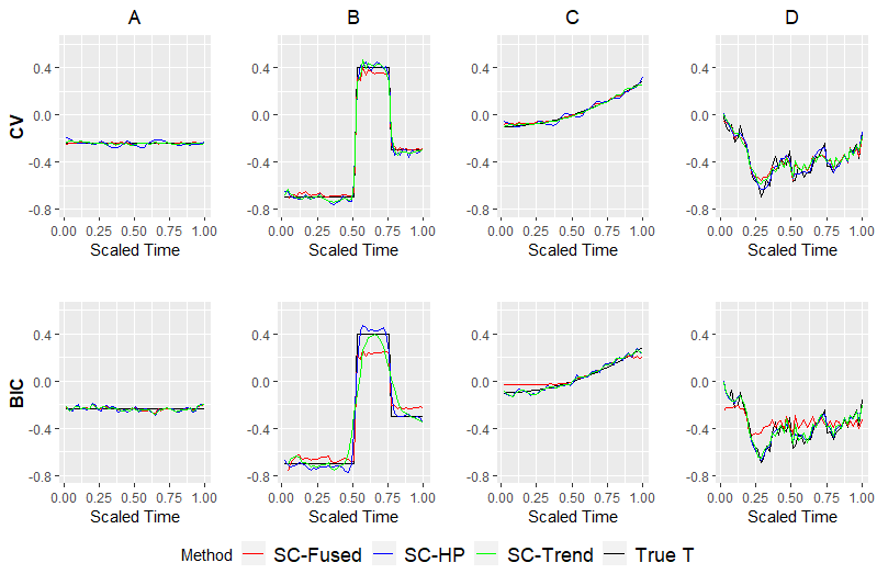

The simulation results in both figures provide ample evidence on the good performance of the SC method for estimating time-varying subdiagonals. In particular, for the Case A, as expected, the SC-Fused learns perfectly the flatness (stationarity) of the first subdiagonal, showing only some wiggliness for the BIC. For the Case B, which corresponds to a piecewise stationary process, estimators tuned using CV and BIC correctly identify the jumps and show small oscillation around the flat segments. The CV criterion shows an advantage over the BIC for the Case C. More specifically, the SC-Trend learns better the quadratic structure of the first subdiagonal than the other estimators. For the case D the SC-Trend and SC-HP provide nearly identical estimates of the first subdiagonal. The results for the other subdiagonals nearly match those in Figures 3 and 4, and are omitted. As gets larger, there seems to be evidence of improvement in performance of the SC algorithm.
4.3 Comparing Estimation Accuracies
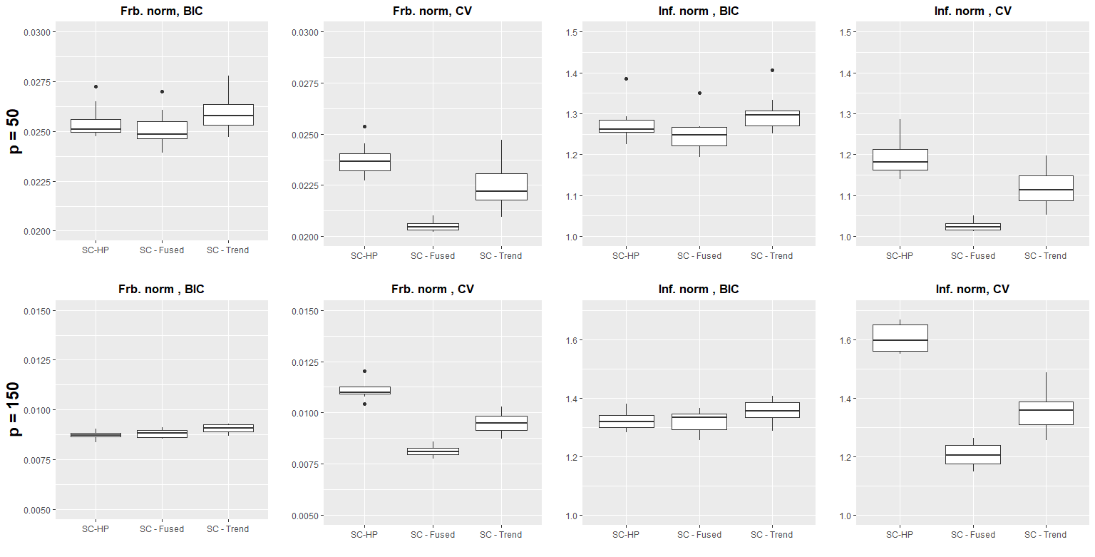
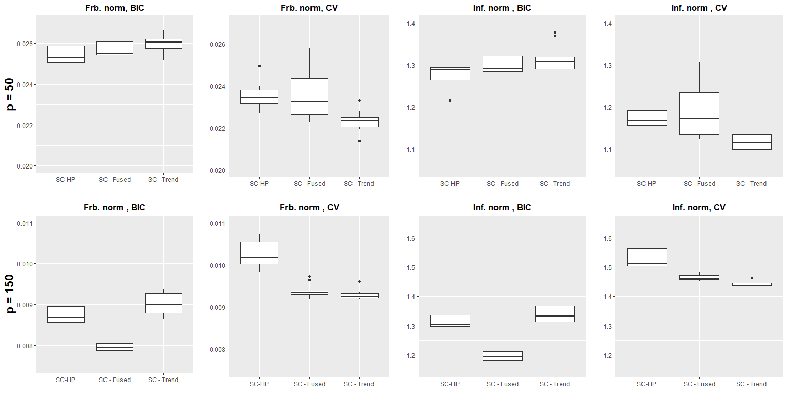
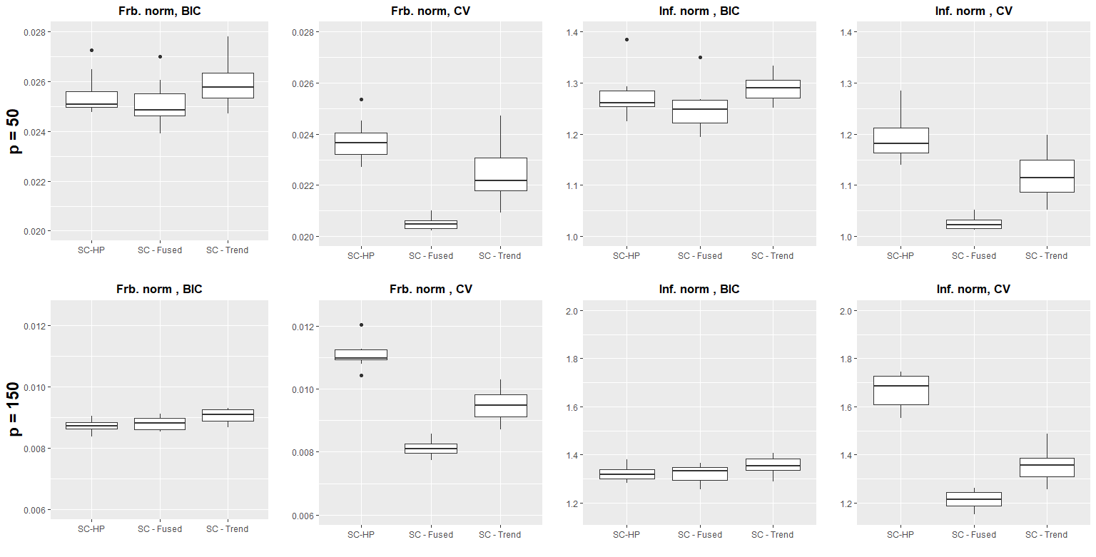
In this section, we compare the accuracies of the three SC estimators: SC-HP, SC-Fused and SC-Trend. The overall measures of performance involve magnitudes of the estimation errors and , as measured by the scaled Frobenius norm , and the matrix infinity norm for a matrix .
Boxplots of the overall estimation errors for the matrix are reported in Figures 5 through 8, where each figure corresponds to a particular case, each row to a value of and the two columns correspond to using BIC and CV criteria, respectively. They corroborate the findings in the graphical explorations Figures 3 and 4, in that the SC-Fused shows tendency to capture well cases with constant subdiagonals, SC-Trend and HP are better in capturing the wiggliness and smoothness of the subdiagonal. The corresponding estimation errors for the matrix show similar patterns, and are thus omitted.

In the Appendix J we provide two additional simulations for a more general matrix () than those in Cases A-D, and to compare our sparse SC with the existing sparse Cholesky estimators (CSCS, HSC) so far support recovery is concerned. The results confirm the good performance of the SC method. The two general matrices are: (1) is a full lower triangular matrix and its subdiagonals are chosen randomly from the Cases (A-D), (2) has a nonhierarchical structure (Yu and Bien 2017), that is nonzero subdiagonals are followed by block zero subdiagonals and again by nonzero subdiagonals.
4.4 Covariance Estimators
In this section, we assess the performance of our method on learning (inverse) covariance matrices for the Cases A-D. We compare our SC method (Fused, HP, Trend) with the CSCS and HSC methods. To make them comparable, instead of limiting the SC algorithm to run over the first five subdiagonals, as in the last two sections, here we use the more general sparse SC estimator (see Lemma 2) with the two tuning parameters and , respectively. Due to space limitation, we report results only for the with the tuning parameters selected using the CV criterion.
We evaluate performance of the estimators using the scaled Kullback-Leibler loss for the inverse covariance and scaled Frobenious norm for the covariance matrix. From results reported in Figures 9(a) and 9(b) for cases A, B, and C, it is evident that the SC algorithm learns the covariance matrix better than the SCSC and HSC methods. In particular, for the case A, SC-Fused provides the lowest error measure and for cases B and C, SC-Trend and HP are the lowest. For the Case D, the HSC is the best. For learning the inverse covariance matrix, the SC performs better for all the four cases.


4.5 The Cattle Data
This dataset Kenward 1987 is from an experiment in which cattle were assigned randomly to two treatment groups A and B. The weights of animals were recorded to study the effect of treatments on intestinal parasites. The animals were weighed times over 122 days. Of 60 cattle received treatment and the other received treatment . The dataset has been widely used in the literature of longitudinal data analysis (Wu and Pourahmadi 2003);Huang et al. 2007.
The classical likelihood ratio test rejected equality of the two within-group covariance matrices, thus it is recommended to study each treatment group’s covariance matrix separately. In this paper, we report our results for the group A cattle. It is known (Zimmerman and Nunez-Anton 2010) that the variances and the same-lag correlations are not constant, but tend to increase over time , so that the covariance exhibits nonstationarity features. To learn the covariance matrix, we apply the following methods : SC (HP, Fused, Trend), sample covariance S, unstructured antedependence (AD) (Zimmerman and Nunez-Anton 2010, Section 2.1), autoregression process (AR), variable-order antedependece (VAD) (Zimmerman and Nunez-Anton 2010, Section 2.6) and the structured AD model in (Pourahmadi 1999), referred to as POU in the following plot. More specifically, following Zimmerman and Nunez-Anton 2010 we consider AD(2), VAD(0,1,1,1,1,1,1,2,2,1,1), AR(2), and POU model for which the log-innovation variances are a cubic function of time and the autoregressive coefficients are a cubic function of lag. Tuning parameters for all three SC methods were selected using a fold cross-validation.

We plot the first two subdiagonals of estimated covariance matrices for the SC(HP, Fused, Trend), S and AR(2) methods in Figure 10. It can be seen that the estimators of subdiagonals provided by the SC methods are almost identical to those of the sample covariance matrix. However, the estimated subdiagonals from AR(2) illustrate a different behavior suggesting that the data does not support the underlying AR model. In Appendix we provide similar plots for all eight estimators. In Table 1 we report the values of the negative log-likelihood for various methods which also confirm the results in Figure 10. The maximum log-likelihood is in bold.
| Method | |
|---|---|
| SC-HP | - |
| SC-Fused | - |
| SC-Trend | - |
| AD(2) | - |
| VAD | - |
| AR(2) | - |
| POU | - |
| S |
4.6 The Call Center Data
In this section, we assess the forecast performance of the SC, CSCS, and HSC algorithms by analyzing the call center data (Huang et al. 2006), from a call center in a major U.S. northeastern financial organization. For each day in 2002 phone calls were recorded from 7:00 AM until midnight, the 17-hour interval was divided into 102 10-minute subintervals, and the number of calls arrived at the service queue during each interval were counted. Here, we focus on weekdays only, since the arrival patterns on weekdays and weekends differ.
We denote the counts for day by the vector , where is the number of calls arriving at the call center for the th 10-minute interval on day . The square root transformation , is expected to make the distribution closer to normal. The estimation and forecast performances are assessed by splitting the 239 days into training and test datasets. In particular, to estimate the mean vector and the covariance matrix, we form the training dataset from the first days (). Six covariance estimators, five penalized likelihood methods, SC (HP, Fused, and Trend), CSCS and HSC, along with were used to estimate the covariance matrix of the data. The tuning (penalty) parameters were selected using 5-fold cross validation described in Section I. We report the log-likelihood (Khare et al. 2019) for the test dataset evaluated at all above estimators in Table 2, where the largest value in each column is in bold. For all training data sizes, the SC algorithm demonstrates superior performance compared to the other methods. In particular, for , the SC-Trend is the best, but for the SC-Fused provides better results.
| Methods | Training data size | ||||
|---|---|---|---|---|---|
| 205 | 150 | 100 | 75 | ||
| SC | HP | - | - | - | - |
| Fused | - | - | |||
| Trend | - | - | |||
| Sparse Cholesky | CSCS | - | - | - | - |
| HSC | - | - | - | - | |
Next, we focus on forecasting the number of call arrivals in the later half of the day using arrival patterns in the earlier half of the day (Huang et al. 2006). In particular, for a random vector , we partition where and are 51-dimensional vectors that correspond to early and later arrival patterns for day . Assuming multivariate normality, the optimal mean squared error forecast of given is
| (19) |
corresponding to partitioning of the mean and covariance matrix of the full vector:
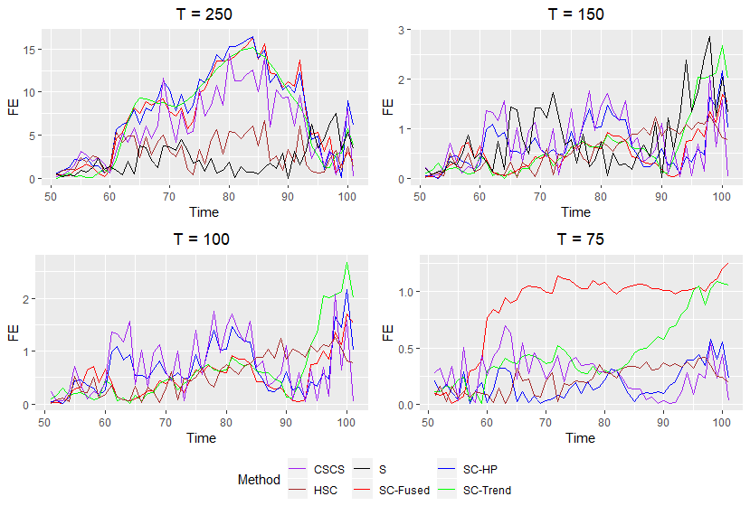
We compare the forecast performance of six covariance estimators (SC (HP, Fused, Trend), CSCS, HSC, and S) by using training and test datasets described above. The sample mean and covariance matrix are computed from the training data for each . Using (19), the 51 first half of a day arrival counts were used to forecast the second half of the day arrival counts. For each time interval , we define the forecast error (FE) by the average
where and are the observed and forecast values, respectively (Huang et al. 2006).
| Training data size | ||||
| Method | 205 | 150 | 100 | 75 |
| SC-HP | 1 | 5 | 9 | 20 |
| SC-Fused | 3 | 7 | 2 | 3 |
| SC-Trend | 7 | 8 | 16 | 1 |
| CSCS | 3 | 8 | 10 | 15 |
| HSC | 12 | 13 | 14 | 12 |
| S | 25 | 10 | - | - |
Table 3 reports the number of times each of the six forecast methods has the minimum forecast error values out of the total 51 trials. The maximum of the number of times the method achieves the minimum forecast error in each column is in bold. When and the training data size is larger than the number of variables, the forecast based on the Sample covariance matrix performs the best in terms of the number of times it achieves the minimum forecast error. For , the HSC is a bit better than the sample covariance matrix. However, as the training data size decreases, the forecasting ability of the SC algorithm increases. In particular, the SC-Trend and HP report the best result in terms of the number of times they achieve the minimum forecast error for and , respectively. Most of the result in Table 3 is supported by the aggregate forecast errors reported in Table 4, where aggregate forecast error is the sum of forecasted errors over . The minimum aggregate forecast error the method achieves is in bold. The discrepancies between Table 3 and Table 4 can be explained by looking on Figure 11, which illustrates a plot of for varying values of the training data size. For example, for the HSC achieves the minimum forecast error the most in terms of the number of times, however SC-Fused is the lowest in terms of the aggregate forecast error. This discrepancy explained from the top right plot of Figure 11, where it can be seen that when the of HSC is lowest, the of SC-Fused does not concede to much, but when the of SC-Fused is the lowest, HSC takes higher values, which forces the aggregate error of SC-Fused to be lower than the error of HSC,
| Training data size | ||||
|---|---|---|---|---|
| Methods | 205 | 150 | 100 | 75 |
| SC-HP | ||||
| SC-Fused | ||||
| SC-Trend | ||||
| CSCS | ||||
| HSC | ||||
| S | ||||
An R (R Core Team 2019) package, named SC, is available on Github repository (Dallakyan 2019). The core functions are coded in C++, allowing us to solve large-scale problems in substantially less time.
5 Conclusion
This paper proposes a novel penalized likelihood approach for smooth Cholesky-based covariance (inverse) estimation for longitudinal data or when a natural ordering among the variables is available. We reparameterize the normal likelihood in terms of the standard Cholesky factor (Khare et al. 2019) and rely on fused-type Lasso penalties to formulate jointly convex objective functions. A block coordinate descent algorithm is proposed to minimize the objective function. We establish convergence of the algorithm which always leads to positive-definite estimate of the covariance matrix. A goal of the study was to explore the connection between the local stationarity of a time series and smoothness of the subdiagonals of the Cholesky factor of its (inverse) covariance matrix. A connection between subdiagonal smoothness of the standard Cholesky factor and the modified factor is established. The performance of our methodology is illustrated via various simulations and two datasets.
6 Supporting Information
Additional Supporting Information may be found online in the supporting information tab for this article.
7 Data Availability Statement
Cattle data that supports the findings of this study are available as supporting information online, while Call Center data are available on request from the corresponding author. The latter data are not publicly available due to privacy or ethical restrictions.
Appendix A Proof of Lemma 1
(a):
We use the selection matrices which are submatrices of the identity matrix with row indices in such that . Then it is evident that and a compatible partition of leads to
| (20) | ||||
Note that the submatrix is diagonal with positive entries, and the matrix has nonzero values in the entries, which correspond to the diagonal of the submatrix of .
(b):
(c):
Since is positive definite, then as the sum of strictly convex and convex functions, is strictly convex (Boyd and Vandenberghe 2004).
Appendix B Proof of Lemma 2
(a):
The derivative with respect to of the quadratic form in (9) is
| (22) |
where is the vector with th element equal to 1 and 0 otherwise. By construction, the matrix is diagonal and the first element of is 0, so that the first identity in (22) is
Similarly, for the rows, we have
where its non-negative solution is as given in (12).
(b):
In (10), is a diagonal matrix with positive entries, setting and completing the square, then finding is equivalent to solving a generalized lasso problem:
| (23) |
which has a unique solution Tibshirani and Taylor 2011.
(c):
(1):
Proof is similar to the transformation in part (b).
(2):
Setting the derivative of to zero and solving for gives
The matrix inverse can be computed in flops Golub and Van Loan 1996, since is diagonal and is a tridiagonal matrix. Here is the length of the vector .
(d):
Proof of the lemma is similar to Friedman et al. 2007, thus omitted.
Appendix C Proof of Theorem 1
(a):
Recall that where is the vector of th subdiagonal. To make a change of variables in terms of difference of successive subdiagonal terms, define , where . Then, we have where is a block diagonal matrix where the th block is a lower triangular matrix with ones as the nonzero entries. Substituting for in , we get
| (24) |
where is the submatrix that selects the rows and columns of with indices in . Next, we rewrite
| (25) |
where , ,
and the set corresponds to the indices of the difference terms in .
The matrix is positive semi-definite, since it is a submatrix of the positive semi-definite matrix obtained by selecting specific rows and columns . Therefore, from Horn and Johnson 2012 the matrix is positive semi-definite and can be written as (Horn and Johnson 2012, Chapter 7) which establishes the equivalency of and (15). Since the diagonal elements of the sample covariance matrix is assumed to be positive, then and hence do not have 0 columns.
We note that (25) is not a fully form of (14), since the penalty reformulation involves of the components in each subdiagonal . However, with the transformation similar to Rojas and Wahlberg 2014 easily formulate (25) as (14).
(b):
We show the convergence of iterates produced by Algorithm 1 to a global minimum by invoking Khare and Rajaratnam 2014.
From Part (a) of the Theorem, there exist matrix with no 0 columns such that (15 holds and Lemma 3 shows an existence of an uniform lower bound for . Thus, to show convergence, it suffices to show that the assumption (A5)* Khare and Rajaratnam 2014 is satisfied or the level set of , is bounded. The latter property follows from the coercive property of the established in Lemma 3, since the level sets of coercive function are bounded (Bertsekas 2016).
Appendix D Proof of Lemma 3
In objective function , and the eigenvalues of a lower triangular matrix are its diagonal elements, then from the well-known inequality it follows that
Thus
where the equality in (*) follows from completing the square by adding and subtracting and writing . The inequality in (**) follows by completing the middle term as square and noting that is positive semi-definite (the Schur complement of the positive semi-definite matrix ) and (***) is based on the triangle inequality .
It follows from (**) and (***) that as any subdiagonal , and that if any diagonal element then . Therefore, any global minimum of has a strictly positive values for and hence any global minimum of over the open set lies in . Here, is open in the set of all lower triangular matrices. Moreover, from the discussion above the function is coercive, i.e. if , then .
Appendix E Convergence of -trend filtering and HP
The convergence proof of trend filtering follows the same steps as described in previous section. For this case, the change of variables occurs by taking as a block diagonal matrix where the th block is a lower triangular matrix with the sequence as a nonzero elements in th column (Kim et al. 2009, Section 3.2). The rest of the proof is similar to Appendix C, thus omitted.
For the convergence of HP, we note that for this case is convex differentiable function and the existing literature can be used to show convergence. For example see Luo and Tseng 1992.
Appendix F Proof of Lemma 4
We use ideas similar to the Friedman et al. 2010; Cai et al. 2011; Khare et al. 2019. We start by considering two cases
Case 1 ()
Each iteration of SC Algorithm sweeps over diagonal and subdiagonal elements. Thus, update of the diagonal consists of estimating and then computing diagonal using Lemma 2. From the discussion provided before the Theorem 1, recall that matrix is diagonal and has nonzero elements located in separate columns, for . Thus the complexity of computing in SC algorithm is
From the Lemma 2, the computational cost of estimating diagonal is . Therefore the cost of diagonal update can be done in steps.
The update of each subdiagonal consist of computing and estimating the subdiagonal in SC algorithm. Thus, the cost of estimating is
and since each iteration sweeps over subdiagonals we have
Case 2 ()
We use similar technique as in Khare et al. 2019. Note that, since , where matrix, then , where . Moreover , where is submatrix whose rows were selected from index . Recall and let , which takes iterations, due to sparsity structure of . Given initial value , we evaluate and keep truck of . If and differ only in one block coordinate , then
| (26) |
for . Therefore it takes computations to update to . Hence, after each block update in SC algorithm, it will take computations to update to its current value. Thus, the computation of can be transformed into
| (27) |
for . It follows the update of k’th block in (26), consequently in (27) takes computations. Hence one iteration will take computations.
Appendix G Proof of Lemma 5
(a):
(b):
The bounded total variation of follows from the fact that it is product of two functions of bounded total variation (Grady 2009, Theorem 2.4) and (16) follows from summing (28) over
Appendix H Proof of Proposition 1
We say that the matrix belongs to the class if its diagonal and subdiagonals are functions of bounded variation. The following notation introduced in Golub and Van Loan 1996 simplifies the discussion of the proof. For we introduce the matrix , which has the same th sub(sup)diagonal as and 0 elsewhere. Clearly, if then . For the lower triangular matrix we have
and
From the structure of ’s it can be seen that the th subdiagonal of can be written as the sum of the th subdiagonals of the following matrix products
| (29) |
where from the position of degenerate values, the matrix product has nonzero values on the th subdiagonal and zero elsewhere. Moreover, nonzero values in the th subdiagonal of . Now, since the product of two functions of total bounded variation are of bounded variation and after adding and subtracting corresponding terms as in the proof of Lemma 5, we get
and the result follows from (29).
(b)
We show the converse of the part (a), i.e. if then there exist a unique and . The proof uses similar argument proposed in (Chern and Dieci 2000, Lemma 2.8). Before introducing the main argument, we state the following lemma, which will be used in the proof.
Lemma 6.
If lower triangular matrices then
Proof.
Using the matrix notation introduced in part(a), it can be shown that the th subdiagonal of the matrix product can be written as
and the result follows by recalling that the product of the functions of bounded variation is of bounded variation. ∎
The main argument consist in writing and let . From the construction of and , it is easy to see that and , where . Clearly, since by construction and . By repeating this procedure and using Lemma 6, result follows.
Appendix I Selection of Tuning Parameter
We use BIC-like measure and cross-validation to choose the tuning parameter . In particular, the tuning parameter is determined by choosing the minimum of BIC-like measure and CV over the grid. BIC is defined as:
where denoted the degrees of freedom, and are the sample size and covariance matrix, respectively. For example for the sparse fused lasso, corresponds to number of nonzero fused groups in (Tibshirani and Taylor 2011).
For fold cross-validation, we randomly split the full dataset into subsets of about the same size, denoted by . For each , is used to estimate the parameters and to validate. The performance of the model is measured using the log-likelihood. We choose the tuning parameter as a minimum of the fold cross-validated log-likelihood criterion over the grid.
where is the estimated Cholesky factor using the data set , is the index set of the data in , is the size of , and is the th observation of the dataset .
Appendix J Additional Simulation
In this section we provide additional simulation results. Two different cases are considered. In the first case, matrix is full lower triangular matrix and subdiagonals are randomly chosen from the Cases (A-D) described in the Section 4. In the second case, matrix follows nonhierarchical structure, in a sense described in Yu and Bien 2017. That is, in a full lower triangular matrix , we enforce first and last subdiagonals admit nonzero values, drawn from uniform [0.1, 0.2] and positive/negative signs are then assigned with probability 0.5. The rest of subdiagonals admit zero value. See Figure 14 for an illustration. For the latter case, Sparse SC have been used for the estimation. That is we use two tuning parameters to control sparsity and smoothness, respectively.
For both cases, we consider settings when and , however because of the space limitation only is reported. Each possible setting is repeated over 20 simulated datasets. The tuning parameters were chosen using cross-validation. Moreover, for the second case we compare the results from sparse SC (HP, Fused, Trend) estimator with CSCS and HSC using a receiver operating characteristic curve, or ROC curve.
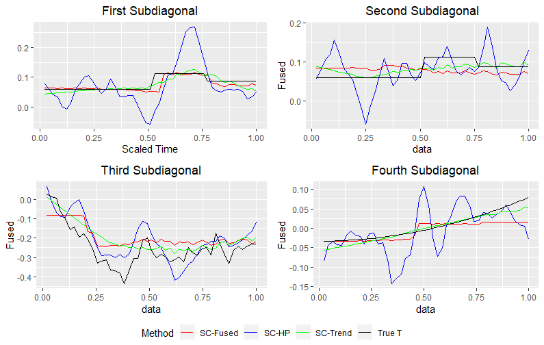
We start by providing results for the first case. The Figure 12 plots the first four estimated subdiagonals of the full lower traingular matrix , using SC estimator. From the figure, the first two subdiagonals correspond to the Case B, the third to the Case D and the fourth to the Case C, respectively. Visually, the SC-Fused captures the step function the best for the first subdiagonal. However, all three estimators failed to capture the stepwise linear structure of the second subdiagonal, but there is a significant improvement of SC estimator to capture the wiggliness of the Markov process in the third subdiagonal (SC-HP being the best) and smooth, slow time-varying structure of the fourth subdiagonal (SC-Trend being the best). Next we report the performance of three estimators using Frobenius and Infinity norm. Figure 13 plots the results. Overall, for matrix , SC-Trend filtering provides the lowest Frobenius and Infinity norm followed by SC-Fused.

Remark 1.
Relying on the result above, one can learn the lower triangular matrix () by considering the penalty form as an additional parameter to tune for each subdiagonal.
Now, we compare the performance of the SC with the CSCS and HSC on the support recovery, when the structure is non-hierarchical. Comparison is implemented using ROC curves. The ROC curve is created by plotting the true positive rate (TPR) against the false positive rate (FPR) at various penalty parameter settings (Friedman et al. 2010). Here, the ROC curve is obtained by varying around 60 possible values for the penalty parameter . For the SC-Fused, Trend and HP, the smoothing tuning parameter is obtained from the cross-validation by fixing in a given value. In applications, FPR is usually controlled to be sufficiently small, thus following Khare et al. 2019, the focus is on comparing portion of ROC curves for which FPR is less than 0.15. The comparison of ROC curves is implemented using Area-under-the-curve (AUC) (Friedman et al. 2010).
Table 5 reports the mean and the standard deviation (over 20 simulations) for the AUCs for SC (HP, Fused and Trend), CSCS and HSC when and . The best result is given in bold.
| Method | Mean | Std. Dev |
|---|---|---|
| SC-HP | ||
| SC- Fused | ||
| SC- Trend | ||
| CSCS | ||
| HSC |
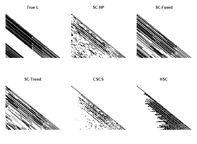
From the table above, it can be seen that HSC provides the best result. However, Figure 14, which captures snapshot of the graphical comparison of the estimated matrix for the five estimators, sheds more lights into characteristics of estimators. As can be seen, even though HSC provides the highest AUC for FPR less than 0.15, it fails to capture the zero gap between subdiagonals of matrix compare, for example, with SC-Fused, which provides the second best result in the Table 5.
Appendix K Cattle data: Additional Analysis
Figure 15 provides the plot of the first two subdiagonals using eight estimators descirbed in Section 4.5.

References
- Adak (1998) Adak, Sudeshna (1998), “Time-dependent spectral analysis of nonstationary time series.” Journal of the American Statistical Association, 93, 1488–1501.
- Ansley (1979) Ansley, Craig F. (1979), “An algorithm for the exact likelihood of a mixed autoregressive-moving average process.” Biometrika, 66, 59–65.
- Banerjee et al. (2008) Banerjee, Onureena, Laurent El Ghaoui, and Alexandre d’Aspremont (2008), “Model selection through sparse maximum likelihood estimation for multivariate gaussian or binary data.” J. Mach. Learn. Res., 9, 485–516.
- Bertsekas (2016) Bertsekas, D.P. (2016), Nonlinear Programming. Athena Scientific.
- Bickel and Gel (2011) Bickel, Peter J. and Yulia R. Gel (2011), “Banded regularization of autocovariance matrices in application to parameter estimation and forecasting of time series.” Journal of the Royal Statistical Society: Series B (Statistical Methodology), 73, 711–728.
- Blake (2018) Blake, Tayler (2018), Nonparametric Covariance Estimation with Shrinkage toward Stationary Models. Ph.D. thesis, The Ohio State University.
- Boyd and Vandenberghe (2004) Boyd, Stephen and Lieven Vandenberghe (2004), Convex Optimization. Cambridge University Press, New York, NY, USA.
- Cai et al. (2011) Cai, Tony, Weidong Liu, and Xi Luo (2011), “A constrained l1 minimization approach to sparse precision matrix estimation.” Journal of the American Statistical Association, 106, 594–607. Available at https://doi.org/10.1198/jasa.2011.tm10155.
- Chern and Dieci (2000) Chern, Jann-Long and Luca Dieci (2000), “Smoothness and periodicity of some matrix decompositions.” SIAM J. Matrix Analysis Applications, 22, 772–792.
- Dahlhaus (1997) Dahlhaus, R. (1997), “Fitting time series models to nonstationary processes.” Ann. Statist., 25, 1–37. Available at https://doi.org/10.1214/aos/1034276620.
- Dahlhaus (2012) Dahlhaus, Rainer (2012), “Locally stationary processes.” Handbook of Statistics, 30, 351–413.
- Dahlhaus and Polonik (2009) Dahlhaus, Rainer and Wolfgang Polonik (2009), “Empirical spectral processes for locally stationary time series.” Bernoulli, 15, 1–39.
- Dai and Guo (2004) Dai, Ming and Wensheng Guo (2004), “Multivariate spectral analysis using cholesky decomposition.” Biometrika, 91, 629–643.
- Dallakyan (2019) Dallakyan, Aramayis (2019), “Sc package.” https://github.com/adallak/SCPackage.
- Das and Politis (2020) Das, Srinjoy and Dimitris N. Politis (2020), “Predictive inference for locally stationary time series with an application to climate data.” Journal of the American Statistical Association, 0, 1–16.
- Davis et al. (2006) Davis, A Richard, C. M Thomas Lee, and Rodriguez-Yam A Gabriel (2006), “Structural break estimation for nonstationary time series models.” Journal of the American Statistical Association, 101, 223–239.
- Friedman et al. (2010) Friedman, H. Jerome, J. Trevor Hastie, and Robert Tibshirani (2010), “Applications of the lasso and grouped lasso to the estimation of sparse graphical models.” Available at http://statweb.stanford.edu/~tibs/ftp/ggraph.pdf.
- Friedman et al. (2008) Friedman, J, T Hastie, and R. Tibshirani (2008), “Sparse inverse covariance estimation with the graphical lasso.” Biostatistics, 9, 432–441.
- Friedman et al. (2007) Friedman, Jerome, Trevor Hastie, Holger Höfling, and Robert Tibshirani (2007), “Pathwise coordinate optimization.” Ann. Appl. Stat., 1, 302–332.
- Gabriel (1962) Gabriel, K. R. (1962), “Ante-dependence analysis of an ordered set of variables.” Ann. Math. Statist., 33, 201–212.
- Golub and Van Loan (1996) Golub, Gene H. and Charles F. Van Loan (1996), Matrix Computations (3rd Ed.). Johns Hopkins University Press, Baltimore, MD, USA.
- Grady (2009) Grady, Noella (2009), “Functions of bounded variation.” Available at https://www.whitman.edu/Documents/Academics/Mathematics/grady.pdf.
- Hodrick and Prescott (1997) Hodrick, Robert J. and Edward Prescott (1997), “Postwar u.s business cycles: An empirical investigation.” Journal of Money, Credit and Banking, 29.
- Horn and Johnson (2012) Horn, Roger A. and Charles R. Johnson (2012), Matrix Analysis, 2nd edition. Cambridge University Press, New York, NY, USA.
- Huang et al. (2006) Huang, J, N Liu, M Pourahmadi, and L. Liu (2006), “Covariance matrix selection and estimation via penalised normal likelihood.” Biometrika, 93, 85–98.
- Huang et al. (2007) Huang, Z Jianhua, Linxu Liu, and Naiping Liu (2007), “Estimation of large covariance matrices of longitudinal data with basis function approximations.” Journal of Computational and Graphical Statistics, 16, 189–209.
- Kenward (1987) Kenward, Michael G. (1987), “A method for comparing profiles of repeated measurements.” Journal of the Royal Statistical Society. Series C (Applied Statistics), 36, 296–308.
- Khare et al. (2019) Khare, Kshitij, Sang-Yun Oh, Syed Rahman, and Bala Rajaratnam (2019), “A scalable sparse cholesky based approach for learning high-dimensional covariance matrices in ordered data.” Machine Learning, 108, 2061–2086.
- Khare et al. (2015) Khare, Kshitij, Sang-Yun Oh, and Bala Rajaratnam (2015), “A convex pseudolikelihood framework for high dimensional partial correlation estimation with convergence guarantees.” Journal of the Royal Statistical Society: Series B (Statistical Methodology), 77, 803–825.
- Khare and Rajaratnam (2014) Khare, Kshitij and Bala Rajaratnam (2014), “Convergence of cyclic coordinatewise l1 minimization.” arXiv e-prints. Available at https://arxiv.org/pdf/1404.5100.pdf.
- Kim et al. (2009) Kim, Seung-Jean, Kwangmoo Koh, Stephen P Boyd, and Dimitry M. Gorinevsky (2009), “l1 trend filtering.” SIAM Review, 51, 339–360.
- Kitagawa and Gersch (1985) Kitagawa, G. and W. Gersch (1985), “A smoothness priors time-varying ar coefficient modeling of nonstationary covariance time series.” IEEE Transactions on Automatic Control, 30, 48–56.
- Levina et al. (2008) Levina, Elizaveta, Adam Rothman, and Ji Zhu (2008), “Sparse estimation of large covariance matrices via a nested lasso penalty.” 2, 245–263.
- Luo and Tseng (1992) Luo, Z. Q. and P. Tseng (1992), “On the convergence of the coordinate descent method for convex differentiable minimization.” Journal of Optimization Theory and Applications, 72, 7–35.
- McMurry and Politis (2010) McMurry, Timothy L. and Dimitris N. Politis (2010), “Banded and tapered estimates for autocovariance matrices and the linear process bootstrap.” Journal of Time Series Analysis, 31, 471–482.
- McMurry and Politis (2015) McMurry, Timothy L. and Dimitris N. Politis (2015), “High-dimensional autocovariance matrices and optimal linear prediction.” Electron. J. Statist., 9, 753–788.
- Peng et al. (2009) Peng, Jie, Pei Wang, Nengfeng Zhou, and Ji Zhu (2009), “Partial correlation estimation by joint sparse regression models.” Journal of the American Statistical Association, 104, 735–746.
- Pourahmadi (2001) Pourahmadi, M. (2001), Foundations of time series analysis and prediction theory. John Wiley & Sons, Ltd.
- Pourahmadi (1999) Pourahmadi, Mohsen (1999), “Joint mean-covariance models with applications to longitudinal data: Unconstrained parameterisation.” Biometrika, 86, 677–690.
- Pourahmadi (2013) Pourahmadi, Mohsen (2013), High-Dimensional Covariance Estimation. John Wiley & Sons, Ltd.
- R Core Team (2019) R Core Team (2019), R: A Language and Environment for Statistical Computing. R Foundation for Statistical Computing, Vienna, Austria, URL http://www.R-project.org/.
- Rao (1970) Rao, T. Subba (1970), “The fitting of non-stationary time-series models with time-dependent parameters.” Journal of the Royal Statistical Society. Series B (Methodological), 32, 312–322.
- Rojas and Wahlberg (2014) Rojas, Cristian R. and Bo Wahlberg (2014), “On change point detection using the fused lasso method.”
- Rosen and Stoffer (2007) Rosen, Ori and David S. Stoffer (2007), “Automatic estimation of multivariate spectra via smoothing splines.” Biometrika, 94, 335–345.
- Rothman et al. (2010) Rothman, J. Adam, Elizaveta Levina, and Ji Zhu (2010), “A new approach to cholesky-based covariance regularization in high dimensions.” Biometrika, 97, 539–550.
- Rudin et al. (1992) Rudin, Leonid I., Stanley Osher, and Emad Fatemi (1992), “Nonlinear total variation based noise removal algorithms.” Physica D: Nonlinear Phenomena, 60, 259 – 268.
- Shojaie and Michailidis (2010) Shojaie, Ali and George Michailidis (2010), “Penalized likelihood methods for estimation of sparse high-dimensional directed acyclic graphs.” Biometrika, 97, 519–538.
- Tibshirani et al. (2005) Tibshirani, Robert, Michael Saunders, Saharon Rosset, Ji Zhu, and Keith Knight (2005), “Sparsity and smoothness via the fused lasso.” Journal of the Royal Statistical Society, 67, 91–108.
- Tibshirani and Taylor (2011) Tibshirani, Ryan J. and Jonathan Taylor (2011), “The solution path of the generalized lasso.” Ann. Statist., 39, 1335–1371.
- Whittaker (1990) Whittaker, J. (1990), Graphical models in applied multivariate statistics. John Wiley & Sons, Ltd.
- Wu and Pourahmadi (2003) Wu, Wei Biao and Mohsen Pourahmadi (2003), “Nonparametric estimation of large covariance matrices of longitudinal data.” Biometrika, 90, 831–844.
- Wu and Pourahmadi (2009) Wu, Wei Biao and Mohsen Pourahmadi (2009), “Banding sample autocovariance matrices of stationary processes.” Statistica Sinica, 19, 1755–1768.
- Yu and Bien (2017) Yu, Guo and Jacob Bien (2017), “Learning local dependence in ordered data.” Journal of Machine Learning Research, 18, 1–60.
- Zimmerman and Nunez-Anton (2010) Zimmerman, Dale L. and Vicente A. Nunez-Anton (2010). Chapman & Hall/CRC Monographs on Statistics & Applied Probability, Taylor & Francis, New York.