Output Based Adaptive Distributed Output Observer for Leader-follower Multiagent Systems^footnoteinfo

He Cai Email: caihe@scut.edu.cn Jie Huang Email: jhuang@mae.cuhk.edu.hk

Abstract

The adaptive distributed observer approach has been an effective tool for synthesizing a distributed control law for solving various control problems of leader-follower multiagent systems. However, the existing adaptive distributed observer needs to make use of the full state of the leader system. This assumption not only precludes many practical applications in which only the output of the leader system is available, but also leads to a high dimension observer. In this communique, we propose an adaptive distributed output observer which only makes use of the output of the leader system, and is thus more practical than the state based adaptive distributed observer. Moreover, the dimension and the information exchange among agents of the proposed adaptive distributed output observer can be significantly smaller than those of the state based adaptive distributed output observer.

keywords

Adaptive distributed output observer, output feedback control, multiagent system.

^†^†thanks: [^†^†address: Department of Mechanical and Automation Engineering, The Chinese University of Hong Kong, Shatin, N.T., Hong Kong.

footnoteinfo]This work has been supported in part by the Research Grants Council of the Hong Kong Special Administration Region under grant No. 14201418, and in part by National Natural Science Foundation of China under grant No. 61973260. Corresponding author: J. Huang. Tel. +852-39438473. Fax +852-39436002.

, .

1 Introduction

The past decade has witnessed a significant advancement on the research of multiagent systems [3, 8, 9, 11, 13, 14, 15]. A variety of approaches have been developed for handling various control problems. One of the systematic and effective approaches for the control of leader-follower multiagent systems is the so-called distributed observer approach [18], which consists of two design steps. First, a distributed observer is synthesized for the given leader system. This distributed observer will provide the estimation of the leader’s state to each follower system satisfying the communication constraints. Second, based on the estimated leader’s state provided by the distributed observer, a certainty equivalent control law is synthesized for each follower to achieve the control objective. A typical example of the application of the distributed observer approach can be found in [4], where the distributed observer was used to recover the reference signals for solving the distributed robust tracking problem of a leader-follower Euler-Lagrange multiagent system.

Nevertheless, the distributed observer approach has one drawback in that it assumes that the control law of each follower knows the leader’s system matrix, which may not be desirable in some practical applications. To remove this assumption, the adaptive distributed observer approach was further proposed in [2], which not only estimates the state of the leader system but also the system matrix of the leader system. As a result, the assumption that all the followers know the leader’s system matrix is removed, which enables the design of a fully distributed control law. Some other variants on the adaptive distributed observer approach, such as the one that guarantees finite time convergence and the one that deals with multiple leaders, can be found in [7, 12].

Both the existing distributed observers and adaptive distributed observers need to make use of the full state of the leader system. This assumption not only precludes many practical applications in which only the output of the leader system is available, but also leads to a high dimension observer. In this communique, we propose an output based adaptive distributed output observer depending solely on the output of the leader system, which is the only practical solution in case where the state of the leader is not available. Moreover, instead of estimating every entry of the leader’s system and output matrices, we only estimate the coefficients of the minimal polynomial of the leader’s system matrix. As a result, both the dimension and the information exchange among agents of the proposed output based adaptive distributed output observer can be drastically smaller than those of the state based adaptive distributed output observer.

The rest of this communique is organized as follows. Notation and preliminaries are summarized in Section 2. Section 3 presents the design of the output based adaptive distributed output observer. A numerical example is given in Section 4. Section 5 concludes this communique.

2 Notation and Mathematical Preliminaries

2.1 Notation

$\mathbb{R}$ and $\mathbb{C}$ denote the sets of real and complex numbers, respectively. For $x\in\mathbb{C}$ , $\Re(x)$ denotes the real part of $x$ . $1_{N}$ denotes an $N$ dimensional column vector whose components are all $1$ . $||x||$ denotes the Euclidean norm of a vector $x$ . $||A||$ denotes the Euclidean norm of a matrix $A$ . $A^{T}$ ( $A^{H}$ ) denotes the (Hermitian) transpose of $A$ . For a square matrix $A$ , $\sigma(A)$ denotes the spectrum of $A$ , $\Re(\sigma(A))$ denotes the set of the real parts of all the elements of $\sigma(A)$ , $\bar{\delta}_{A}=\max(\Re(\sigma(A)))$ , $\underline{\delta}_{A}=\min(\Re(\sigma(A)))$ , and $A>0$ $(A\geq 0)$ means $A$ is positive definite (positive semi-definite). A matrix $A=[a_{ij}]\in\mathbb{R}^{n\times n}$ is called an $M$ -matrix if $a_{ij}\leq 0$ for $i\neq j$ and $\underline{\delta}_{A}>0$ . For two hermitian matrices $X_{1}$ and $X_{2}$ , $X_{1}\leq X_{2}$ means $X_{2}-X_{1}\geq 0$ . Given a time-varying matrix $A(t)$ , if $||A(t)||\leq\beta e^{-\alpha t}$ for some $\alpha,\beta>0$ , then $A(t)$ is said to decay to zero exponentially at the rate of $\alpha$ . $\otimes$ denotes the Kronecker product of matrices. For $x_{i}\in\mathbb{R}^{n_{i}}$ , $i=1,\dots,m$ , $\hbox{col}(x_{1},\dots,x_{m})=[x_{1}^{T},\dots,x_{m}^{T}]^{T}$ .

2.2 Preliminaries

First, we list two lemmas for convenience of the readers.

Lemma 2.1

Given a detectable pair $(C,A)$ , where $A\in\mathbb{R}^{n\times n}$ , $C\in\mathbb{R}^{m\times n}$ , let $P>0$ be the unique solution of the algebraic Riccati equation

PA^{T}+AP-PC^{T}CP+Q=0

(1)

for some $Q>0$ . Let $\Phi=I_{N}\otimes A-\mu(F\otimes PC^{T}C)$ where $F\in\mathbb{R}^{N\times N}$ satisfies $\underline{\delta}_{F}>0$ . Then, $\Phi$ is Hurwitz if $\mu>\underline{\delta}_{F}^{-1}$ .

The proof of Lemma 2.1 can be extracted from the proof of Theorem 2 of [19].

Lemma 2.2

(p.168, p.260, Theorem 11.2.1 of [10]) Consider the following equation

XDX-XA-A^{H}X-C=0

(2)

where $A,C,D,X\in\mathbb{C}^{n\times n}$ . A hermitian solution $X_{+}$ of (2) is called maximal if $X\leq X_{+}$ for every hermitian solution $X$ of (2). $X_{+}$ as a function of $A$ , $C$ and $D$ is expressed as $X_{+}=X_{+}(A,C,D)$ . Let $\mathds{P}$ denote the set of all ordered triples $(A,C,D)$ satisfying $D\geq 0$ , $C=C^{H}$ , $(A,D)$ is stabilizable, and (2) admits hermitian solutions. Then, the maximal hermitian solution $X_{+}(A,C,D)$ of (2) is a continuous function of $(A,C,D)\in\mathds{P}$ .

Next, we summarize the result from [2] regarding the adaptive distributed observer. Consider the linear system described as follows:


$\displaystyle\dot{v}_{0}$	$\displaystyle=S_{0}v_{0}$	(3a)
$\displaystyle y_{0}$	$\displaystyle=C_{0}v_{0}$	(3b)

where $v_{0}\in\mathbb{R}^{q}$ , $y_{0}\in\mathbb{R}^{p}$ , $S_{0}\in\mathbb{R}^{q\times q}$ and $C_{0}\in\mathbb{R}^{p\times q}$ are constant matrices.

Let $\bar{\mathcal{G}}=(\bar{\mathcal{V}},\bar{\mathcal{E}})$ denote a digraph¹¹ 1 See Notation of [2] for a summary of graph notation. with $\bar{\mathcal{V}}=\{0,1,\dots,N\}$ . Here the node $0$ is associated with the leader system (3) and node $i$ is associated with the $i$ th follower. It is assumed that the digraph $\bar{\mathcal{G}}=(\bar{\mathcal{V}},\bar{\mathcal{E}})$ satisfies the following assumption:

Assumption 1

The communication graph $\bar{\mathcal{G}}$ contains a spanning tree with the node $0$ as the root.

Remark 2.1

Assumption 1 is a standard and necessary assumption for the control of the leader-follower multiagent systems under static network topology. Let $\bar{\mathcal{L}}$ be the Lapacian of $\bar{\mathcal{G}}$ , and $H$ consist of the last $N$ rows and the last $N$ columns of $\bar{\mathcal{L}}$ . Then, by Lemma 4 of [6] or Lemma 1 of [18], under Assumption 1, $-H$ is Hurwitz. Thus, $\underline{\delta}_{H}>0$ .

Given the system (3) and the graph $\bar{\mathcal{G}}$ , we established the adaptive distributed observer for the leader system in [1] as follows:


$\displaystyle\dot{S}_{i}$	$\displaystyle=\mu_{s}\sum_{j=0}^{N}a_{ij}(S_{j}-S_{i})$	(4a)
$\displaystyle\dot{C}_{i}$	$\displaystyle=\mu_{c}\sum_{j=0}^{N}a_{ij}(C_{j}-C_{i})$	(4b)
$\displaystyle\dot{v}_{i}$	$\displaystyle=S_{i}v_{i}+\mu_{v}\sum_{j=0}^{N}a_{ij}(v_{j}-v_{i})$	(4c)

where $S_{i}\in\mathbb{R}^{q\times q}$ , $C_{i}\in\mathbb{R}^{p\times q}$ , $v_{i}\in\mathbb{R}^{q}$ , $\mu_{s},\mu_{c},\mu_{v}>0$ . Let $y_{i}=C_{i}v_{i}$ , $\tilde{y}_{i}=y_{i}-y_{0}$ , $\tilde{S}_{i}=S_{i}-S_{0}$ , $\tilde{v}_{i}=v_{i}-v_{0}$ , $\tilde{C}_{i}=C_{i}-C_{0}$ , $i=1,\dots,N$ . Noting that $\tilde{y}_{i}=C_{i}\tilde{v}_{i}+\tilde{C}_{i}v_{0}$ , by Lemma 2 of [2], we can obtain the following result:

Lemma 2.3

Given system (4), under Assumption 1, for all $v_{i}(0)\in\mathbb{R}^{q}$ , $i=0,1,\dots,N$ , $S_{i}(0)\in\mathbb{R}^{q\times q}$ , $C_{i}(0)\in\mathbb{R}^{p\times q}$ , $i=1,\dots,N$ , we have

(i): for any $\mu_{s},\mu_{c}>0$ , $S_{i}(t)$ and $C_{i}(t)$ exist for all $t\geq 0$ and satisfy $\lim_{t\rightarrow\infty}\tilde{S}_{i}(t)=0$ , $\lim_{t\rightarrow\infty}\tilde{C}_{i}(t)=0$ exponentially at the rate of $\mu_{s}\underline{\delta}_{H}$ , $\mu_{c}\underline{\delta}_{H}$ , respectively;
(ii): if $\mu_{s},\mu_{c},\mu_{v}>\bar{\delta}_{S_{0}}\underline{\delta}_{H}^{-1}$ , then $y_{i}(t)$ exists for all $t\geq 0$ and satisfies $\lim_{t\rightarrow\infty}\tilde{y}_{i}(t)=0$ exponentially.

Remark 2.2

The adaptive distributed output observer (4) was first proposed in [2] for the special case where the matrix $C_{0}$ in (3) is an identity matrix. For this special case, $y_{0}=v_{0}$ . Thus, there is no need to estimate $C_{0}$ in order to recover $y_{0}$ , and the adaptive distributed observer given in [2] consists of only (4a) and (4c). Since (4) assumes that the state $v_{0}$ of the leader system is available, it can be more precisely called state based adaptive distributed output observer.

3 Main Result

In this section, we offer two significant improvements over (4). First, (4) needs the full state of the leader system. But, in many practical applications, only the output of the leader system is available. Thus, we will propose a so-called output based adaptive distributed output observer that only relies on the output $y_{0}$ of the leader system. Second, all the entries of $S_{0}$ and $C_{0}$ need to be estimated by each follower using (4). In contrast, we will show that it suffices to estimate the coefficients of the minimal polynomial of $S_{0}$ instead of all the entries of $S_{0}$ and $C_{0}$ . Thus, the proposed output based adaptive distributed output observer can drastically reduce the dimension of the observer as well as the information exchange among agents.

Suppose the minimal polynomial of $S_{0}$ is given by $s^{n}+\alpha_{0,1}s^{n-1}+\cdots+\alpha_{0,n-1}s+\alpha_{0,n}$ . Then, by the Cayley-Hamilton Theorem,

S_{0}^{n}+\alpha_{0,1}S_{0}^{n-1}+\dots+\alpha_{0,n-1}S_{0}+\alpha_{0,n}I_{q}=0.

(5)

By (3), for $k=0,1,\dots,n$ ,

y_{0}^{(k)}=C_{0}S_{0}^{k}v_{0}.

(6)

Then

	$\displaystyle y_{0}^{(n)}+\alpha_{0,1}y_{0}^{(n-1)}+\dots+\alpha_{0,n-1}y_{0}^{(1)}+\alpha_{0,n}y_{0}$	(7)
$\displaystyle=$	$\displaystyle C_{0}S_{0}^{n}v_{0}+\alpha_{0,1}C_{0}S_{0}^{n-1}v_{0}+\cdots$
	$\displaystyle+\alpha_{0,n-1}C_{0}S_{0}v_{0}+\alpha_{0,n}C_{0}v_{0}$
$\displaystyle=$	$\displaystyle C_{0}(S_{0}^{n}+\alpha_{0,1}S_{0}^{n-1}+\dots+\alpha_{0,n-1}S_{0}+\alpha_{0,n}I_{q})v_{0}=0.$

Let $\zeta_{0}=\hbox{col}(y_{0},y_{0}^{(1)},\dots,y_{0}^{(n-1)})\in\mathbb{R}^{pn}$ . Then,

$\displaystyle\dot{\zeta}_{0}$	$\displaystyle=\left[\left(\begin{array}[]{cccc}0&&&\\ \vdots&&I_{n-1}&\\ 0&&&\\ -\alpha_{0,n}&\cdots&-\alpha_{0,2}&-\alpha_{0,1}\\ \end{array}\right)\otimes I_{p}\right]\zeta_{0}$	(8)
	$\displaystyle\triangleq\mathcal{S}_{0}\zeta_{0}$
$\displaystyle y_{0}$	$\displaystyle=\left[\left(\begin{array}[]{cccc}1&0&\cdots&0\\ \end{array}\right)\otimes I_{p}\right]\zeta_{0}\triangleq\mathcal{C}_{0}\zeta_{0}.$

Since $(\mathcal{C}_{0},\mathcal{S}_{0})$ is observable, let $\mathcal{P}_{0}>0$ be the unique solution of the algebraic Riccati equation

\mathcal{P}_{0}\mathcal{S}_{0}^{T}+\mathcal{S}_{0}\mathcal{P}_{0}-\mathcal{P}_{0}\mathcal{C}_{0}^{T}\mathcal{C}_{0}\mathcal{P}_{0}+I_{pn}=0.

(9)

Let $\alpha_{0}=\hbox{col}(\alpha_{0,1},\dots,\alpha_{0,n})$ . For $i=1,\dots,N$ , let

\dot{\alpha}_{i}=\mu_{\alpha}\sum_{j=0}^{N}a_{ij}(\alpha_{j}-\alpha_{i})

(10)

where $\alpha_{i}\in\mathbb{R}^{n}$ , $\mu_{\alpha}>0$ , and define

\mathcal{S}_{i}=\left(\begin{array}[]{cccc}0&&&\\ \vdots&&I_{n-1}&\\ 0&&&\\ -\alpha_{i,n}&\cdots&-\alpha_{i,2}&-\alpha_{i,1}\\ \end{array}\right)\otimes I_{p}.

(11)

Note that $(\mathcal{C}_{0},\mathcal{S}_{i}(t))$ is in the observable canonical form and thus is observable for all $t\geq 0$ . Therefore, the following algebraic Riccati equation

\mathcal{P}_{i}\mathcal{S}_{i}^{T}+\mathcal{S}_{i}\mathcal{P}_{i}-\mathcal{P}_{i}\mathcal{C}_{0}^{T}\mathcal{C}_{0}\mathcal{P}_{i}+I_{pn}=0

(12)

admits a unique solution $\mathcal{P}_{i}(t)>0$ for all $t\geq 0$ . For $i=1,\dots,N$ , let $\mathcal{F}_{i}=\mathcal{P}_{i}\mathcal{C}_{0}^{T}$ and define the following dynamic compensator

\dot{\zeta}_{i}=\mathcal{S}_{i}\zeta_{i}+\mu_{\zeta}\mathcal{F}_{i}\sum_{j=0}^{N}a_{ij}(y_{j}-y_{i})

(13)

where $\zeta_{i}\in\mathbb{R}^{pn}$ , $y_{i}=\mathcal{C}_{0}\zeta_{i}$ , $\mu_{\zeta}>0$ .

For $i=1,\dots,N$ , let $\tilde{\alpha}_{i}=\alpha_{i}-\alpha_{0}$ , $\tilde{\mathcal{S}}_{i}=\mathcal{S}_{i}-\mathcal{S}_{0}$ , $\tilde{\mathcal{P}}_{i}=\mathcal{P}_{i}-\mathcal{P}_{0}$ , $\tilde{\zeta}_{i}=\zeta_{i}-\zeta_{0}$ and $\tilde{y}_{i}=y_{i}-y_{0}$ . We have the following result.

Theorem 3.1

Given systems (3) and (10), (13), under Assumption 1, if $\mu_{\alpha}>\bar{\delta}_{S_{0}}\underline{\delta}_{H}^{-1}$ and $\mu_{\zeta}>\underline{\delta}_{H}^{-1}$ , then for any $v_{0}(0)\in\mathbb{R}^{q}$ , $\alpha_{i}(0)\in\mathbb{R}^{n}$ , $\zeta_{i}(0)\in\mathbb{R}^{pn}$ , $i=1,\dots,N$ , $\alpha_{i}(t)$ and $\zeta_{i}(t)$ exist for all $t\geq 0$ and satisfy $\lim_{t\rightarrow\infty}\tilde{\alpha}_{i}(t)=0$ , $\lim_{t\rightarrow 0}\tilde{\mathcal{S}}_{i}(t)=0$ , $\lim_{t\rightarrow 0}\tilde{\mathcal{P}}_{i}(t)=0$ , $\lim_{t\rightarrow\infty}\tilde{\zeta}_{i}(t)=0$ , $\lim_{t\rightarrow\infty}\tilde{y}_{i}(t)=0$ .

Proof: Let $\tilde{\alpha}=\hbox{col}(\tilde{\alpha}_{1},\dots,\tilde{\alpha}_{N})$ . Note that $\alpha_{i}$ is governed by (10), which is in the same form as (4a). Thus, by Part (i) of Lemma 2.3, under Assumption 1, for any $\mu_{\alpha}>0$ , $\tilde{\alpha}_{i}(t)$ decays to zero exponentially at the rate of $\mu_{\alpha}\underline{\delta}_{H}$ , which together with (11) implies $\tilde{\mathcal{S}}_{i}(t)$ decays to zero exponentially at the rate of $\mu_{\alpha}\underline{\delta}_{H}$ . Note that $\mathcal{P}_{i}(t)$ is unique for all $t\geq 0$ and thus is continuous in $\mathcal{S}_{i}$ by Lemma 2.2. Therefore, $\lim_{t\rightarrow\infty}\tilde{\mathcal{S}}_{i}(t)=0$ implies that $\lim_{t\rightarrow\infty}\tilde{\mathcal{P}}_{i}(t)=0$ . Moreover, by (8) and (13), we have

$\displaystyle\dot{\tilde{\zeta}}_{i}$	$\displaystyle=\mathcal{S}_{i}\zeta_{i}+\mu_{\zeta}\mathcal{F}_{i}\sum_{j=0}^{N}a_{ij}(y_{j}-y_{i})-\mathcal{S}_{0}\zeta_{0}$	(14)
	$\displaystyle=\mathcal{S}_{i}\zeta_{i}-\mathcal{S}_{0}\zeta_{i}+\mathcal{S}_{0}\zeta_{i}-\mathcal{S}_{0}\zeta_{0}$
	$\displaystyle+\mu_{\zeta}\mathcal{P}_{i}\mathcal{C}_{0}^{T}\mathcal{C}_{0}\sum_{j=0}^{N}a_{ij}(\zeta_{j}-\zeta_{i})$
	$\displaystyle=\mathcal{S}_{0}\tilde{\zeta}_{i}+\tilde{\mathcal{S}}_{i}\zeta_{i}+\mu_{\zeta}\mathcal{P}_{i}\mathcal{C}_{0}^{T}\mathcal{C}_{0}\sum_{j=0}^{N}a_{ij}(\tilde{\zeta}_{j}-\tilde{\zeta}_{i})$
	$\displaystyle=\mathcal{S}_{0}\tilde{\zeta}_{i}+\tilde{\mathcal{S}}_{i}\tilde{\zeta}_{i}+\tilde{\mathcal{S}}_{i}\zeta_{0}+\mu_{\zeta}\mathcal{P}_{0}\mathcal{C}_{0}^{T}\mathcal{C}_{0}\sum_{j=0}^{N}a_{ij}(\tilde{\zeta}_{j}-\tilde{\zeta}_{i})$
	$\displaystyle+\mu_{\zeta}\tilde{\mathcal{P}}_{i}\mathcal{C}_{0}^{T}\mathcal{C}_{0}\sum_{j=0}^{N}a_{ij}(\tilde{\zeta}_{j}-\tilde{\zeta}_{i}).$

Let $\tilde{\zeta}=\hbox{col}(\tilde{\zeta}_{1},\dots,\tilde{\zeta}_{N})$ , $\tilde{\mathcal{S}}_{d}=\hbox{block diag}(\tilde{\mathcal{S}}_{1},\dots,\tilde{\mathcal{S}}_{N})$ and $\tilde{\mathcal{P}}_{d}=\hbox{block diag}(\tilde{\mathcal{P}}_{1},\dots,\tilde{\mathcal{P}}_{N})$ . Then

$\displaystyle\dot{\tilde{\zeta}}$	$\displaystyle=\left(I_{N}\otimes\mathcal{S}_{0}-\mu_{\zeta}(H\otimes\mathcal{P}_{0}\mathcal{C}_{0}^{T}\mathcal{C}_{0})\right)\tilde{\zeta}$	(15)
	$\displaystyle+\left(\tilde{\mathcal{S}}_{d}-\mu_{\zeta}\tilde{\mathcal{P}}_{d}(H\otimes\mathcal{C}_{0}^{T}\mathcal{C}_{0})\right)\tilde{\zeta}+\tilde{\mathcal{S}}_{d}(1_{N}\otimes\zeta_{0})$
	$\displaystyle\triangleq\mathcal{S}_{\alpha}\tilde{\zeta}+\mathcal{S}_{\beta}(t)\tilde{\zeta}+\mathcal{S}_{\gamma}(t)$

where $\mathcal{S}_{\alpha}=I_{N}\otimes\mathcal{S}_{0}-\mu_{\zeta}(H\otimes\mathcal{P}_{0}\mathcal{C}_{0}^{T}\mathcal{C}_{0})$ , $\mathcal{S}_{\beta}(t)=\tilde{\mathcal{S}}_{d}-\mu_{\zeta}\tilde{\mathcal{P}}_{d}(H\otimes\mathcal{C}_{0}^{T}\mathcal{C}_{0})$ , and $\mathcal{S}_{\gamma}(t)=\tilde{\mathcal{S}}_{d}(1_{N}\otimes\zeta_{0})$ . Under Assumption 1, $\underline{\delta}_{H}>0$ . Then, by Lemma 2.1, $\mathcal{S}_{\alpha}$ is Hurwitz given $\mu_{\zeta}>\underline{\delta}_{H}^{-1}$ . Thus, system (15) is input-to-state stable viewing $\mathcal{S}_{\beta}(t)\tilde{\zeta}+\mathcal{S}_{\gamma}(t)$ as the input [16]. Therefore, it has the asymptotic gain property [17], that is, there exists a class $\mathcal{K}$ function $\phi$ such that, for any initial condition, $\tilde{\zeta}(t)$ satisfies

\limsup_{t\rightarrow\infty}||\tilde{\zeta}(t)||\leq\phi\left(\limsup_{t\rightarrow\infty}||\mathcal{S}_{\beta}(t)\tilde{\zeta}(t)+\mathcal{S}_{\gamma}(t)||\right).

(16)

We now further show $\lim_{t\rightarrow\infty}\tilde{\zeta}(t)=0$ . For this purpose, consider the following system

\dot{\tilde{\zeta}}=\mathcal{S}_{\alpha}\tilde{\zeta}+\mathcal{S}_{\beta}(t)\tilde{\zeta}.

(17)

Since $\mathcal{S}_{\alpha}$ is Hurwitz and $\mathcal{S}_{\beta}(t)\rightarrow 0$ as $t\rightarrow\infty$ , by Lemma 1 of [2], the origin of (17) is exponentially stable. As a result, system (15) is input-to-state stable viewing $\mathcal{S}_{\gamma}(t)$ as the input [16], which implies that the solution of (15) is bounded for any initial condition. Moreover, since $\mu_{\alpha}>\bar{\delta}_{S_{0}}\underline{\delta}_{H}^{-1}$ , $\mathcal{S}_{\gamma}(t)$ decays to zero exponentially. Thus, it follows from (16) that $\lim_{t\rightarrow\infty}\tilde{\zeta}(t)=0$ . Finally, noting that $\tilde{y}_{i}=\mathcal{C}_{0}\tilde{\zeta}_{i}$ gives $\lim_{t\rightarrow\infty}\tilde{y}_{i}(t)=0$ .

$\Box$

Remark 3.1

If none of the eigenvalues of $S_{0}$ have positive real parts, then Lemma 3.1 holds for any $\mu_{\alpha}>0$ .

Remark 3.2

To achieve the aforementioned two improvements, we have firstly parameterized the system matrix $S_{0}$ of the leader system by the coefficients of its minimal polynomial, which, on one hand, reduces the required information of the leader system, and on the other hand, guarantees that the pair $(\mathcal{C}_{0},\mathcal{S}_{i}(t))$ is always observable, which in turn guarantees that the solution to the quadratic nonlinear Riccati equation (12) is unique. Then, according to Lemma 2.2, the solution $\mathcal{P}_{i}(t)$ to the Riccati equation is continuous in $\mathcal{S}_{i}(t)$ . Thus, $\lim_{t\rightarrow\infty}\tilde{\mathcal{S}}_{i}(t)=0$ implies $\lim_{t\rightarrow\infty}\tilde{\mathcal{P}}_{i}(t)=0$ , which eventually enables the design of the certainty equivalent gain $\mathcal{F}_{i}=\mathcal{P}_{i}\mathcal{C}_{0}^{T}$ of (13).

4 Example

In this section, we illustrate our approach by a numerical example. Consider a multiagent system of one leader and four followers. The leader system is given by


	$\displaystyle\dot{v}_{0}$	$\displaystyle=\left(\begin{array}[]{ccccc}0&0&0&0&0\\ 0&0&1&0&0\\ 0&-1&0&0&0\\ 0&0&0&0&2\\ 0&0&0&-2&0\\ \end{array}\right)v_{0}=S_{0}v_{0}$
	$\displaystyle v_{0}(0)$	$\displaystyle=\left(\begin{array}[]{ccccc}1&0&1&0&1\\ \end{array}\right)^{T}$
	$\displaystyle y_{0}$	$\displaystyle=\left(\begin{array}[]{ccccc}0.5&0&0&0&0\\ 0&1&0&0&0\\ 0&0&0&0&2\\ \end{array}\right)v_{0}=C_{0}v_{0}.$

The minimal polynomial of $S_{0}$ is given by $s^{5}+5s^{3}+4s$ . Therefore, we have


	$\displaystyle\mathcal{S}_{0}$	$\displaystyle=\left(\begin{array}[]{ccccc}0&1&0&0&0\\ 0&0&1&0&0\\ 0&0&0&1&0\\ 0&0&0&0&1\\ 0&-4&0&-5&0\\ \end{array}\right)\otimes I_{3}$
	$\displaystyle\mathcal{C}_{0}$	$\displaystyle=\left(\begin{array}[]{ccccc}1&0&0&0&0\\ \end{array}\right)\otimes I_{3}$
	$\displaystyle\alpha_{0}$	$\displaystyle=\left(\begin{array}[]{ccccc}0&-5&0&-4&0\\ \end{array}\right)^{T}.$

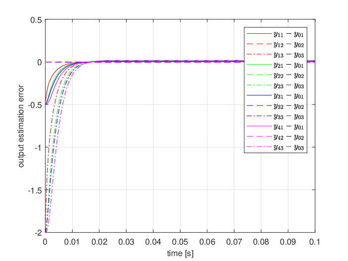
The communication graph $\bar{\mathcal{G}}$ is shown in Fig. 1. The gains of the output based adaptive distributed output observer are given as $\mu_{\alpha}=10$ , $\mu_{\zeta}=200$ . We let $a_{ij}=1$ whenever $(j,i)\in\bar{\mathcal{E}}$ . The elements of $\alpha_{i}(0)$ and $\zeta_{i}(0)$ for $i=1,2,3,4$ are taken from $[-1,1]$ . Fig. 2 shows the output estimation errors of the output based adaptive distributed observers.

It is interesting to make a comparison between the dimension of the output based adaptive distributed output observer (10), (13) and the dimension of the state based adaptive distributed output observer (4). In fact, simple calculation shows that the dimension of the state based adaptive distributed output observer (4) is 45 (25 for estimating $S_{0}\in\mathbb{R}^{5\times 5}$ , 15 for estimating $C_{0}\in\mathbb{R}^{3\times 5}$ , and 5 for estimating $v_{0}\in\mathbb{R}^{5}$ ) while the dimension of the output based adaptive distributed output observer (10), (13) is 20 (5 for estimating $\alpha_{0}\in\mathbb{R}^{5}$ and 15 for estimating $\zeta_{0}\in\mathbb{R}^{15}$ ). The comparisons between the dimensions as well as the information exchanges of the two observers are summarized in Table 1.

Table 1: Comparison between state based adaptive distributed output observer and output based adaptive distributed output observer (SB: state based; OB: output based).

control law dimension

information exchange

$S_{i}\in\mathbb{R}^{5\times 5}$	25
$C_{i}\in\mathbb{R}^{3\times 5}$	15
$v_{i}\in\mathbb{R}^{5}$	5
total	45

$S_{i}\in\mathbb{R}^{5\times 5}$	25
$C_{i}\in\mathbb{R}^{3\times 5}$	15
$v_{i}\in\mathbb{R}^{5}$	5
total	45

$\alpha_{i}\in\mathbb{R}^{5}$	5
$\zeta_{i}\in\mathbb{R}^{15}$	15
total	20

$\alpha_{i}\in\mathbb{R}^{5}$	5
$y_{i}\in\mathbb{R}^{3}$	3
total	8

Refer to caption — Figure 1: Communication network $\bar{\mathcal{G}}$ .

5 Conclusion

In this communique, we have proposed an output based adaptive distributed output observer. In contrast to the existing state based adaptive distributed output observers, the proposed output based adaptive distributed output observer only needs to know the output of the leader system. In addition, the dimension as well as the information exchange among agents of the output based adaptive distributed output observer can be significantly reduced in comparison with the state based adaptive distributed output observer.

References

[1] H. Cai and J. Huang,“The attitude consensus problem via an output based adaptive distributed observer approach,” Proceedings of the 2018 13th World Congress on Intelligent Control and Automation, July 4-8, 2018, Changsha, China, 2018.
[2] H. Cai, F. L. Lewis, G. Hu and J. Huang, “The adaptive distributed observer approach to the cooperative output regulation of linear multiagent systems”, Automatica, vol. 75, pp. 299-305, 2017.
[3] Z. Chen, “Pattern synchronization of nonlinear heterogeneous multiagent networks with jointly connected topologies”, IEEE Transactions on Control of Network Systems, vol. 1, no. 4, pp. 349-359, 2014.
[4] Z. Feng, G. Hu, W. Ren, W. E. Dixon and J. Mei, “Distributed coordination of multiple unknown Euler-Lagrange Systems”, IEEE Transactions on Control of Network Systems, vol. 5, no. 1, pp. 55-66, 2018.
[5] R. Horn and C. Johnson, Topics in Matrix Analysis, Cambridge University Press, 1991.
[6] J. Hu and Y. Hong, “Leader-following coordination of multiagent systems with coupling time delays,” Physica A: Statistical Mechanics and its Applications, vol. 374, no. 2, pp. 853–863, 2007.
[7] Y. Hua, X. Dong, Q. Li and Z. Ren, “Distributed adaptive formation tracking for heterogeneous multiagent systems with multiple nonidentical leaders and without well-informed follower”, International Journal of Robust and Nonlinear Control, vol. 30, pp. 2131-2151, 2020.
[8] A. Jadbabaie, J. Lin, and A. S. Morse, “Coordination of groups of mobile agents using nearest neighbor rules,” IEEE Transactions on Automatic Control, vol 48, no. 6, pp. 988-1001, Jun. 2003.
[9] S. Knorn, Z. Chen, R. Middleton, “Overview: collective control of multiagent systems,” IEEE Transactions on Control of Network Systems, vol 3, no. 4, pp. 334-347, Jun. 2016.
[10] P. Lancaster, L. Rodman, Algebraic Riccati equations, Oxford University Press, 1995.
[11] F. L. Lewis, H. Zhang, K. Hengster-Movric, A. Das, Cooperative Control of Multi-Agent Systems: Optimal and Adaptive Design Approacheds, Springer-Verlag: London, UK, 2014.
[12] H. Liang, Y. Zhou, H. Ma and Q. Zhou, “Adaptive distributed observer approach for cooperative containment control of nonidentical networks”, IEEE Transactions on Systems, Man, and Cybernetics: Systems, vol. 49, no. 2, pp. 299-307, 2019.
[13] R. Olfati-Saber, R. M. Murray, “Consensus problems in networks of agents with switching topology and time-delays”, IEEE Transactions on Automatic Control, vol. 49, no. 9, pp. 1520-1533, 2004.
[14] Z. Qu, Cooperative Control of Dynamical Systems: Applications to Autonomous Vehicles. Springer-Verlag: London, U.K., 2009.
[15] W. Ren, R. W. Beard, Distributed Consensus in Multi-Vehicle Cooperative Control, Communications and Control Engineering Series. Springer-Verlag: London, U.K., 2008.
[16] E. D. Sontag, “On the input-to-state stability property”, European Journal of Control, vol. 1, pp. 24-36, 1995.
[17] E. D. Sontag and Y. Wang, “New characterizations of input-to-state stability property”, IEEE Transactions on Automatic Control, vol. 41, pp. 1283-1294, 1996.
[18] Y. Su and J. Huang, “Cooperative output regulation of linear multiagent systems”, IEEE Transactions on Automatic Control, vol. 57, no. 4, pp. 1062-1066, 2012.
[19] Y. Su, Y. Hong, and J. Huang, “A general result on the cooperative robust output regulation for linear uncertain multiagent systems,” IEEE Transactions on Automatic Control, vol. 58, no. 5, pp. 1275-1279, May 2013.

Output Based Adaptive Distributed Output Observer for Leader-follower Multiagent Systemsfootnoteinfo