Adiabatic pumping driven by moving kink and quantum standard ampere in buckled graphene nanoribbon

Our analysis starts from the Su-Schrieffer-Heeger (SSH) Hamiltonian for graphene nanostructures Dre98; Kar17; Gro18, with potential energy describing the covalent bonds Tsa10

where

with a constrain

The kinetic-energy operator for $\pi$ electrons $T$ (2) includes the hopping-matrix elements ($t_{ij}$) corresponding to the nearest-neighbors on a honeycomb lattice (denoted by using brackets $\langle{ij}\rangle$), with the equilibrium hopping integral $t_{0}=2.7\,$eV. The change in bond length, $\delta{}d_{ij}=d_{ij}-d_{0}$, is calculated with respect to the equilibrium bond length $d_{0}=a/\sqrt{3}$, with $a=2.46\,$Å  being the lattice spacing. The operator $c_{i,s}^{\dagger}{}$ (or $c_{i,s}$) creates (or annihilates) a $\pi$ electron at the $i$-th lattice site with spin $s$. The electron-phonon coupling, quantified by the dimensionless parameter $\beta=-\left.\partial{}\ln{}t_{ij}/\partial\ln{}d_{ij}\right|_{d_{ij}=d_{0}}$ (to be specified later), is represented by the exponential factor in Eq. (2) replacing standard Peierls form $(1-\beta\delta{}d_{ij}/d_{0})$ in order to prevent $t_{ij}$ from changing the sign upon strong lattice deformation.

The next two terms in Eq. (1), $V_{\rm bond}$ (3) and $V_{\rm angles}$ (4), approximates the potential energies for the bond stretching and bond angle bending (respectively); see Fig. 2. The parameters $K_{d}=40.67\,$eV$/$Ų, $K_{\theta}=5.46\,$eV$/$rad², and $\theta_{0}=\pi/3$, are taken from Ref. Tsa10 and restore the actual in-plane elastic coefficients of bulk graphene in the case of $\beta=0$. Otherwise (for $\beta\neq{}0$), a correction to the potential energy per bond can be estimated as

with the number of C-C bonds $N_{b}$. The second approximate equality in the above is obtained by substituting $\sum_{s}\left\langle{}c_{i,s}^{\dagger}{}c_{j,s}+c_{j,s}^{\dagger}{}c_{i,s}\right\rangle\approx{}1.050$ (with $i$ and $j$ the nearest neighbors), being the value for a perfect, bulk graphene sheet at the half electronic filling Mar97foo.

The expression for $V_{\rm angles}$ (4) consists of two terms, each involving summation over the three angles $\measuredangle(j)$ having a common vertex at a given lattice site $j$ (see Fig. 2). First term, $\propto{}K_{\theta}$, represents the harmonic approximation for in-plane bond angle bending. For out-of plane deformations, quantified by the height $h_{j}$ of a tetrahedron formed by $j$-th site and its three nearest neighbors, this term represents a fourth-order correction to the potential energy. A realistic description of out-of-plane deformations requires a correction of the $\sim{}h_{j}^{2}$ order (for $h_{j}\ll{}d_{0}$). Here we propose a term proportional to the excess angle,

with the coefficient $V_{\delta}\approx{}t_{0}=2.7\,$eV roughly approximating the bending rigidity of graphene Der18; Voz10. The main advantage of such an approach is that it requires no computationally expensive operations since the four-body term ($\propto{}V_{\delta}$) depends only on angles ($\theta_{\measuredangle(j)}$) earlier determined for the three-body term ($\propto{}K_{\theta}$). The validity of our approach, in comparison with standard molecular dynamics treatments Yam17; Yam19, is discussed later in this paper.

Throughout the paper, we compare the results obtained in the absence of electron phonon coupling, $\beta=0$, and for the dimensionless parameter $\beta=3$; the two values chosen to bound the possible range of $\beta$ (see Ref. Voz10). It is worth to stress here that in the fortcoming analysis physical properties are discused as functions of the deformation applied, and thus the other choice of $\beta\neq{}0$ (being the propotionality coefficient between the local deformation and corresponding correction to the Hamiltonian) may rather shift the characteristic features observed than change the picture in a qualitative manner.

In the $\beta=0$, electronic and lattice degrees of freedom are decoupled, and one simply need to solve a purely classical minimization problem for the potential energy part of the Hamiltonian ${\cal H}_{\rm SSH}$ (1), given by $V_{\rm bonds}+V_{\rm angles}$ [see Eqs. (3) and (4)]. For the $\beta\neq{}0$ case, the average kinetic energy can be calculated as

where the factor $2$ in the last two expressions follows from a spin degeneracy, $t_{ij}=-t_{0}\exp(-\beta{}\delta{}d_{ij}/d_{0})$ if $i$ and $j$ are the nearest neighbors (otherwise, $t_{ij}=0$), and $\psi_{k}^{(j)}$ denotes the probability amplitude for the $k$-th eigenstate of the kinetic energy operator $T$ (2) at $j$-th lattice site. We further suppose that the eigenstates are ordered such that the energies $E_{1}\leqslant{}E_{2}\leqslant{}\dots\leqslant{}E_{N_{\rm at}}$, with the number of atoms $N_{\rm at}$, and that the number of electrons $N_{\rm el}$ is even for simplicity.

In both cases ($\beta=0$ and $\beta=3$), the numerical minimization of the ground-state energy

with respect to atomic positions $\{{\bf R}_{j}\}$, is performed employing the modified periodic boundary conditions in $y$-direction (see Fig. 1). Namely, the system is invariant upon $y\mapsto{}y+L$ and $z\mapsto{}-z$, forcing the kink formation in a buckled ribbon. The outermost two rows of atoms near each armchair edge are fixed during the minimization (see Fig. 2), and buckling of the ribbon is realized by changing the distance between the fixed edges [see Fig. 2(a)] from $W$ to $W^{\prime}<W$. Furthermore, the number of electrons is fixed at $N_{\rm el}=N_{\rm at}$, with $N_{\rm at}=3600$ for metallic armchair ribbon ($W=10\,a$, $L=90\sqrt{3}\,a$) or $N_{\rm at}=3960$ for insulating armchair ribbon ($W=11\,a$, $L=90\sqrt{3}\,a$). Although in open system, coupled to the leads, the average $N_{\rm el}$ varies with the chemical potential, such fluctuations (typically, limited to $\Delta\mu<0.1\,$eV or, equivalently, $\Delta{}N_{\rm el}/N_{\rm at}\approx{}0.18\,(\Delta{}\mu/t_{0})^{2}<2\times{}10^{-4}$; see Ref. Ryc16) are insignificant when determining the optimal bond lengths. Alternatively, one can interpret the $\beta=0$ case as a hypothetical $N_{\rm el}=0$ situation, leading to bond length modifications not exceeding a few percents (see below).

For a fixed $W^{\prime}/W$ ratio and the kink position $y=y_{0}$, the computations proceed as follows.

The initial arrangement of carbon atoms is given by

where

with $(\tilde{x}_{j},\tilde{y}_{j})$ being the coordinates of $j$-th atom on a flat honeycomb lattice, and the scaling function

The buckle height $H$ in Eq. (11) is adjusted such that ${\cal C}=N_{\rm b}d_{0}$ in Eq. (5). The kink size is fixed at $\Lambda=5\,a$, roughly approximating the kink profiles reported in Refs. Yam17; Yam19.

At first step, we minimize the potential energy term $V_{\rm bonds}+V_{\rm angles}$, ignoring a constrain given by Eq. (5). This gives us the solution for $\beta=0$ in the Hamiltonian ${\cal H}_{\rm SSH}$ (1).

Next step, performed only if $\beta>0$, involves a further adjustment of atomic positions $\{{\bf R}_{j}\}$ such that full ground-state energy $E_{G}$ (9) reaches a minimum. In practice, we determine hopping parameters $\{t_{ij}\}$, wavefunctions $\left\{\psi_{k}^{(j)}\right\}$, and correlation functions $\left\{\langle{}c_{is}^{\dagger}c_{js}\rangle\right\}$ [see Eq. (8)] for given $\{{\bf R}_{j}\}$-s, and then find (within the gradient descent method) a conditional minimum of $E_{G}$ with respect to $\{{\bf R}_{j}\}$ at fixed values of $\left\{\langle{}c_{is}^{\dagger}c_{js}\rangle\right\}$-s, satisfying a constrain given by Eq. (5). The procedure is iterated until the numerical convergence is reached. Typically, after $3$–$4$ iterations the atomic positions $\{{\bf R}_{j}\}$-s are determined with the accuracy better then $10^{-5}\,a$.

A brief comparison of the kink shape following from the numerical procedure described above with the corresponding output produced by the LAMMPS Molecular Dynamics Simulator Pli95; lamm2 is presented in Fig. 3.

In order to quantify the difference in atomic arrangements obtained within different approaches, we choose the maximal absolute displacement of atom along the $x$ (and $y$) axis, max$\,|x-x^{(0)}|$ (and max$\,|y-y^{(0)}|$), where the maximum is taken for a subset of atoms with equal initial $y^{(0)}$ coordinates; see Figs. 3(a) and 3(b). It is sufficient to display the data corresponding to a vicinity of the kink, $30\leqslant{}y^{(0)}/a\leqslant{}90$, since far away from the kink position (being fixed at $y_{0}\approx{}58.5\,a$) both the quantities considered become $y^{(0)}$-independent. (As free boundary conditions are applied in case the LAMMPS package is utilized, some $y^{(0)}$-dependences reappear near the free zigzag edges, but they are much smaller in magnitude than dependencies in the kink area.)

It is clear from Figs. 3(a) and 3(b) that the LAMMPS results (see red-dashed lines) are closer to the obtained with our optimization procedure in the presence of electron-phonon coupling, $\beta=3$ (solid symbols), then for $\beta=0$ (open symbols). Also, $x$–$z$ views of the system, presented in Figs. 3(c), 3(d), and 3(e), show that approximate mirror symmetry of the kink appears for $\beta=3$ [see Fig. 3(d)] and for the LAMMPS results [Fig. 3(e)], but is absent for $\beta=0$ [Fig. 3(c)].

The above observations can be rationalized taking into accout that four-body (dihedral) and long-range Lennard-Jones potential energy terms are included in the LAMMPS package but absent in our model Hamiltonian ${\cal H}_{\rm SSH}$ (1). In the presence of electron-phonon coupling ($\beta>0$), however, the average kinetic energy $\langle{}T\rangle$ (8) can be interpreted as an effective long-range (and “infinite-body”) attractive interaction between atoms, restoring some features related to the Lennard-Jones forces in molecular dynamics (including an approximate mirror symmetry of the kink).

Before discussing the electronic structure of the system, we briefly describe small corrections to the bond lengths appearing in the kink area due to electron-phonon coupling (see Fig. 4), which are essential to understand the results presented in the remaining parts of the paper.

In Figs. 4(a) and 4(b) we visualize the spatial arrangements of shorten and lengthen bonds; namely, $d_{ij}<\langle{}d_{ij}\rangle{}_{i,j=1\dots{}N_{\rm at}}$ (thick black lines) and $d_{ij}>\langle{}d_{ij}\rangle{}$ (thin red lines), where the average bond length $\langle{}d_{ij}\rangle{}=0.998\,d_{0}$ for $\beta=0$ and $W^{\prime}/W=0.9$, or $\langle{}d_{ij}\rangle{}\equiv{}d_{0}$ for $\beta=3$ due to a constrain imposed [see Eq. (5)]. Apparently, in the presence of electron-phonon coupling ($\beta=3$) a large rectangular block is formed in the kink area [i.e., for $|y-y_{0}|\lesssim{}7\,a$; see Fig. 4(b)], in which almost all bonds oriented in the zigzag direction are shorten (resulting in the hopping element $|t_{ij}|>t_{0}$) and almost all remaining bonds are lengthen ($|t_{ij}|<t_{0}$). In the absence of electron-phonon coupling ($\beta=0$) the situation is less clear [Fig. 4(a)], with a few smaller blocks of shorten or lengthen bonds forming more complex patterns, some of which are isotropic, and some show various crystallographic orientations.

The qualitative finding presented above is further supported with statistical distributions of the relative bond length ($d_{ij}/d_{0}$), determined using all $N_{\rm b}=5749$ bonds in the system (for $L=90\sqrt{3}\,a$ and $W=11\,a$) and displayed in Figs. 4(c) and 4(d). In particular, the distribution for $\beta=3$ [Fig. 4(d)] is significantly wider than for $\beta=0$ [Fig. 4(c)]. Also, bimodal structure of the distribution is visible in the presence of electron-phonon coupling, suggesting that two distinct populations of shorten and lengthen bonds are formed in this case.

The position dependence of the bond-length modulation is illustrated in Figs. 4(e) and 4(f), where we display the mean $\langle{}d_{ij}\rangle{}$ the variance Var$\,(d_{ij})$ calculated for bonds connecting atoms in a single zigzag line (parallel to the $x$ direction) as functions of a mean $y$-position of carbon atoms in the line. It is clear that significant bond-length modulations (however, not exceeding a few percents of $d_{0}$) appear only in a small vicinity of the kink position, $|y-y_{0}|\lesssim{}7\,a$, and that the modulations and noticeably stronger for $\beta=3$ (solid symbols) than for $\beta=0$ (open symbols). Remarkably, the LAMMPS results (red-dashed lines) now indicate much weaker bond-length modulations than our numerical results (regardless $\beta=0$ or $\beta=3$) but are significantly closer to the $\beta=0$ results then to the $\beta=3$ results. This shows that the quantum-mechanical nature of the Hamiltonian ${\cal H}_{\rm SSH}$ (1), relevant for spacial arrangement of carbon atoms only if $\beta\neq{}0$, is crucial for an accurate description of bond-lengths corrections.

In order to understand how the bond-length modulation may affect the transport properties, we focus now on the Dirac points ($K$ and $K^{\prime}$) and changes in their positions in the first Brillouin zone due to strain-induced fields (see Fig. 5).

Revisiting the derivation of an effective Dirac equation for graphene one finds that weak deformations introduce peculiar gauge fields, with the vector potential for $K$ valley Voz10

where $c$ is a dimensionless coefficient of the order of unity, $u_{ij}=\frac{1}{2}(\partial_{i}{}u_{j}+\partial_{j}{}u_{i})$ (with $i,j=x,y$) is the symmetrized strain tensor for in-plane deformations Lan59 and the coordinate system is chosen as in Fig. 1 (i.e., such that the $x$ axis corresponds to a zigzag direction of a honeycomb lattice). For the $K^{\prime}$ valley, the strain-induced field has an opposite sign (namely, ${\mbox{\boldmath${A}$}}_{K^{\prime}}=-{\mbox{\boldmath${A}$}}_{K}$).

For an approximately uniform compression along the $x$ direction occurring in the kink area, we have $u_{x}\approx{}(W^{\prime}/W)x$, $u_{y}=y$, and the $K$ point is shift by $\delta{}\mbox{\boldmath${A}$}\propto{}-(1-W^{\prime}/W)\hat{k}_{x}$ with $\hat{k}_{x}$ being a unit vector in the $k_{x}$ direction, while the $K^{\prime}$ point is shift by $-\delta\mbox{\boldmath${A}$}$, as visualized in top panels of Fig. 5. Away from the kink area, buckling without changing bond lengths does not create strain-induced fields ($\delta{\mbox{\boldmath${A}$}}\approx{}0$) scalarfoo.

Additionally, a finite size along the $x$ direction introduces the well-known geometric quantization, with the discrete values of quasimomentum $k_{x}$, separated by $\Delta{}k_{x}\sim{}\pi/W$ (see bottom panels in Fig. 5). In principle, for a particular combination of $\delta\mbox{\boldmath${A}$}$ and $\Delta{}k_{x}$, a nanoribbon may locally change its character from metallic to insulating (or vice versa). In more general situation, if $\delta\mbox{\boldmath${A}$}$ and $\Delta{}k_{x}$ are not precisely adjusted to alter the system properties at $E=0$, one can find some finite energies ($E>0$ for electrons or $E<0$ for holes), for which quantum states are available only away from the kink area (or only in the kink area). A direct illustration is provided with the density of states discussed next.

We consider here two nanoribbons with armchair edges, one of the width $W=10\,a$ (the metallic case) and the other of $W=11\,a$ (the insulating case). The system length is $L=90\sqrt{3}\,a$ in both cases, with modified periodic boundary conditions (see Sec. II.2) applied for both lattice and electronic degrees of freedom. The two values of $\beta=0$ and $\beta=3$ in the Hamiltonian ${\cal H}_{\rm SSH}$ (1) are considered; the buckling magnitude is fixed at $W^{\prime}/W=0.9$. The above parameters allow us to define the two energy scales: The subband splitting

and the longitudinal quantization

In Fig. 6, we display the electronic density of states

with $E_{n}$ denoting the $n$-th eigenvalue of the kinetic-energy operator $T$ given by Eq. (2), for all four combinations of $\beta$ and $W$. For plotting purposes, the $\delta$ function is smeared by a finite $\epsilon$; namely, we put

where $\epsilon=5\cdot{}10^{-3}\,t_{0}$.

Since $\Delta{}E_{W}\gg{}\Delta{}E_{L}$, metallic [see Figs. 6(a) and 6(b)] or insulating [see Figs. 6(c) and 6(d)] character of the ribbon can still be recognized from the $\rho(E)$ spectrum of its finite section: in the former case, $\rho(E)$ is elevated for any $E$, whereas in the later case, we have $\rho(E)\approx{}0$ in a vicinity of $E=0$.

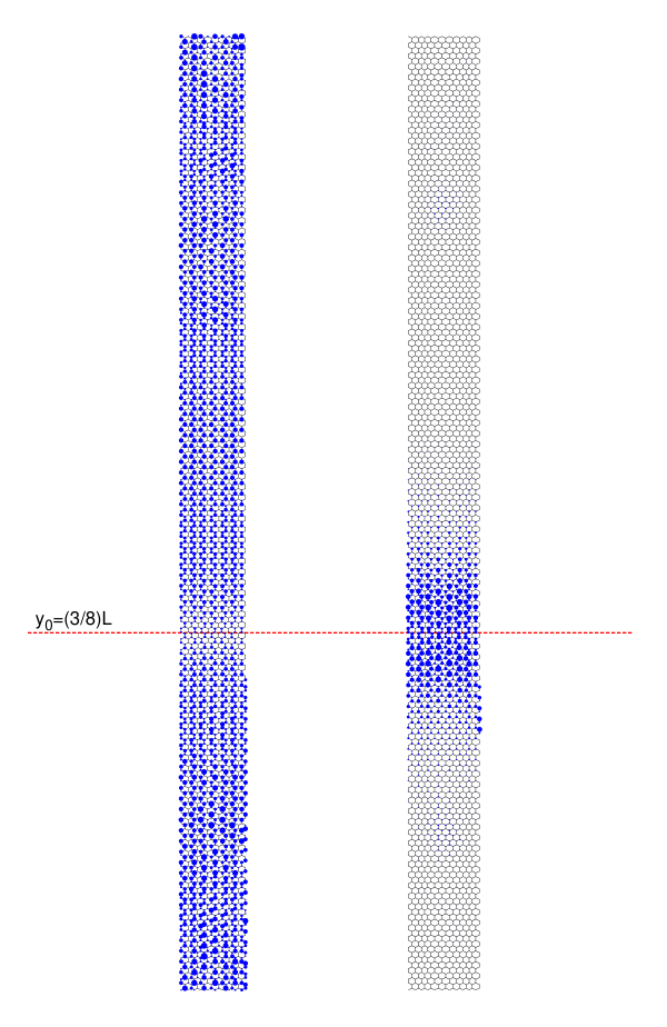
The effects of electron-phonon coupling can be summarized as follows. In the metallic case, bond length modulation results in small splittings of the electronic levels [see Fig. 6(b) for $\beta=3$], originally showing approximate degeneracy [see Fig. 6(a) for $\beta=0$], due to amplified scattering between the $k_{y}$ and $-k_{y}$ states occurring in the kink area. In the insulating case, we have two energy levels, appearing for $\beta=3$ [see Fig. 6(d)] but absent for $\beta=0$ [see Fig. 6(c)], one for electrons (marked with red arrow) and one for holes, which occur in the gap range and are well-separated from other levels, suggesting that they are associated with localized states.

The above expectation is further supported with local density of states (presented Fig. 7)

where the $\delta$ function is represented via Eq. (17) and the remaining symbols are same as in Eq. (8). Adjusting the energy to the isolated electronic level appearing in the insulating case ($W=11\,a$) at $E=0.04\,t_{0}$, we immediately find that the corresponding quantum state is strongly localized in the kink area (see right panel in Fig. 7). In the metallic case ($W=10\,a$), the value of $E=0.04\,t_{0}$ belongs to a continuum of extended states in the lowest subband, but the corresponding $\rho_{\rm loc}({\bf R}_{j},E)$ profile shows a clear suppression in the kink area (see left panel in Fig. 7), allowing one to expect that the current propagation in $y$-direction may be blocked, in the presence of a kink, for a whole energy window corresponding to the lowest (or highest) subband for electron (or holes).

So far, we have discussed several characteristics of the closed system with modified periodic boundary conditions in the $y$-direction (see Sec. III), making the kink position ($y_{0}$) irrelevant for global characteristics, such as the density of states. Now, we use the atomic positions $\{{\bf R}_{j}\}=\{(x_{j},y_{j},z_{j})\}$ obtained with the optimization procedure described in Sec. II.2 (again, we consider the cases without and with the electron-phonon coupling, $\beta=0$ and $\beta=3$) for $y_{0}=\frac{3}{8}L$. Next, the kink is placed at the desired position (say, $y_{0}+\Delta{}y$) by applying a shift to all $y$ coordinates, $y\mapsto{}y+\Delta{}y$. A series of consequitive shifts, such as visualized in Fig. 8, emulates the kink motion (including full kink and antikink transitions) in a real system. In case the shift is commensurate with the longitudinal ribbon periodicity, $\Delta{}y=\sqrt{3}na$ with $n$-integer, we simply apply modified periodic boundary conditions for all atoms, for which $y_{j}+\Delta{}y<0$ or $y_{j}+\Delta{}y\geqslant{}0$. Otherwise (i.e., if $\Delta{}y\neq{}na$), atomic positions after a shift $\{{\bf R}_{j}\}_{\Delta{}y}$ are determined via third-order spline interpolation using $\{{\bf R}_{j}\}_{\sqrt{3}(n_{0}-1)a}$, $\{{\bf R}_{j}\}_{\sqrt{3}n_{0}a}$, …, $\{{\bf R}_{j}\}_{\sqrt{3}(n_{0}+2)a}$, with $n_{0}=\lfloor\Delta{}y/(\sqrt{3}a)\rfloor$, and $\lfloor{}x\rfloor$ the foor function of $x$.

The hopping-matrix elements ($t_{ij}$) in Eq. (8) are then determined using atomic positions after a shift, $\{{\bf R}_{j}\}_{\Delta{}y}$, but we set $t_{ij}=0$ in case $i$ and $j$ are terminal atoms from the opposite zigzag edges (i.e., periodic boundary conditions are no longer applied for electronic degrees of freedom).

The leads, positioned at the areas of $x<0$ and $x>W^{\prime}$ in Fig. 1, are modeled as perfectly flat (i.e., $t_{ij}=-t_{0}$ for the nearest neighbors $i$ and $j$) and heavily doped graphene areas, with the electrostatic potential energy $U_{\infty}=-0.5\,t_{0}$ (compared to $U_{0}=0$ in the ribbon area, $0<x<W^{\prime}$), each of the width $W_{\infty}=17.5\sqrt{3}\,a$ (corresponding to $11$ propagating modes for $E=0$). What is more, both leads are offset from the free ribbon edges by a distance of $L_{s}=7.5\sqrt{3}\,a$, suppressing the boundary effects. The scattering problem is solved numerically, for each value of the chemical potential $\mu=E-U_{0}$ and the kink position $y_{0}$, using the Kwant package Kwant in order to determine the scattering matrix

which contains the transmission $t\,$ ($t^{\prime}$) and reflection $r\,$ ($r^{\prime}$) amplitudes for charge carriers incident from left (right) lead.

The linear-response conductance is determined from the $S$-matrix via the Landauer-Büttiker formula Lan57; But85, namely

where $G_{0}=2e^{2}/h$ is the conductance quantum and $T_{n}$ is the transmission probability for the $n$-th normal mode.

In Fig. 9, we compare the conductance spectra for the same four combinations of parameters $W$ and $\beta$ as earlier used when discussing the density of states (see Fig. 6). This time, results for a buckled ribbon, with $W^{\prime}/W=0.9$ and a kink placed at $y_{0}=\frac{3}{8}L$, are compared with the corresponding results for a flat ribbon (solid blue and dashed red lines in Fig. 9, respectively). In the metallic case, electron-phonon coupling strongly suppresses the transport in the presence of a kink [Fig. 9(b)]; the effect of a kink is much weaker in the absence of electron-phonon coupling [Fig. 9(a)]. Similar effects can be noticed in the insulating case, provided that the chemical potential is adjusted to the first conductance step above (or below) the gap range [Figs. 9(c) and 9(d)].

In the absence of a voltage bias between the leads, the charge transferred solely due to adiabatic kink motion (i.e., by varying the parameter $y_{0}$) can be written as Naz09

where the summation runs over the modes in a selected (output) lead. We further notice that molecular dynamics simulations of Refs. Yam17; Yam19 allow to estimate typical kink velocity (up to the order of magnitude) as $v_{\rm kink}\sim{}1\,$km/s$\ \ll{}v_{F}$, where $v_{F}=\sqrt{3}\,t_{0}{}a/(2\hbar)\approx{}10^{6}\,$m/s is the Fermi velocity in graphene, justifying the adiabatic approximation ekinkfoo.

Numerical results for $\Delta{}Q(\mu)$, obtained by shifting the kink from $y_{0}=0$ to $y_{0}=L$, are presented in Fig. 10. Although the current blocking in the metallic case is far from being perfect [see Fig. 9(b)], the related pumping mechanism for $W=10\,a$ appears to be rather effective (see top panel in Fig. 10), with $\Delta{}Q(\mu)$ approaching the total charge available for transfer in a section of the length $L_{\rm eff}$, a value of which can be approximated by qkinkfoo

where we put $L_{1}\leqslant{}L_{\rm eff}\leqslant{}L_{1}+W_{\infty}$ estimating the effective length of a ribbon section between the leads (see shaded area in Fig. 10).

Significant changes to the $\Delta{}Q(\mu)$ spectra are observed in the insulating case of $W=11\,a$ (see bottom panel in Fig. 10). Namely, there is an abrupt switching between $\Delta{}Q\approx{}0$ near the center of a gap (at $\mu=0$) and $\Delta{}Q\approx{}2e$ appearing for $\mu$ exceeding the energy level localized in the kink area [see Fig. 6(d)]. The value of $\Delta{}Q\approx{}2e$ remains unaffected until $\mu$ approaches a bottom of the lowest electronic subband [corresponding to the first conductance step in Fig. 9(d)]. For higher $\mu$, the picture becomes qualitatively similar to this for a metalic case, with $\Delta{}Q(\mu)$ systematically growing with $\mu$ and degreasing with $W^{\prime}/W$. Noticeably, the plateau with $\Delta{}Q\approx{}2e$ is well-developed starting from moderate bucklings, $W^{\prime}/W\approx{}0.95$. For $W^{\prime}/W\approx{}0.9$, deviation from the quantum value in the plateau range is of the order of $|\Delta{}Q-2e|\sim{}10^{-4}\,e$, and can be attributed to the finite-size effects. Some stronger deviations may appear in a more realistic situation due to the finite-temperature and non-adiabatic effects, which are beyond the scope of this work.

In both (metallic and insulating) cases, the stability of numerical integration in Eq. (21) substantially improves for the lead offsets $L_{s}\gtrsim{}5\,a$ (being comparable with the kink size), for which parts of the ribbon attached to the leads, together with a section between the leads, are (almost) uniformly buckled for either $y_{0}\approx{}0$ or $y_{0}\approx{}L$.

In Fig. 10, we also display maximal bond distortions for different bucklings (see the inset), showing that local deformations $|\delta{}d_{ij}|<0.1\,d_{0}$ for all $0.9\leqslant{}W^{\prime}/W<1$.

References

- (1) M. M. Benameur, F. Gargiulo, S. Manzeli, G. Autés, M. Tosun, O. V. Yazyev, and A. Kis, Nat. Commun. 6, 8582 (2015).
- (2) Z. H. Khan, A. R. Kermany, and F. Iacopi, J. Phys. D: Appl. Phys. 50, 053003 (2017).
- (3) M. I. Katsnelson, Graphene: Carbon in Two Dimensions, (Cambridge University Press, Cambridge, 2012), Chapter 1.
- (4) J.-L. Tsai and J.-F. Tu, Mater. Des. 31, 194 (2010).
- (5) A. Derras-Chouk, E. M. Chudnovsky, D. A. Garanin, and R. Jaafar, J. Phys. D: Appl. Phys. 51, 195301 (2018).
- (6) M. A. H. Vozmediano, M. I. Katsnelson, and F. Guinea, Phys. Rep. 496, 109 (2010).
- (7) E. Prada, P. San-Jose, and H. Schomerus, Solid State Comm. 151, 1065 (2011).
- (8) M. Wakker and M. Blaauboer, Phys. Rev. B 82, 205432 (2010).
- (9) P. San-Jose, E. Prada, H. Schomerus, and S. Kohler, Appl. Phys. Lett. 101, 153506 (2012).
- (10) Y. Jiang, T. Low, K. Chang, M. I. Katsnelson, and F. Guinea, Phys. Rev. Lett. 110, 046601 (2013).
- (11) E. Grichuk and E. Manykin, Eur. Phys. J. B 86, 210 (2013).
- (12) B. Abdollahipour and E. Moomivand, Physica E 86 204 (2017).
- (13) M. Fujimoto, H. Koschke, and M. Koshino, Phys. Rev. B 101, 041112 (2020).
- (14) Y. Zhang, Y. Gao, and D. Xiao, Phys. Rev. B 101, 041410(R) (2020)
- (15) D. Suszalski and A. Rycerz, e-print arXiv:2002.08507 (unpublished).
- (16) Yu. V. Nazarov and Ya. M. Blanter, Quantum Transport: Introduction to Nanoscience, (Cambridge University Press, Cambridge, 2009), Chapter 1.
- (17) J. P. Pekola, O. P. Saira, V. Maisi, A. Kemppinen, M. Möttönen, Y. A. Pashkin, and D. Averin, Rev. Mod. Phys. 85, 1421 (2013).
- (18) N.-H. Kaneko, S. Nakamura, and Y. Okazaki, Meas. Sci. Technol. 27, 032001 (2016).
- (19) W. Poirier, S. Djordjevic, F. Schopfer, and O. Thévenot, C. R. Physique 20, 92 (2019).
- (20) D. B. Newell, F. Cabiati, J. Fischer, K. Fujii, S. G. Karshenboim, H. S. Margolis, E. de Mirandés, P. J. Mohr, F. Nez, K. Pachucki, T. J. Quinn, B. N. Taylor, M. Wang, B. M. Wood, and Z. Zhang, Metrologia 55, L13 (2018).
- (21) P. J. Mohr, B. D. Newell, B. N. Taylor, and E. Tiesinga, Metrologia 55, 125 (2018).
- (22) R. D. Yamaletdinov, V. A. Slipko, and Y. V. Pershin, Phys. Rev. B 96, 094306 (2017).
- (23) R. D. Yamaletdinov, T. Romańczukiewicz, and Y. V. Pershin, Carbon 141, 253 (2019).
- (24) G. Dresselhaus, M. S. Dresselhaus, and R. Saito, Physical Properties Of Carbon Nanotubes, (World Scientific, Singapore, 1998), Chapter 11.
- (25) R. Peierls, Quantum Theory of Solids, (Oxford University Press, Oxford 1955), Chapter V.
- (26) S. Plimpton, J. Comp. Phys. 117, 1 (1995); see also: http://lammps.sandia.gov.
- (27) Interactions between carbon atoms are described using the standard two-body, three-body, four-body (dihedral), and Lennard-Jones potential energy terms, see Ref. Yam17. Periodic boundary conditions in -direction are not applied in this case.
- (28) T. Kariyado and X. Hu, Sci. Rep. 7, 16515 (2017).
- (29) O. Gröning, S. Wang, X. Yao, et al., Nature 560, 209 (2018).
- (30) The corresponding value of kinetic energy per site is (with ); see e.g.: L. M. Martelo, M. Dzierzawa, L. Siffert, D. Baeriswyl, Z. Phys. B 103, 335 (1997).
- (31) A. Rycerz, in Recent Advances in Graphene Research, P. Nayak (ed.), InTech DOI:10.5772/64240 (2016) pp. 91-110; e-print arXiv:1604.03783.
- (32) L.D. Landau and E.M. Lifschitz, Theory of Elasticity (Pergamon Press, Oxford, 1959).
- (33) Some scalar fields, modifying the electrostatic potential energy by , may also appear in the kink area (see Ref. Voz10) but they are neglected in our analysis, since the coupling constant is not determined precisely (various works report eV); also, the effective electrostatic potential barrier cannot substantially alter the current blocking (or the electron trapping) mechanism due to Klein tunelling.
- (34) C. W. Groth, M. Wimmer, A. R. Akhmerov, and X. Waintal, New J. Phys. 16, 063065 (2014); see also: https://kwant-project.org.
- (35) R. Landauer, IBM J. Res. Dev. 1, 233 (1957).
- (36) M. Büttiker, Y. Imry, R. Landauer, and S. Pinhas, Phys. Rev. B 31 6207 (1985).
- (37) In particular, local electric-field variation due to kink transition can roughly be estimated as , with quantifying the transition time for a fixed position along the ribbon, and being the vector potential given by Eq. (13) in the main text. For the geometry considered, the potential energy variation is significant only in the direction and can be bounded by . For the strain amplitude and , one finds the ratio , with the subband splitting given by Eq. (14) in the main text.
- (38) Eq. (22) follows from the dispersion relation for lowest subbands in the metallic case (with opposite group velocities), ; the contribution from higher subbands may be suppressed due to mismatching group velocities.