跳到论文正文
W Papers独立论文阅读器 arXiv:2007.11093 论文正文 计算阅读时间 · 0%
引用这篇论文根据当前论文元数据生成,正式投稿前建议核对。


License: arXiv.org perpetual non-exclusive license
arXiv:2007.11093v1 [cs.DS] 21 Jul 2020

Improved lower and upper bounds on the tile complexity of uniquely self-assembling a thin rectangle non-cooperatively in 3D

David Furcy Thanks: Computer Science Department, University of Wisconsin Oshkosh, Oshkosh, WI 54901, USA,furcyd@uwosh.edu.    Scott M. Summers Thanks: Computer Science Department, University of Wisconsin Oshkosh, Oshkosh, WI 54901, USA,summerss@uwosh.edu.    Logan Withers Thanks: Computer Science Department, University of Wisconsin Oshkosh, Oshkosh, WI 54901, USA,withel75@uwosh.edu.
Abstract

We investigate a fundamental question regarding a benchmark class of shapes in one of the simplest, yet most widely utilized abstract models of algorithmic tile self-assembly. More specifically, we study the directed tile complexity of a k×Nk\times N thin rectangle in Winfree’s ubiquitous abstract Tile Assembly Model, assuming that cooperative binding cannot be enforced (temperature-1 self-assembly) and that tiles are allowed to be placed at most one step into the third dimension (just-barely 3D). While the directed tile complexities of a square and a scaled-up version of any algorithmically specified shape at temperature 1 in just-barely 3D are both asymptotically the same as they are (respectively) at temperature 2 in 2D, the (loose) bounds on the directed tile complexity of a thin rectangle at temperature 2 in 2D are not currently known to hold at temperature 1 in just-barely 3D. Motivated by this discrepancy, we establish new lower and upper bounds on the directed tile complexity of a thin rectangle at temperature 1 in just-barely 3D. On our way to proving our lower bound, we develop a new, more powerful type of specialized Window Movie Lemma that lets us derive our lower bound via a counting argument, where we upper bound the number of “sufficiently similar” ways to assign glues to a set (rather than a sequence) of fixed locations. Consequently, our lower bound, Ω⁡(N1k)\Omega\left(N^{\frac{1}{k}}\right), is an asymptotic improvement over the previous state of the art lower bound and is more aesthetically pleasing since it eliminates the non-constant term kk that used to divide N1kN^{\frac{1}{k}}. The proof of our upper bound is based on the construction of a novel, just-barely 3D temperature-1 counter, organized according to “digit regions”, which affords it roughly fifty percent more digits for the same target rectangle compared to the previous state of the art counter. This increase in digit density results in an upper bound of O⁡(N1⌊k2⌋+log⁡N)O\left(N^{\frac{1}{\left\lfloor\frac{k}{2}\right\rfloor}}+\log N\right), that is an asymptotic improvement over the previous state of the art upper bound and roughly the square of our lower bound.

1 Introduction

A key objective in algorithmic self-assembly is to characterize the extent to which an algorithm can be converted to an efficient self-assembling system comprised of discrete, distributed and disorganized units that, through random encounters with and locally-defined reactions to each other, coalesce into a terminal assembly having a desirable form or function. In this paper, we study a fundamental question regarding a benchmark class of shapes in one of the simplest yet most popular abstract models of algorithmic self-assembly.

Ubiquitous throughout the theory of algorithmic self-assembly, Erik Winfree’s abstract Tile Assembly Model (aTAM) [12] is a discrete mathematical model of DNA tile self-assembly [9] that augments classical Wang tiling [11] with a mechanism for automatic growth. In the aTAM, a DNA tile is represented by a unit square (or cube) tile type that may neither rotate, reflect, nor fold. Each side of a tile type is decorated with a glue consisting of both a non-negative integer strength and an alpha-numeric label. A tile set is a finite set of tile types, from which infinitely many tiles of each type may be instantiated. If one tile is positioned at an unoccupied location Manhattan distance 1 away from another tile and their opposing glues are equal, then the two tiles bind with the strength of the opposite glues. A special seed tile type is designated and a seed tile, which defines the seed-containing assembly, is placed at some fixed location. During the process of self-assembly, a sequence of tiles bind to and never detach from the seed-containing assembly, provided that each one, in a non-overlapping fashion, binds to one or more tiles in the seed-containing assembly with total strength at least a certain positive integer value called the temperature. If the temperature is greater than or equal to 2, then it is possible to enforce cooperative binding, where a tile may be prevented from binding at a certain location until at least two adjacent locations become occupied by tiles. Otherwise, only non-cooperative binding is allowed (temperature-1 self-assembly). A fundamental question regarding a given shape is determining the effect of the value of the temperature on its directed tile complexity, or the size of the smallest tile set that, regardless of the order in which tiles bind to the seed-containing assembly, always self-assembles into a unique terminal assembly of tiles that are placed on and only on points of the shape.

Although temperature-1 self-assembly cannot enforce cooperative binding, there is a striking resemblance of its computational and geometric expressiveness in just-barely 3D, where tiles are allowed to be placed at most one step in the third dimension, to that of temperature-2 self-assembly in 2D, with respect to the directed tile complexity of two benchmark shapes: a square and a scaled-up version of any algorithmically specified shape. Adleman, Cheng, Goel and Huang [1] proved, using optimal base conversion, that the directed tile complexity of an N×NN\times N square at temperature 2 in 2D is O⁡(log⁡Nlog⁡log⁡N)O\left(\frac{\log N}{\log\log N}\right), matching a corresponding lower bound for all Kolmogorov-random NN and all positive temperature values, set by Rothemund and Winfree [8]. Both of these bounds hold for temperature-1 self-assembly in just-barely 3D. The lower bound is an easy generalization of the latter and the upper bound was established by Furcy, Micka and Summers [4] via their discovery of a just-barely 3D, optimal encoding construction at temperature 1. Just-barely 3D, optimal encoding at temperature 1 was inspired by, achieves the same result as, but is drastically different from the 2D optimal encoding at temperature 2 developed by Soloveichik and Winfree [10], who proved that the directed tile complexity of a scaled-up version of any algorithmically specified shape XX at temperature 2 is Θ⁡(K⁡(X)log⁡K⁡(X))\Theta\left(\frac{K(X)}{\log K(X)}\right), where K⁡(X)K(X) is the size of the smallest Turing machine that outputs the list of points in XX. This tight bound for temperature-2 self-assembly in 2D was shown to hold for temperature-1 self-assembly in just-barely 3D by Furcy and Summers [5]: they combined just-barely 3D optimal encoding at temperature 1 with a modified version of a just-barely 3D, temperature-1 Turing machine simulation by Cook, Fu and Schweller [3].

Another benchmark shape is the k×Nk\times N rectangle, where k<log⁡Nlog⁡log⁡N−log⁡log⁡log⁡Nk<\frac{\log N}{\log\log N-\log\log\log N}, making it “thin”. A thin rectangle is an interesting testbed because its restricted height creates a limited channel through which tiles may propagate information, for example, the current value of a self-assembling counter. In fact, Aggarwal, Cheng, Goldwasser, Kao, Moisset de Espanés and Schweller [2] used an optimal, base-⌈N1k⌉\left\lceil N^{\frac{1}{k}}\right\rceil counter that uniquely self-assembles within the restricted confines of a thin rectangle to derive an upper bound of O⁡(N1k+k)O\left(N^{\frac{1}{k}}+k\right) on the directed tile complexity of a k×Nk\times N thin rectangle at temperature 2 in 2D. They then leveraged the limited bandwidth of a thin rectangle in a counting argument for a corresponding lower bound of Ω⁡(N1kk)\Omega\left(\frac{N^{\frac{1}{k}}}{k}\right). The previous theory for a square and an algorithmically specified shape would suggest that these thin rectangle bounds should hold at temperature 1 in just-barely 3D. Yet, we currently do not know if this is the case. Thus, the power of temperature-1 self-assembly in just-barely 3D resembles that of temperature-2 self-assembly in 2D, with respect to the directed tile complexities of a square and a scaled-up version of any algorithmically specified shape, but not a thin rectangle.

2D Temperature 2 Just-barely 3D Temperature 1
Lower bound Upper bound Lower bound Upper bound
N×NN\times N Square Θ⁡(log⁡Nlog⁡log⁡N)\Theta\left(\frac{\log N}{\log\log N}\right) Same as 2D Temperature 2
Algorithmically-defined shape XX Θ⁡(K⁡(X)log⁡K⁡(X))\Theta\left(\frac{K(X)}{\log K(X)}\right) Same as 2D Temperature 2
k×Nk\times N rectangle Ω⁡(N1kk)\Omega\left(\frac{N^{\frac{1}{k}}}{k}\right) O⁡(N1k+k)O\left(N^{\frac{1}{k}}+k\right) Ω⁡(N12​kk)\Omega\left(\frac{N^{\frac{1}{2k}}}{k}\right) O⁡(N1⌊k3⌋+log⁡N)O\left(N^{\frac{1}{\left\lfloor\frac{k}{3}\right\rfloor}}+\log N\right)
Table 1: State-of-the-art directed tile complexity for the self-assembly of benchmark shapes in the aTAM, where K⁡(X)K(X) is the size of the smallest Turing machine that outputs the list of points in XX.
2D Temperature 2 Just-barely 3D Temperature 1
Lower bound Upper bound Lower bound Upper bound
k×Nk\times N rectangle N/A N/A Ω⁡(N1k)\Omega\left(N^{\frac{1}{k}}\right) O⁡(N1⌊k2⌋+log⁡N)O\left(N^{\frac{1}{\left\lfloor\frac{k}{2}\right\rfloor}}+\log N\right)
Table 2: Our improved lower and upper bounds on the directed tile complexity of rectangles are highlighted in this table as the two main contributions of this paper. Note that, for a thin rectangle, the additive terms in this table and Table 1 are eliminated.

Motivated by this theoretical discrepancy, we prove new lower and upper bounds on the directed tile complexity of a thin rectangle at temperature 1 in just-barely 3D. See Tables 1 and 2 for a quick summary of our results and how they compare with previous state of the art results. Our lower bound is:

Theorem 1.

The directed tile complexity of a k×Nk\times N thin rectangle at temperature 1 in just-barely 3D is Ω⁡(N1k)\Omega\left(N^{\frac{1}{k}}\right).

Theorem 1 is an asymptotic improvement over the corresponding previous state of the art lower bound:

Theorem.

The directed tile complexity of a k×Nk\times N thin rectangle at temperature 1 in just-barely 3D is Ω⁡(N12​kk)\Omega\left(\frac{N^{\frac{1}{2k}}}{k}\right).

Technically, the previous lower bound is not explicitly proved (or even stated) and therefore cannot be referenced, but it can be derived via a straightforward adaptation of the counting argument given in the proof of the lower bound for a thin rectangle for general temperature values in 2D. This proof would basically use a counting argument that upper bounds the number of ways to assign glues (of tiles) to a sequence of fixed locations abutting a plane. The idea is that, if two assignments are similar, in that they, respectively, assign the same glues at the fixed locations in the same order, but off by translation, then it is possible to self-assemble something other than the target rectangle (giving a contradiction). In such a Pigeonhole counting argument, since NN is fixed at the beginning of the proof, a larger lower bound on the number of types of glues is required in order to avoid a contradiction arising from two similar assignments. On our way to proving Theorem 1, we prove Lemma 2, which is essentially a new, more powerful type of Window Movie Lemma [7] for temperature-1 self-assembly within a just-barely 3D, rectangular region of space. We establish our lower bound via a counting argument, but unlike the previous example, our new technical machinery lets us merely upper bound the number of “sufficiently similar” ways to assign glues to a fixed set (rather than a sequence) of locations abutting a plane. Intuitively, two assignments are sufficiently similar if, up to translation, they respectively agree on: the set of locations to which glues are assigned, the local order in which certain consecutive pairs of glues appear, and the glues that are assigned to a certain set (of roughly half) of the locations. Our lower bound is also aesthetically pleasing because only a hidden constant term divides “N1kN^{\frac{1}{k}}”, making it roughly the square root of our upper bound, which is:

Theorem 2.

The directed tile complexity of a k×Nk\times N rectangle at temperature 1 in just-barely 3D is
O⁡(N1⌊k2⌋+log⁡N)O\left(N^{\frac{1}{\left\lfloor\frac{k}{2}\right\rfloor}}+\log N\right).

Theorem 2 is an asymptotic improvement over the corresponding previous state of the art upper bound:

Theorem (Furcy, Summers and Wendlandt [6]).

The directed tile complexity of a k×Nk\times N rectangle at temperature 1 in just-barely 3D is O⁡(N1⌊k3⌋+log⁡N)O\left(N^{\frac{1}{\left\lfloor\frac{k}{3}\right\rfloor}}+\log N\right).

The previous upper bound is based on the self-assembly of a just-barely 3D counter that uniquely self-assembles at temperature 1, but whose base MM depends on the dimensions of the target rectangle. Moreover, each digit in the previous counter is represented geometrically and in binary within a just-barely 3D region of space comprised of Θ⁡(log⁡M)\Theta(\log M) columns and 33 rows. In any kind of construction like this, the number of rows used to represent each digit affects the base of the counter, which, for a thin rectangle, is directly proportional to and the asymptotically-dominating term in the tile complexity. For example, in the previous construction, the number of rows per digit is 33, so the base must be set to Θ⁡(N1⌊k3⌋)\Theta\left(N^{\frac{1}{\left\lfloor\frac{k}{3}\right\rfloor}}\right). Intuitively, “squeezing” more digits into the counter for the same rectangle of height kk will result in a decrease in the base and therefore the tile complexity. Our construction for Theorem 2 is based on the self-assembly of a just-barely 3D counter similar to the previous construction, but the geometric structure of our counter is organized according to digit regions, or just-barely 3D regions of space comprised of Θ⁡(log⁡M)\Theta(\log M) columns and 44 rows in which two digits are represented. So, on average, each digit in our counter is represented within a just-barely 3D region of space comprised of Θ⁡(log⁡M)\Theta(\log M) columns, but only 22 rows, resulting in a roughly fifty percent increase in digit density for the same rectangle of height kk, compared to the counter for the previous result. This increase in digit density is the main reason why the “33” from the previous upper bound is replaced by a “22” in Theorem 2.

2 Formal definition of the abstract Tile Assembly Model

In this section, we briefly sketch a strictly 3D version of Winfree’s abstract Tile Assembly Model.

All logarithms in this paper are base-22. Fix an alphabet Σ\Sigma. Σ∗\Sigma^{*} is the set of finite strings over Σ\Sigma. Let ℤ\mathbb{Z}, ℤ+\mathbb{Z}^{+}, and ℕ\mathbb{N} denote the set of integers, positive integers, and nonnegative integers, respectively.

A grid graph is an undirected graph G=(V,E)G=(V,E), where V⊂ℤ3V\subset\mathbb{Z}^{3}, such that, for all {a→,b→}∈E\left\{\vec{a},\vec{b}\right\}\in E, a→−b→\vec{a}-\vec{b} is a 33-dimensional unit vector. The full grid graph of VV is the undirected graph GVf=(V,E)G^{\mathrm{f}}_{V}=(V,E), such that, for all x→,y→∈V\vec{x},\vec{y}\in V, {x→,y→}∈E⇔‖x→−y→‖=1\left\{\vec{x},\vec{y}\right\}\in E\iff\|\vec{x}-\vec{y}\|=1, i.e., if and only if x→\vec{x} and y→\vec{y} are adjacent in the 33-dimensional integer Cartesian space.

A 33-dimensional tile type is a tuple t∈(Σ∗×ℕ)6t\in(\Sigma^{*}\times\mathbb{N})^{6}, e.g., a unit cube, with six sides, listed in some standardized order, and each side having a glue g∈Σ∗×ℕg\in\Sigma^{*}\times\mathbb{N} consisting of a finite string label and a nonnegative integer strength. We assume a finite set of tile types, but an infinite number of copies of each tile type, each copy referred to as a tile. A tile set is a set of tile types and is usually denoted as TT.

A configuration is a (possibly empty) arrangement of tiles on the integer lattice ℤ3\mathbb{Z}^{3}, i.e., a partial function α:ℤ3⇢T\alpha:\mathbb{Z}^{3}\dashrightarrow T. Two adjacent tiles in a configuration bind, interact, or are attached, if the glues on their abutting sides are equal (in both label and strength) and have positive strength. Each configuration α\alpha induces a binding graph GαbG^{\mathrm{b}}_{\alpha}, a grid graph whose vertices are positions occupied by tiles, according to α\alpha, with an edge between two vertices if the tiles at those vertices bind.

An assembly is a connected, non-empty configuration, i.e., a partial function α:ℤ3⇢T\alpha:\mathbb{Z}^{3}\dashrightarrow T such that Gdom​αfG^{\mathrm{f}}_{{\rm dom}\;\alpha} is connected and dom​α≠∅{\rm dom}\;\alpha\neq\emptyset. Given τ∈ℤ+\tau\in\mathbb{Z}^{+}, α\alpha is τ\tau-stable if every cut-set of GαbG^{\mathrm{b}}_{\alpha} has weight at least τ\tau, where the weight of an edge is the strength of the glue it represents.11 1 A cut-set is a subset of edges in a graph which, when removed from the graph, produces two or more disconnected subgraphs. The weight of a cut-set is the sum of the weights of all of the edges in the cut-set. When τ\tau is clear from context, we say α\alpha is stable. Given two assemblies α,β\alpha,\beta, we say α\alpha is a subassembly of β\beta, and we write α⊑β\alpha\sqsubseteq\beta, if dom​α⊆dom​β{\rm dom}\;\alpha\subseteq{\rm dom}\;\beta and, for all points p→∈dom​α\vec{p}\in{\rm dom}\;\alpha, α⁡(p→)=β⁡(p→)\alpha(\vec{p})=\beta(\vec{p}).

A 33-dimensional tile assembly system (TAS) is a triple 𝒯=(T,σ,τ)\mathcal{T}=(T,\sigma,\tau), where TT is a tile set, σ:ℤ3⇢T\sigma:\mathbb{Z}^{3}\dashrightarrow T is the τ\tau-stable, seed assembly, with |dom​σ|=1|{\rm dom}\;\sigma|=1 and τ∈ℤ+\tau\in\mathbb{Z}^{+} is the temperature.

Given two τ\tau-stable assemblies α,β\alpha,\beta, we write α→1𝒯β\alpha\to_{1}^{\mathcal{T}}\beta if α⊑β\alpha\sqsubseteq\beta and |dom​β\dom​α|=1|{\rm dom}\;\beta\backslash{\rm dom}\;\alpha|=1. In this case we say α\alpha 𝒯\mathcal{T}-produces β\beta in one step. If α→1𝒯β\alpha\to_{1}^{\mathcal{T}}\beta, dom​β\dom​α={p→}{\rm dom}\;\beta\backslash{\rm dom}\;\alpha=\{\vec{p}\}, and t=β⁡(p→)t=\beta(\vec{p}), we write β=α+(p→↦t)\beta=\alpha+(\vec{p}\mapsto t). The 𝒯\mathcal{T}-frontier of α\alpha is the set ∂𝒯α=⋃α→1𝒯β(domβ\domα\partial^{\mathcal{T}}\alpha=\bigcup_{\alpha\to_{1}^{\mathcal{T}}\beta}({\rm dom}\;\beta\backslash{\rm dom}\;\alpha), i.e., the set of empty locations at which a tile could stably attach to α\alpha. The tt-frontier of α\alpha, denoted ∂t𝒯α\partial^{\mathcal{T}}_{t}\alpha, is the subset of ∂𝒯α\partial^{\mathcal{T}}\alpha defined as {p→∈∂𝒯α|α→1𝒯β and β(p→)=t}.\left\{\ \vec{p}\in\partial^{\mathcal{T}}\alpha\ \left|\ \alpha\to_{1}^{\mathcal{T}}\beta\text{ and }\beta(\vec{p})=t\right.\ \right\}.

Let 𝒜T\mathcal{A}^{T} denote the set of all assemblies of tiles from TT, and let 𝒜<∞T\mathcal{A}^{T}_{<\infty} denote the set of finite assemblies of tiles from TT. A sequence of k∈ℤ+∪{∞}k\in\mathbb{Z}^{+}\cup\{\infty\} assemblies α→=(α0,α1,…)\vec{\alpha}=\left(\alpha_{0},\alpha_{1},\ldots\right) over 𝒜T\mathcal{A}^{T} is a 𝒯\mathcal{T}-assembly sequence if, for all 1≤i<k1\leq i<k, αi−1→1𝒯αi\alpha_{i-1}\to_{1}^{\mathcal{T}}\alpha_{i}. The result of an assembly sequence α→\vec{\alpha}, denoted as res​(α→)\textmd{res}(\vec{\alpha}), is the unique limiting assembly (for a finite sequence, this is the final assembly in the sequence). We write α→𝒯β\alpha\to^{\mathcal{T}}\beta, and we say α\alpha 𝒯\mathcal{T}-produces β\beta (in 0 or more steps), if there is a 𝒯\mathcal{T}-assembly sequence α0,α1,…\alpha_{0},\alpha_{1},\ldots of length k=|dom​β\dom​α|+1k=|{\rm dom}\;\beta\backslash{\rm dom}\;\alpha|+1 such that (1) α=α0\alpha=\alpha_{0}, (2) dom​β=⋃0≤i<kdom​αi{\rm dom}\;\beta=\bigcup_{0\leq i<k}{\rm dom}\;{\alpha_{i}}, and (3) for all 0≤i<k0\leq i<k, αi⊑β\alpha_{i}\sqsubseteq\beta. If kk is finite then it is routine to verify that β=αk−1\beta=\alpha_{k-1}.

We say α\alpha is 𝒯\mathcal{T}-producible if σ→𝒯α\sigma\to^{\mathcal{T}}\alpha, and we write 𝒜⁡[𝒯]\mathcal{A}[\mathcal{\mathcal{T}}] to denote the set of 𝒯\mathcal{T}-producible assemblies. An assembly α\alpha is 𝒯\mathcal{T}-terminal if α\alpha is τ\tau-stable and ∂𝒯α=∅\partial^{\mathcal{T}}\alpha=\emptyset. We write 𝒜□​[𝒯]⊆𝒜​[𝒯]\mathcal{A}_{\Box}[\mathcal{\mathcal{T}}]\subseteq\mathcal{A}[\mathcal{\mathcal{T}}] to denote the set of 𝒯\mathcal{T}-producible, 𝒯\mathcal{T}-terminal assemblies. If |𝒜□​[𝒯]|=1|\mathcal{A}_{\Box}[\mathcal{\mathcal{T}}]|=1 then 𝒯\mathcal{T} is said to be directed.

In general, a 33-dimensional shape is a set X⊆ℤ3X\subseteq\mathbb{Z}^{3}. We say that a TAS 𝒯\mathcal{T} self-assembles XX if, for all α∈𝒜□​[𝒯]\alpha\in\mathcal{A}_{\Box}[\mathcal{\mathcal{T}}], dom​α=X{\rm dom}\;\alpha=X, i.e., if every terminal assembly produced by 𝒯\mathcal{T} places a tile on every point in XX and does not place any tiles on points in ℤ3\X\mathbb{Z}^{3}\backslash\,X. We say that a TAS 𝒯\mathcal{T} uniquely self-assembles XX if 𝒜□​[𝒯]={α}\mathcal{A}_{\Box}[\mathcal{\mathcal{T}}]=\{\alpha\} and dom​α=X{\rm dom}\;\alpha=X.

In the spirit of [8], we define the tile complexity of a shape XX at temperature τ\tau, denoted by KS​Aτ​(X)K^{\tau}_{SA}(X), as the minimum number of distinct tile types of any TAS in which it self-assembles, i.e., KS​Aτ(X)=min{n|𝒯=(T,σ,τ),|T|=n and X self-assembles in 𝒯}K^{\tau}_{SA}(X)=\min\left\{n\;\left|\;\mathcal{T}=\left(T,\sigma,\tau\right),\left|T\right|=n\textmd{ and }X\textmd{ self-assembles in }\mathcal{T}\right.\right\}. The directed tile complexity of a shape XX at temperature τ\tau, denoted by KU​S​Aτ​(X)K^{\tau}_{USA}(X), is the minimum number of distinct tile types of any TAS in which it uniquely self-assembles, i.e., KU​S​Aτ(X)=min{n|𝒯=(T,σ,τ),|T|=n and X uniquely self-assembles in 𝒯}K^{\tau}_{USA}(X)=\min\left\{n\;\left|\;\mathcal{T}=\left(T,\sigma,\tau\right),\left|T\right|=n\textmd{ and }X\textmd{ uniquely self-assembles in }\mathcal{T}\right.\right\}.

3 The lower bound

In this section, we prove our main impossibility result, namely Theorem 1. For k,N∈ℤ+k,N\in\mathbb{Z}^{+}, we say that Rk,N3⊆ℤ3R^{3}_{k,N}\subseteq\mathbb{Z}^{3} is a 3D k×Nk\times N rectangle if {0,1,…,N−1}×{0,1,…,k−1}×{0}⊆Rk,N3⊆{0,1​…,N−1}×{0,1​…,k−1}×{0,1}\{0,1,\ldots,N-1\}\times\{0,1,\ldots,k-1\}\times\{0\}\subseteq R^{3}_{k,N}\subseteq\{0,1\ldots,N-1\}\times\{0,1\ldots,k-1\}\times\{0,1\}. Then, Theorem 1 says that KU​S​A1​(Rk,N3)=Ω⁡(N1k)K^{1}_{USA}\left(R^{3}_{k,N}\right)=\Omega\left(N^{\frac{1}{k}}\right). Our proof of Theorem 1 relies on the following unquestionable observation regarding temperature-1 self-assembly.

Observation 1.

If 𝒯=(T,σ,1)\mathcal{T}=(T,\sigma,1) is a directed TAS, in which some shape XX self-assembles and α\alpha is the unique element of 𝒜□​[𝒯]\mathcal{A}_{\Box}[\mathcal{T}], then, for each simple path ss in GαbG^{\textmd{b}}_{\alpha} from the location of σ\sigma to some location in XX, there is a unique assembly sequence α→\vec{\alpha} that follows ss by placing tiles on and only on locations in ss.

Our proof technique for Theorem 1 is based on a Pigeonhole counting argument, justified by novel technical machinery. Basically, we upper bound the number of ways that glues can be placed between two adjacent just-barely 3D columns of Rk,N3R^{3}_{k,N} by an assembly sequence that follows a simple path. Thus, we get a lower bound on the tile complexity of a sufficiently large thin rectangle. We first give some notation that will be used throughout the remainder of this section. For the sake of consistency, the next paragraph contains definitions that were taken directly from [7].

A window ww is a set of edges forming a cut-set of the full grid graph of ℤ3\mathbb{Z}^{3}. Given a window ww and an assembly α\alpha, a window that intersects α\alpha is a partitioning of α\alpha into two configurations (i.e., after being split into two parts, each part may or may not be disconnected). In this case we say that the window ww cuts the assembly α\alpha into two non-overlapping configurations αL\alpha_{L} and αR\alpha_{R}, satisfying, for all x→∈dom​αL\vec{x}\in{\rm dom}\;{\alpha_{L}}, α​(x→)=αL​(x→)\alpha(\vec{x})=\alpha_{L}(\vec{x}), for all x→∈dom​αR\vec{x}\in{\rm dom}\;{\alpha_{R}}, α​(x→)=αR​(x→)\alpha(\vec{x})=\alpha_{R}(\vec{x}), and α⁡(x→)\alpha(\vec{x}) is undefined at any point x→∈ℤ3\(dom​αL∪dom​αR)\vec{x}\in\mathbb{Z}^{3}\backslash\left({\rm dom}\;{\alpha_{L}}\cup{\rm dom}\;{\alpha_{R}}\right).

Given a window ww, its translation by a vector Δ→\vec{\Delta}, written w+Δ→w+\vec{\Delta} is simply the translation of each one of ww’s elements (edges) by Δ→\vec{\Delta}. All windows in this paper are assumed to be induced by some translation of the y​zyz-plane. Each window is thus uniquely identified by its xx coordinate or, more precisely, its distance from the xx axis.

For a window ww and an assembly sequence α→\vec{\alpha}, we define a glue window movie MM to be the order of placement, position and glue type for each glue that appears along the window ww in α→\vec{\alpha}. Given an assembly sequence α→\vec{\alpha} and a window ww, the associated glue window movie is the maximal sequence Mα→,w=(v→1,g1),(v→2,g2),…M_{\vec{\alpha},w}=\left(\vec{v}_{1},g_{1}\right),\left(\vec{v}_{2},g_{2}\right),\ldots of pairs of grid graph vertices v→i\vec{v}_{i} and glues gig_{i}, given by the order of appearance of the glues along window ww in the assembly sequence α→\vec{\alpha}. We write Mα→,w+Δ→M_{\vec{\alpha},w}+\vec{\Delta} to denote the translation by Δ→\vec{\Delta} of Mα→,wM_{\vec{\alpha},w}, yielding (v→1+Δ→,g1),(v→2+Δ→,g2),…\left(\vec{v}_{1}+\vec{\Delta},g_{1}\right),\left(\vec{v}_{2}+\vec{\Delta},g_{2}\right),\ldots. If ss is a simple path and α→\vec{\alpha} follows ss by placing tiles on all and only the locations that belong to ss, then the notation Mα→,w↾sM_{\vec{\alpha},w}\upharpoonright s denotes the restricted glue window submovie (restricted to ss), which consists of only those steps of Mα→,wM_{\vec{\alpha},w} that place glues that eventually form positive-strength bonds at locations belonging to the simple path ss.

Let v→\vec{v} denote the location of the starting point of ss (i.e., the location of σ\sigma). Let v→i\vec{v}_{i} and v→i+1\vec{v}_{i+1} denote two consecutive locations in Mα→,w↾sM_{\vec{\alpha},w}\upharpoonright s that are located across ww from each other. We say that these two locations define a crossing of ww, where a crossing has exactly one direction: we say that this crossing is away from v→\vec{v} (or away from σ\sigma) if the xx coordinates of v→\vec{v} and v→i\vec{v}_{i} are equal or the xx coordinate of vi→\vec{v_{i}} is between the xx coordinates of v→\vec{v} and v→i+1\vec{v}_{i+1}. In contrast, we say that this crossing is toward v→\vec{v} (or toward σ\sigma) if the xx coordinates of v→\vec{v} and v→i+1\vec{v}_{i+1} are equal or the xx coordinate of v→i+1\vec{v}_{i+1} is between the xx coordinates of v→\vec{v} and vi→\vec{v_{i}}.

See Figure 1 for 2D examples of Mα→,wM_{\vec{\alpha},w} and Mα→,w↾sM_{\vec{\alpha},w}\upharpoonright s. In this figure, σ\sigma is located west of ww and the locations v→1\vec{v}_{1} and v→2\vec{v}_{2} form an away crossing, whereas the locations v→3\vec{v}_{3} and v→4\vec{v}_{4} form a crossing toward σ\sigma.

Refer to caption
(a) A subassembly of α\alpha and a window ww induced by a translation of the yy-axis.
Refer to caption
(b) A portion of the simple path ss through GαbG^{b}_{\alpha}.
Refer to caption
(c) The glue window movie Mα→,wM_{\vec{\alpha},w}.
Refer to caption
(d) The restricted glue window submovie Mα→,w↾sM_{\vec{\alpha},w}\upharpoonright s
Figure 1: An assembly, a simple path, and two types of glue window movies in 2D.

We say that two restricted glue window submovies are “sufficiently similar” if they have the same (odd) number of crossings, the same set of crossing locations (up to horizontal translation), the same crossing directions at corresponding crossing locations, and the same glues in corresponding “away crossing” locations.

Definition 1.

Assume: 𝒯=(T,σ,1)\mathcal{T}=(T,\sigma,1) is a 3D TAS, α∈𝒜⁡[𝒯]\alpha\in\mathcal{A}[\mathcal{T}], ss is a simple path in GαbG^{\textmd{b}}_{\alpha} starting from the location of σ\sigma, α→\vec{\alpha} is a sequence of 𝒯\mathcal{T}-producible assemblies that follows ss, ww and w′w^{\prime} are windows, such that, Δ→≠0→\vec{\Delta}\neq\vec{0} is a vector satisfying w′=w+Δ→w^{\prime}=w+\vec{\Delta}, ee and e′e^{\prime} are two odd numbers, and M=Mα→,w↾s=(v→1,g1),…,(v→2​e,g2​e)M=M_{\vec{\alpha},w}\upharpoonright s=\left(\vec{v}_{1},g_{1}\right),\ldots,\left(\vec{v}_{2e},g_{2e}\right) and M′=Mα→,w′↾s=(v→1′,g1′),…,(v→2​e′′,g2​e′′)M^{\prime}=M_{\vec{\alpha},w^{\prime}}\upharpoonright s=\left(\vec{v}^{\prime}_{1},g^{\prime}_{1}\right),\ldots,\left(\vec{v}^{\prime}_{2e^{\prime}},g^{\prime}_{2e^{\prime}}\right) are both non-empty restricted glue window submovies. We say that MM and M′M^{\prime} are sufficiently similar if the following conditions are satisfied:

  1. 1.

    same number of crossings: e=e′e=e^{\prime},

  2. 2.

    same set of crossing locations (up to translation): {v→i+Δ→| 1≤i≤2e}={v→j′| 1≤j≤2e}\left\{\left.\vec{v}_{i}+\vec{\Delta}\ \right|\ 1\leq i\leq 2e\right\}=\left\{\left.\vec{v}^{\prime}_{j}\ \right|\ 1\leq j\leq 2e\right\},

  3. 3.

    same crossing directions at corresponding crossing locations:
    {v→4​i−2+Δ→| 1≤i≤e+12}={v→4​j−2′| 1≤j≤e+12}\left\{\left.\vec{v}_{4i-2}+\vec{\Delta}\ \right|\ 1\leq i\leq\frac{e+1}{2}\right\}=\left\{\left.\vec{v}^{\prime}_{4j-2}\ \right|\ 1\leq j\leq\frac{e+1}{2}\ \right\}, and

  4. 4.

    same glues in corresponding “away crossing” locations:
    for all 1≤i,j≤e+121\leq i,j\leq\frac{e+1}{2}, if v→4​j−2′=v→4​i−2+Δ→\vec{v}^{\prime}_{4j-2}=\vec{v}_{4i-2}+\vec{\Delta}, then g4​j−2′=g4​i−3g^{\prime}_{4j-2}=g_{4i-3}.

Note that, since ee and e′e^{\prime} are both odd, the xx coordinates of ww and w′w^{\prime} must both be between the xx coordinates of the end points of ss.

See Figure 2(a) for an example of two restricted glue window submovies that are sufficiently similar.

Our first technical result says that we must examine only a “small” number of distinct restricted glue window submovies in order to find two different ones that are sufficiently similar.

Lemma 1.

Assume: 𝒯=(T,σ,1)\mathcal{T}=(T,\sigma,1) is a 3D TAS, GG is the set of all glues in TT, k,N∈ℤ+k,N\in\mathbb{Z}^{+}, ss is a simple path starting from the location of σ\sigma such that s⊆Rk,N3s\subseteq R^{3}_{k,N}, α→\vec{\alpha} is a sequence of 𝒯\mathcal{T}-producible assemblies that follows ss, m∈ℤ+m\in\mathbb{Z}^{+}, for all 1≤l≤m1\leq l\leq m, wlw_{l} is a window, for all 1≤l<l′≤m1\leq l<l^{\prime}\leq m, Δ→l,l′≠0→\vec{\Delta}_{l,l^{\prime}}\neq\vec{0} satisfies wl′=wl+Δ→l,l′w_{l^{\prime}}=w_{l}+\vec{\Delta}_{l,l^{\prime}}, and for all 1≤l≤m1\leq l\leq m, there is an odd 1≤el<2​k1\leq e_{l}<2k such that Mα→,wl↾sM_{\vec{\alpha},w_{l}}\upharpoonright s is a non-empty restricted glue window submovie of length 2​el2e_{l}. If m>|G|k⋅k⋅16km>|G|^{k}\cdot k\cdot 16^{k}, then there exist 1≤l<l′≤m1\leq l<l^{\prime}\leq m such that el=el′=ee_{l}=e_{l^{\prime}}=e and Mα→,wl↾s=(v→1,g1),…,(v→2​e,g2​e)M_{\vec{\alpha},w_{l}}\upharpoonright s=\left(\vec{v}_{1},g_{1}\right),\ldots,\left(\vec{v}_{2e},g_{2e}\right) and Mα→,wl′↾s=(v→1′,g1′),…,(v→2​e′,g2​e′)M_{\vec{\alpha},w_{l^{\prime}}}\upharpoonright s=\left(\vec{v}^{\prime}_{1},g^{\prime}_{1}\right),\ldots,\left(\vec{v}^{\prime}_{2e},g^{\prime}_{2e}\right) are sufficiently similar non-empty restricted glue window submovies.

The proof idea for Lemma 1 goes like this. We first count the number of ways to choose the set {v→1,…,v→2​e}\left\{\vec{v}_{1},\ldots,\vec{v}_{2e}\right\}. Then, we count the number of ways to choose the set {v→4​i−2| 1≤i≤e+12}\left\{\vec{v}_{4i-2}\ \left|\ 1\leq i\leq\frac{e+1}{2}\right.\right\}. Finally, we count the number of ways to choose the sequence (gx→i|i=1,…,e+12)\left(g_{\vec{x}_{i}}\left|\ i=1,\ldots,\frac{e+1}{2}\right.\right). After summing over all odd ee, we get the indicated lower bound on mm that notably neither contains a “factorial” term nor a coefficient on the “kk” in the exponent of “|G||G|”. See Section A for the full proof of Lemma 1.

Our second technical result is the cornerstone of our lower bound machinery. It basically says that if, for some directed TAS 𝒯\mathcal{T}, two distinct restricted glue window submovies are sufficiently similar, then Rk,N3R^{3}_{k,N} does not self-assemble in 𝒯\mathcal{T}.

Lemma 2.

Assume: 𝒯\mathcal{T} is a directed, 3D TAS, k,N∈ℤ+k,N\in\mathbb{Z}^{+}, s⊆Rk,N3s\subseteq R^{3}_{k,N} is a simple path from the location of the seed of 𝒯\mathcal{T} to some location in the furthest extreme column of Rk,N3R^{3}_{k,N}, α→\vec{\alpha} is a 𝒯\mathcal{T}-assembly sequence that follows ss, ww and w′w^{\prime} are windows, such that, Δ→≠0→\vec{\Delta}\neq\vec{0} is a vector satisfying w′=w+Δ→w^{\prime}=w+\vec{\Delta}, and ee is an odd number satisfying 1≤e<2​k1\leq e<2k. If M=Mα→,w↾s=(v→1,g1),…,(v→2​e,g2​e)M=M_{\vec{\alpha},w}\upharpoonright s=\left(\vec{v}_{1},g_{1}\right),\ldots,\left(\vec{v}_{2e},g_{2e}\right) and M′=Mα→,w′↾s=(v→1′,g1′),…,(v→2​e′,g2​e′)M^{\prime}=M_{\vec{\alpha},w^{\prime}}\upharpoonright s=\left(\vec{v}^{\prime}_{1},g^{\prime}_{1}\right),\ldots,\left(\vec{v}^{\prime}_{2e},g^{\prime}_{2e}\right) are sufficiently similar non-empty restricted glue window submovies, then Rk,N3R^{3}_{k,N} does not self-assemble in 𝒯\mathcal{T}.

See Figure 2 for a 2D example of Lemma 2.

Refer to caption
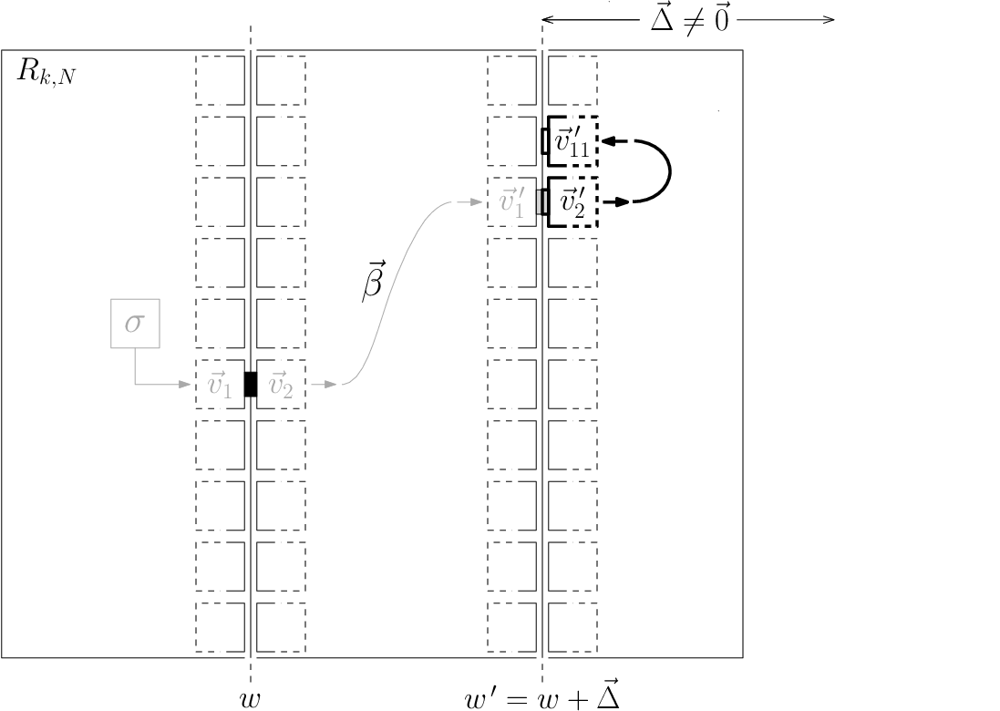
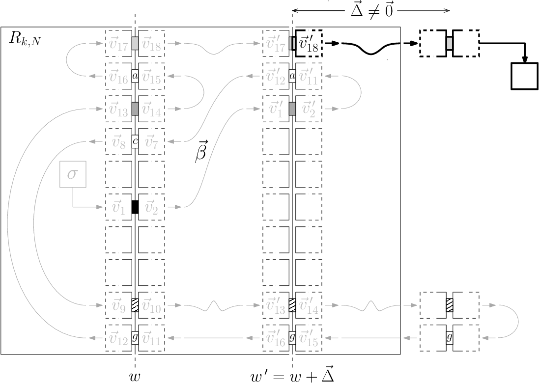
(a) The hypothesis. Note that α→\vec{\alpha} follows a simple path ss from the location of σ\sigma to a location in the furthest extreme column. The restricted glue window movies are sufficiently similar because their glues are at the same locations (up to translation), oriented in the same direction (away or toward σ\sigma), and each pair of glues that are placed by α→\vec{\alpha} at an “away crossing” of one of the windows is equal to its translated counterpart in the other window, e.g., the two topmost glues that touch ww and w′w^{\prime} are both light gray. The same constraint holds for all glue pairs shown with a solid shade of gray or a striped pattern. On the other hand, the glues adjacent to w′w^{\prime} that are placed by α→\vec{\alpha} at a “toward crossing”, for example g11′g^{\prime}_{11} and g12′g^{\prime}_{12}, are decorated with a letter in order to represent the fact that we do not assume that these glues are equal to their translated counterparts that touch ww (i.e., g15g_{15} and g16g_{16}).
Refer to caption
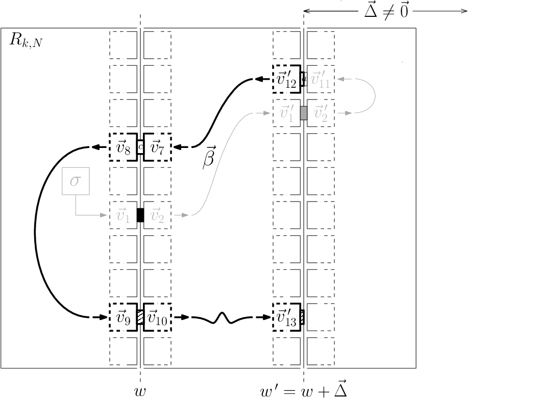
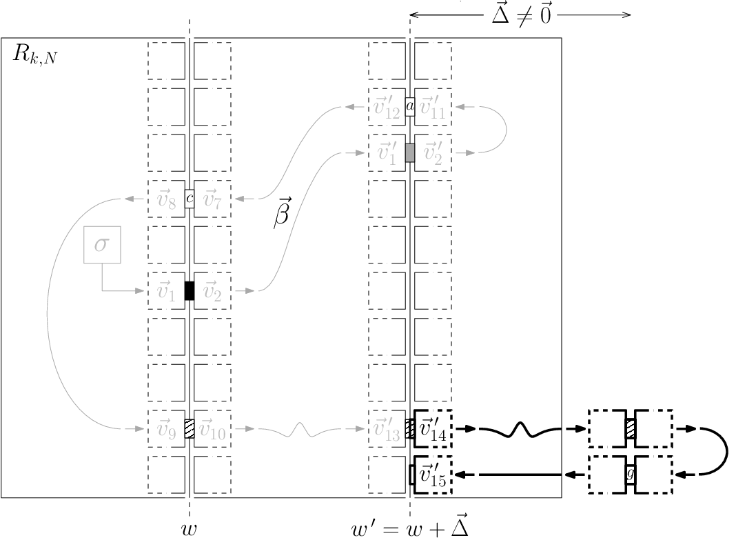
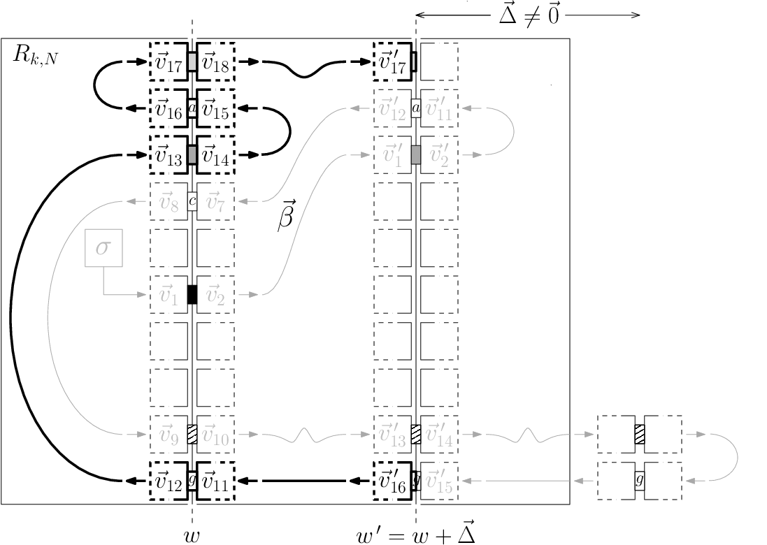
(b) The conclusion. Given the fact that 𝒯\mathcal{T} is directed and the way β→\vec{\beta} is defined, every pair of glues that touch ww must be equal to the corresponding pair of glues that touch w′w^{\prime} (if any). Thus, e.g., the glue pairs labelled bb and hh in part (2(a)) must really be equal to the glue pairs aa and gg, respectively. After β→\vec{\beta} places a tile at location v→17′\vec{v}^{\,\prime}_{17}, it will mimic how α→\vec{\alpha} got from v→18\vec{v}_{18} to the tile in the extreme column of Rk,NR_{k,N}, as depicted in part (2(a)). Since Δ→≠0→\vec{\Delta}\neq\vec{0}, this always results in at least one tile placement outside of Rk,NR_{k,N}. In this example, β\beta also happens to exit Rk,NR_{k,N} earlier in its assembly sequence, i.e., in the sub-path from v→14′\vec{v}^{\,\prime}_{14} to v→15′\vec{v}^{\,\prime}_{15}.
Figure 2: A 2D example of the hypothesis and conclusion of Lemma 2 for k=10k=10 and e=9e=9. Since the example is 2D, we use Rk,N={0,…,N−1}×{0,…,k−1}R_{k,N}=\{0,\ldots,N-1\}\times\{0,\ldots,k-1\}, rather than Rk,N3R^{3}_{k,N}.

We now give some notation that will be useful for our discussion of the proof of Lemma 2. The definitions and notation in the following paragraph are inspired by notation that first appeared in [7].

For a 𝒯\mathcal{T}-assembly sequence α→=(αi∣0≤i<l)\vec{\alpha}=(\alpha_{i}\mid 0\leq i<l), we write |α→|=l\left|\vec{\alpha}\right|=l. We write α→​[i]\vec{\alpha}[i] to denote x→↦t\vec{x}\mapsto t, where x→\vec{x} and tt are such that αi+1=αi+(x→↦t)\alpha_{i+1}=\alpha_{i}+\left(\vec{x}\mapsto t\right). We write α→​[i]+Δ→\vec{\alpha}[i]+\vec{\Delta}, for some vector Δ→\vec{\Delta}, to denote (x→+Δ→)↦t\left(\vec{x}+\vec{\Delta}\right)\mapsto t. If αi+1=αi+(x→↦t)\alpha_{i+1}=\alpha_{i}+\left(\vec{x}\mapsto t\right), then we write P​o​s​(α→​[i])=x→Pos\left(\vec{\alpha}[i]\right)=\vec{x} and T​i​l​e​(α→​[i])=tTile\left(\vec{\alpha}[i]\right)=t. Assuming |α→|>0\left|\vec{\alpha}\right|>0, the notation α→=α→+(x→↦t)\vec{\alpha}=\vec{\alpha}+\left(\vec{x}\mapsto t\right) denotes a tile placement step, namely the sequence of configurations (αi∣0≤i<l+1)\left(\alpha_{i}\mid 0\leq i<l+1\right), where αl\alpha_{l} is the configuration satisfying, αl​(x→)=t\alpha_{l}\left(\vec{x}\right)=t and for all y→≠x→\vec{y}\neq\vec{x}, αl​(y→)=αl−1​(y→)\alpha_{l}\left(\vec{y}\right)=\alpha_{l-1}\left(\vec{y}\right). Note that the “++” in a tile placement step is different from the “++” used in the notation “β=α+(p→↦t)\beta=\alpha+\left(\vec{p}\mapsto t\right)”. However, since the former operates on an assembly sequence, it should be clear from the context which operator is being invoked. The definition of a tile placement step does not require that the sequence of configurations be a 𝒯\mathcal{T}-assembly sequence. After all, the tile placement step α→=α→+(x→↦t)\vec{\alpha}=\vec{\alpha}+\left(\vec{x}\mapsto t\right) could be attempting to place a tile at a location that is not even adjacent to (a location in the domain of) αl−1\alpha_{l-1}. Or, it could be attempting to place a tile at a location that is in the domain of αl−1\alpha_{l-1}, which means a tile has already been placed at x→\vec{x}. So we say that such a tile placement step is correct if (αi∣0≤i<l+1)\left(\alpha_{i}\mid 0\leq i<l+1\right) is a 𝒯\mathcal{T}-assembly sequence. If |α→|=0\left|\vec{\alpha}\right|=0, then α→=α→+(x→↦t)\vec{\alpha}=\vec{\alpha}+\left(\vec{x}\mapsto t\right) results in the 𝒯\mathcal{T}-assembly sequence (α0)(\alpha_{0}), where α0\alpha_{0} is the assembly such that α0​(x→)=t\alpha_{0}\left(\vec{x}\right)=t and α0​(y→)\alpha_{0}\left(\vec{y}\right) is undefined at all other locations y→≠x→\vec{y}\neq\vec{x}.

In Figure 3, we define an algorithm that uses α→\vec{\alpha} to construct a new assembly sequence β→\vec{\beta} such that the tile placement steps by β→\vec{\beta} on the far side of w′w^{\prime} from the seed mimic a (possibly strict) subset of the tile placements by α→\vec{\alpha} on the far side of ww from the seed. When β→\vec{\beta} is on the near side of w′w^{\prime} to the seed, it mimics α→\vec{\alpha}, although β→\vec{\beta} does not necessarily mimic every tile placement by α→\vec{\alpha} on the near side of w′w^{\prime} to the seed. When β→\vec{\beta} crosses w′w^{\prime}, going away from the seed, by placing tiles at v→4​j−3′\vec{v}^{\prime}_{4j-3} and v→4​j−2′\vec{v}^{\prime}_{4j-2} in this order, then the tile it places at v→4​j−2′\vec{v}^{\prime}_{4j-2} is of the same type as the tile that α→\vec{\alpha} places at v→4​i−2=v→4​j−2′−Δ→\vec{v}_{4i-2}=\vec{v}^{\prime}_{4j-2}-\vec{\Delta}. After β→\vec{\beta} crosses w′w^{\prime} by placing a tile at v→4​j−2′\vec{v}^{\prime}_{4j-2}, β→\vec{\beta} places tiles that α→\vec{\alpha} places along ss from v→4​i−2\vec{v}_{4i-2} to v→4​i−1\vec{v}_{4i-1}, but the tiles β→\vec{\beta} places are translated to the far side of w′w^{\prime} from the seed. When β→\vec{\beta} is about to cross w′w^{\prime}, going toward the seed, by placing a tile at v→4​j−1′\vec{v}^{\prime}_{4j-1}, then, since 𝒯\mathcal{T} is directed, the type of tile that it places at this location is equal to the type of tile that α→\vec{\alpha} places at v→4​j−1′\vec{v}^{\prime}_{4j-1}. This means that β→\vec{\beta} may continue to follow ss but starting from v→4​j′\vec{v}^{\prime}_{4j}. Eventually, β→\vec{\beta} will finish crossing w′w^{\prime} going away from the seed for the last time by placing a tile at v→2​e+Δ→\vec{v}_{2e}+\vec{\Delta}. Then, β→\vec{\beta} places tiles that α→\vec{\alpha} places along ss, starting from v→2​e\vec{v}_{2e}, but the tiles that β→\vec{\beta} places are translated to the far side of w′w^{\prime} from the seed. Since Δ→≠0→\vec{\Delta}\neq\vec{0}, β→\vec{\beta} will ultimately place a tile that is not in Rk,N3R^{3}_{k,N}.

Figure 3: The algorithm for β→\vec{\beta}. Here, the variable “kk” has no relation to the “kk” used in Rk,N3R^{3}_{k,N}.


Initialize j=1j=1, k=0k=0 and β→=()\vec{\beta}=\left(\right) 1
while P​o​s​(α→​[k])≠v→4​j−2′Pos\left(\vec{\alpha}[k]\right)\neq\vec{v}^{\prime}_{4j-2} do /* Loop 1 */ 2
β→=β→+α→​[k]\vec{\beta}=\vec{\beta}+\vec{\alpha}[k] 3
   k=k+1k=k+1 4
while v→4​j−2′≠v→2​e+Δ→\vec{v}^{\prime}_{4j-2}\neq\vec{v}_{2e}+\vec{\Delta} do /* Loop 2 */ 5
6
   Let ii be such that 4​i−24i-2 is the index of v→4​j−2′−Δ→\vec{v}^{\prime}_{4j-2}-\vec{\Delta} in MM 7
   Let kk be such that P​o​s​(α→​[k])=v→4​i−2Pos\left(\vec{\alpha}[k]\right)=\vec{v}_{4i-2} 8
   while P​o​s​(α→​[k])≠v→4​iPos\left(\vec{\alpha}[k]\right)\neq\vec{v}_{4i} do /* Loop 2a */ 9
    β→=β→+(α→​[k]+Δ→)\vec{\beta}=\vec{\beta}+\left(\vec{\alpha}[k]+\vec{\Delta}\right) 10
      k=k+1k=k+1 11
   Let j′j^{\prime} be such that 4​j′4j^{\prime} is the index of v→4​i+Δ→\vec{v}_{4i}+\vec{\Delta} in M′M^{\prime} 12
   Let kk be such that P​o​s​(α→​[k])=v→4​j′′Pos\left(\vec{\alpha}[k]\right)=\vec{v}^{\prime}_{4j^{\prime}} 13
   while P​o​s​(α→​[k])≠v→4​j′+2′Pos\left(\vec{\alpha}[k]\right)\neq\vec{v}^{\prime}_{4j^{\prime}+2} do /* Loop 2b */ 14
    β→=β→+α→​[k]\vec{\beta}=\vec{\beta}+\vec{\alpha}[k] 15
      k=k+1k=k+1 16
   j=j′+1j=j^{\prime}+1 17
   Let kk be such that P​o​s​(α→​[k])=v→2​ePos\left(\vec{\alpha}[k]\right)=\vec{v}_{2e} 18
while k<|α→|k<\left|\vec{\alpha}\right| do /* Loop 3 */ 19
β→=β→+(α→​[k]+Δ→)\vec{\beta}=\vec{\beta}+\left(\vec{\alpha}[k]+\vec{\Delta}\right) 20
   k=k+1k=k+1 21
return β→\vec{\beta} 22

We illustrate the behavior of this algorithm in Figure 4, where we apply it to the assembly sequence α→\vec{\alpha} shown in Figure 2(a).

We must show that all of the tile placement steps executed by the algorithm for β→\vec{\beta} are correct. In addition, we must also prove that the tile placement steps executed by the algorithm for β→\vec{\beta} place tiles along a simple path. Let α→=α→+(x→′↦t′)\vec{\alpha}=\vec{\alpha}+\left(\vec{x}^{\prime}\mapsto t^{\prime}\right) and α→=α→+(x→↦t)\vec{\alpha}=\vec{\alpha}+\left(\vec{x}\mapsto t\right) be consecutive tile placement steps executed by the algorithm for β→\vec{\beta} and assume that the former is either the first tile placement step executed or it is correct. To show that the latter is correct, we will show that:

  1. a

    the tile configuration that consists of tt placed at x→\vec{x} and t′t^{\prime} placed at x→′\vec{x}^{\prime} is a 11-stable assembly (not necessarily 𝒯\mathcal{T}-producible) whose domain consists of two locations, and

  2. b

    the location x→\vec{x} is unoccupied before α→=α→+(x→↦t)\vec{\alpha}=\vec{\alpha}+\left(\vec{x}\mapsto t\right) is executed.

The previous two conditions constitute a slightly stronger notion of “correctness” for a tile placement step, which we will call adjacently correct. After all, the two previous conditions imply that α→=α→+(x→↦t)\vec{\alpha}=\vec{\alpha}+\left(\vec{x}\mapsto t\right) is correct, but if α→=α→+(x→↦t)\vec{\alpha}=\vec{\alpha}+\left(\vec{x}\mapsto t\right) is correct, then condition b must hold but condition a need not because x→\vec{x} does not have to be adjacent to x→′\vec{x}^{\prime}. It suffices to prove that every tile placement step executed by the algorithm for β→\vec{\beta} is adjacently correct. As a result, β→\vec{\beta}, like α→\vec{\alpha}, will place tiles along a simple path.
Refer to caption
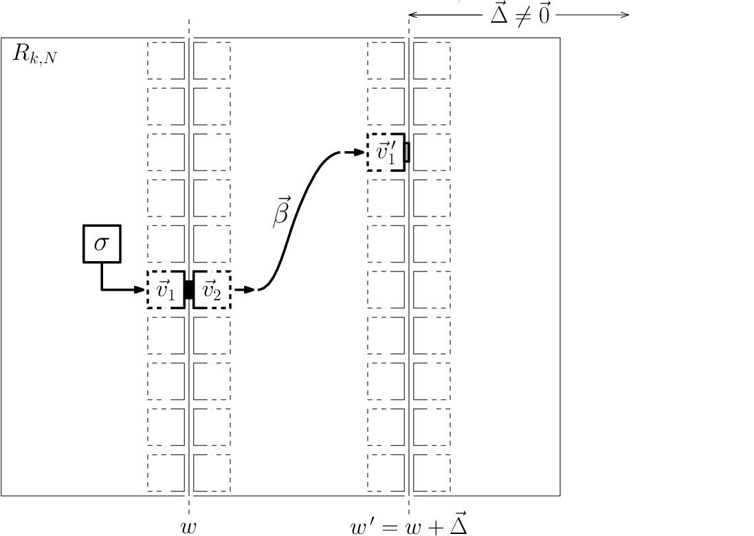
(a) Right after Loop 1 has completed: The α→\vec{\alpha} sub-path from σ\sigma to v→1′\vec{v}^{\,\prime}_{1} was used to initialize β→\vec{\beta}.
Refer to caption
(b) Right after Loop 2a has completed for the first time: The α→\vec{\alpha} sub-path from v→14\vec{v}_{14} to v→15\vec{v}_{15} was translated by Δ→\vec{\Delta} and appended to β→\vec{\beta}.
Refer to caption
(c) Right after Loop 2b has completed for the first time: The α→\vec{\alpha} sub-path from v→12′\vec{v}^{\,\prime}_{12} to v→13′\vec{v}^{\,\prime}_{13} was appended to β→\vec{\beta}.
Refer to caption
(d) Right after Loop 2a has completed for the second time: The α→\vec{\alpha} sub-path from v→10\vec{v}_{10} to v→11\vec{v}_{11} was translated by Δ→\vec{\Delta} and appended to β→\vec{\beta}.
Refer to caption
(e) Right after Loop 2b has completed for the second time: The α→\vec{\alpha} sub-path from v→16′\vec{v}^{\,\prime}_{16} to v→17′\vec{v}^{\,\prime}_{17} was appended to β→\vec{\beta}.
Refer to caption
(f) Right after Loop 3 (and the algorithm) has completed: The α→\vec{\alpha} suffix starting with v→18\vec{v}_{18} was translated by Δ→\vec{\Delta} and appended to β→\vec{\beta}.
Figure 4: The trace of the algorithm shown in Figure 3 when applied to the assembly sequence α→\vec{\alpha} shown in Figure 2(a). In each sub-figure, the new sub-path is bolded and is a continuation of the sub-path in the previous one. The last sub-figure above shows the same assembly sequence β→\vec{\beta} depicted in Figure 2(b).

See Section A for the full proof of Lemma 2. We now have the necessary machinery for our lower bound, which is the following.

Theorem 1.

KU​S​A1​(Rk,N3)=Ω⁡(N1k)K^{1}_{USA}\left(R^{3}_{k,N}\right)=\Omega\left(N^{\frac{1}{k}}\right).

The proof idea for Theorem 1 is as follows. Assume 𝒯=(T,σ,1)\mathcal{T}=(T,\sigma,1) is a directed, 3D TAS in which Rk,N3R^{3}_{k,N} self-assembles. By Lemmas 1 and 2, N≤3⋅|G|k⋅k⋅16kN\leq 3\cdot|G|^{k}\cdot k\cdot 16^{k}, where GG is the set of all glues in TT. This means that |T|≥N1k576=Ω⁡(N1k)|T|\geq\frac{N^{\frac{1}{k}}}{576}=\Omega\left(N^{\frac{1}{k}}\right). See Section A for the full proof of Theorem 1.

Theorem 1 says that temperature-1 self-assembly in just-barely 3D is no more powerful than temperature-2 self-assembly in 2D. Interestingly, our lower bound for KU​S​A1​(Rk,N3)K^{1}_{USA}\left(R^{3}_{k,N}\right) matches the lower bound for KS​A1​(Rk,N3)K^{1}_{SA}\left(R^{3}_{k,N}\right) by Furcy, Summers and Wendlandt [6] but our bound is much more interesting than theirs because ours is roughly the square root of the best known upper bound, to which we turn our attention.

4 The upper bound

In this section, we give a construction that outputs aTAS in which a sufficiently large rectangle (of any height k≥2k\geq 2) Rk,N3R^{3}_{k,N} uniquely self-assembles, testifying to our upper bound, which is roughly the square of our lower bound.

Theorem 2.

KU​S​A1​(Rk,N3)=O⁡(N1⌊k2⌋+log⁡N)K^{1}_{USA}\left(R^{3}_{k,N}\right)=O\left(N^{\frac{1}{\left\lfloor\frac{k}{2}\right\rfloor}}+\log N\right).

Assume that k>3k>3, otherwise the construction is trivial. We use a counter whose base depends on the dimensions of the target rectangle. Let w=⌊k2⌋w=\left\lfloor\frac{k}{2}\right\rfloor be the width (number of digits) of the counter. The base of the counter is M=⌈(N31)1w⌉M=\left\lceil\left(\frac{N}{31}\right)^{\frac{1}{w}}\right\rceil. The value of each digit is represented in binary, using a series of m=⌈log⁡M⌉m=\left\lceil\log M\right\rceil bit bumps that protrude from a horizontal line of tiles. Each bit bump geometrically encodes one bit as a corresponding assembly of tiles.

A novel and noteworthy feature of our construction is the organization of the digits of the counter into pairs of digits, where each pair of digits is contained within a rectangular digit region. We say that a digit region is a general digit region if its dimensions are four rows by l=9​m+22l=9m+22 columns. If kmod4=0k\mod 4=0, then each general digit region, of which there are w2\frac{w}{2}, contains two digits. We will use a special digit region with two rows and ll columns to handle the case where kmod4=2k\mod 4=2. Going forward, we will refer to a general digit region as simply a digit region. Throughout this section, we will assume kmod4=0k\mod 4=0.

Refer to caption
Figure 5: This example shows how the digits that comprise a value of the counter are organized into digit regions. The next value of the counter would have a similar organization, to the east of the current value (see Figure 7). In this example, since k=12k=12, the value of the counter has six digits, d0d_{0} through d5d_{5}, the latter being the most significant digit and the former the least significant. Even (odd) digits have even (odd) subscripts. In this example, each digit is encoded using two bits. The extra bit for odd digits indicates whether that digit is the most significant digit. Note that the least significant (westernmost) bit of d5d_{5} is darkened to indicate that its value is 1, because d5d_{5} is the most significant digit. Although this is a specific example, the general dimensions are given. Note that we include an “extra” Θ⁡(m)\Theta\left(m\right) columns in a general digit region in order to contain the most significant digit of the counter within a “special” digit region comprised of only two rows and ll columns, in the case where kmod4=2k\mod 4=2.

The westernmost digit within a general digit region is even, and its bit bumps face toward the south. The easternmost digit is odd, and its bit bumps face toward the north. The westernmost bit of each odd digit encodes whether that digit is the most significant digit that is contained in a general digit region. Figure 5 shows a high-level overview of how the digits (that comprise a value) of the counter are organized into digit regions.

A gadget, referred to by a name like Gadget, is a group of tiles that perform a specific task as they self-assemble. Each gadget, except for the seed-containing gadget, has one input glue and at least one output glue. For each gadget, the placement of the input and output glues can be inferred from the way the new gadgets bind to the assembly shown in the preceding figure. Glues internal to the gadget are configured to ensure unique self-assembly within the gadget. The strength of every glue is 1. If a glue contains some information xx, this means that the glue label has a structure that contains the encoding of xx, according to some fixed, standard encoding scheme.

We initialize the counter to start at a certain initial value ss, padded out to ww digits, with leading 0s. In order to choose the initial value, let n=⌊Nl⌋−1n=\left\lfloor\frac{N}{l}\right\rfloor-1 be the number of increment steps. Then, we set s=Mw−ns=M^{w}-n to be the initial value. Then, once ss is set, a tile assembly representation of ss self-assembles via a series of gadgets. Figure 6 shows a fully assembled example for s=333332s=333332.

Refer to caption
Figure 6: A fully assembled example of the initial value of the counter for s=333332s=333332. Following standard presentation conventions for just-barely 3D tile self-assembly, we use big squares to represent tiles placed in the z=0z=0 plane and small squares to represent tiles placed in the z=1z=1 plane. A glue between a z=0z=0 tile and z=1z=1 tile is denoted as a small disk. Glues between z=0z=0 tiles are denoted as thick lines. Glues between z=1z=1 tiles are denoted as thin lines. The leftmost tile in the z=0z=0 plane is the seed tile.

After the initial value of the counter self-assembles (see Figures 35 through 44 in Section B.1), the counter undergoes a series of increment operations. Each increment operation increments the value of the counter by one. The counter counts up to the highest possible value, as determined by its base and the number of digits, increments once more to roll over to 0, and then stops. Finally, one could use O⁡(Nmodl)=O⁡(l)O(N\mod l)=O(l) filler tiles to fill in the remaining columns of the rectangle (we actually never explicitly specify this trivial step in our construction). Figure 7 shows a high-level, artificial example of the behavior of the counter in terms of its increment steps.

Refer to caption
Figure 7: In this artificial example, M=4M=4 and s=333332s=333332. The counter increments through 333333333333 and rolls over to 000000000000 before stopping. Each digit region is outlined. For each digit region (other than a digit region that contains a digit of the final value of the counter), the digit region to its east is the corresponding digit region.

The basic idea of the general self-assembly algorithm for incrementing the value of the counter is to read an even digit in the current digit region, write its result in the corresponding digit region, come back to the current digit region and read the odd digit, write its result in the corresponding digit region. Then, do the same thing in the digit region in which the next two most significant digits are contained and stop after the most significant digit was read and the result was written.

The trick is to read each digit from the current digit region and write the respective result in the corresponding digit region without having to hard-code into the glues of the tiles both Θ⁡(m)\Theta\left(m\right) bits (representing the binary representation of the value of the digit that was just read), as well as the relative location along a path whose length is Θ⁡(l)\Theta(l). To accomplish this, we use gadgets whose names are prefixed with Repeating_after_ and Stopper_after_.

In Figures 8 through 33, we create the gadgets that implement the general self-assembly algorithm that increments the value of the counter. Figures 8 through 33 also show an example assembly sequence, where, unless specified otherwise, each figure continues the sequence from the resulting assembly in the previously-numbered figure, unless explicitly stated otherwise.

Refer to caption
Figure 8: A Read_non_MSB gadget is shown here. A Read_non_MSB gadget reads the value of a bit that is not the most significant bit of a digit. The depicted gadget is a Read_non_MSB_0 gadget. For every digit region except the southernmost one, the Start_digit_region gadget in Figure 33 exposes output glues in both the z=0z=0 and z=1z=1 planes, from which only the correct Read_non_MSB gadget self-assembles. Otherwise, for the southernmost digit region, a Reset_read_even_digit gadget is used (see Figure 30). The last tile in a Read_non_MSB gadget guesses the value of the next bit. The input glue of a Read_non_MSB gadget being created here contains a binary string x∈{0,1}ix\in\{0,1\}^{i}, for 1≤i<m1\leq i<m, where the rightmost bit is the bit that this gadget reads. The two output glues contain xx followed by the value of the next bit that will be read, i.e., x​0x0 and x​1x1. The input glues of the Read_non_MSB gadgets being created here also contain a bit set to 0, which is the parity of the digit (even or odd) whose bits are being read, which, in this case, is even. This will allow us to use the general Read_non_MSB gadgets to create specific gadgets to read the bits of both even and odd digits, respectively. In general, we create O⁡(1)O(1) Read_non_MSB gadgets for each x∈{0,1}ix\in\{0,1\}^{i}, for 1≤i<m1\leq i<m, contributing O⁡(M)O(M) tile types.
Refer to caption
Figure 9: A Read_MSB gadget is shown here. A Read_MSB gadget reads the value of the most significant bit of a digit. The input glue of a Read_MSB gadget being created here contains a binary string x∈{0,1}mx\in\{0,1\}^{m} and its output glue will also contain xx. The rightmost bit of xx is the most significant bit of the digit that was just read. The input glues of the Read_MSB gadgets being created here also contain a bit set to 0, which is the parity of the digit (even or odd) whose bits were read, which, in this case, is even. This will allow us to use the general Read_MSB gadgets to create specific gadgets to read the MSBs of both even and odd digits, respectively. In general, we create O⁡(1)O(1) Read_MSB gadgets for each x∈{0,1}mx\in\{0,1\}^{m}, contributing O⁡(M)O(M) tile types.
Refer to caption
Figure 10: A path of Repeating_after_even_digit gadgets is shown here. The Repeating_after_even_digit gadget initiates the attachment of another Repeating_after_even_digit tile, continuing the self-assembly of a path of repeating tiles toward and ultimately blocked from continuing by a Stopper_after_odd_digit gadget. We use Repeating_after_even_digit (and Repeating_after_odd_digit) gadgets to propagate Θ⁡(m)\Theta(m) bits along an arbitrarily long path of tiles, without also having the glues of the tiles along the path contain the relative location of each tile within the path. All gadgets whose name starts with Repeating_after essentially “forget” where they are and self-assemble in a line, until they cannot. In general, we create O⁡(1)O(1) Repeating_after_even_digit gadgets for each x∈{0,1}mx\in\{0,1\}^{m}, contributing O⁡(M)O(M) tile types.
Refer to caption
Refer to caption
Figure 11: An At_stopper_after_odd_digit gadget is shown here. It has a fixed size. The At_stopper_after_odd_digit gadget spans two adjacent digit regions. The black portion is in the current digit region and the gray portion is in the corresponding digit region. In general, if a gadget spans the current and corresponding digit regions, then the portion in the latter is depicted in gray and the former in black. The self-assembly of an At_stopper_after_odd_digit gadget is initiated by the north-facing glue of the last Repeating_after_even_digit gadget to attach in the path in Figure 10. If x∈{0,1}mx\in\{0,1\}^{m} and c∈{0,1}c\in\{0,1\} are contained in the output glue of the latter, where c=1c=1 indicates the presence of an arithmetic carry and c=0c=0 otherwise, then the output glue of the former contains the mm-bit binary representation of (x+c)modM\left(x+c\right)\mod M. If (x+c)modM=0\left(x+c\right)\mod M=0, then c=1c=1 is contained in the output glue of the gadgets being created here. In general, we create O⁡(1)O(1) At_stopper_after_odd_digit gadgets for each x∈{0,1}mx\in\{0,1\}^{m}, contributing O⁡(M)O(M) tile types.
Refer to caption
Figure 12: A series of two Write_even_digit gadgets is shown here. Intuitively, Write gadgets “undo” what the Read gadgets do. To that end, the input glue of a Write_even_digit gadget being created here contains a binary string b​xbx, where b∈{0,1}b\in\{0,1\}, and x∈{0,1}ix\in\{0,1\}^{i}, for 0≤i<m0\leq i<m, its output glue contains xx, and the corresponding bit bump for bb self-assembles. In general, we create O⁡(1)O(1) Write_even_digit gadgets for each x∈{0,1}ix\in\{0,1\}^{i}, for 0≤i<m0\leq i<m, contributing O⁡(M)O(M) tile types.
Refer to caption
Figure 13: A Stopper_after_even_digit gadget is shown here. A Stopper_after_even_digit gadget is used to stop a subsequent path of Repeating_after_odd_digit gadgets that will be propagating the value of an odd digit as they self-assemble. In general, we create O⁡(1)O(1) Stopper_after_even_digit gadgets, contributing O⁡(1)O(1) tile types.
Refer to caption
Figure 14: A path of Single_tile_opposite gadgets is shown here. We create O⁡(1)O(1) Single_tile_opposite gadgets for each location in the general version of the depicted path of length 3​m+43m+4, contributing O⁡(m)O(m) tile types.
Refer to caption
Refer to caption
Figure 15: A Between_digit_regions gadget, originating in the corresponding digit region (bottom) and terminating back in the current digit region (top), is shown here. In general, we create O⁡(1)O(1) Between_digit_regions, contributing O⁡(1)O(1) tile types.
Refer to caption
Figure 16: A path of Single_tile_opposite gadgets is shown here. We create O⁡(1)O(1) Single_tile_opposite gadgets for each location in the general version of the depicted path of length 3​m+73m+7, contributing O⁡(m)O(m) tile types.
Refer to caption
Figure 17: An At_MSB_of_odd_digit gadget is shown here. In general, we create O⁡(1)O(1) At_MSB_of_odd_digit gadgets, contributing O⁡(1)O(1) tile types.
Refer to caption
Figure 18: A path of Single_tile_opposite gadgets is shown here. We create O⁡(1)O(1) Single_tile_opposite gadgets for each location in the general version of the depicted path of length 3​(m+1)3\left(m+1\right), contributing O⁡(m)O(m) tile types.
Refer to caption
Figure 19: A Start_read_odd_digit gadget is shown here. A Start_read_odd_digit, like a Start_digit_region gadget from Figure 33 does for an even digit, “guesses” the value of the most significant digit indicator bit in an odd digit by exposing output glues in both the z=0z=0 and z=1z=1 planes. In general, we create O⁡(1)O(1) Start_read_odd_digit gadgets, contributing O⁡(1)O(1) tile types. The Read_ gadgets for the odd digit that attach to this gadget (and are depicted in Figure 20) are created in a similar manner and contribute the same number of tile types as the Read_ gadgets for the even digits (see Figures 8 and 9), except the input glues of the former gadgets contain a bit set to 1, which is the parity of the digit whose bits were being read.
Refer to caption
Refer to caption
Figure 20: A path of Repeating_after_odd_digit gadgets is shown here. This path is eventually hindered by a Stopper_after_even_digit gadget (see Figure 13). In general, we create O⁡(1)O(1) Repeating_after_odd_digit gadgets for each x∈{0,1}m+1x\in\{0,1\}^{m+1}, contributing O⁡(M)O(M) tile types.
Refer to caption
Figure 21: An At_stopper_after_even_digit gadget is shown here. It has a fixed size. The south-facing glue of the last Repeating_after_odd_digit gadget to attach in the path shown in Figure 20 will initiate the self-assembly of an At_stopper_after_even_digit gadget. If, for b∈{0,1}b\in\{0,1\} and x∈{0,1}mx\in\{0,1\}^{m}, b​xbx and c∈{0,1}c\in\{0,1\} are contained in the output glue of the former, where c=1c=1 indicates the presence of an arithmetic carry and c=0c=0 otherwise, then the output glue of the latter contains the result of prepending bb to the mm-bit binary representation of (x+c)modM\left(x+c\right)\mod M. If (x+c)modM=0\left(x+c\right)\mod M=0, then c=1c=1 is contained in the output glue of the gadgets being created here. In general, we create O⁡(1)O(1) At_stopper_after_even_digit gadgets for each b​x∈{0,1}m+1bx\in\{0,1\}^{m+1}, contributing O⁡(M)O(M) tile types.
Refer to caption
Figure 22: A series of three Write_odd_digit gadgets is shown here. The input glue of a Write_odd_digit gadget being created here contains a binary string b​xbx, where b∈{0,1}b\in\{0,1\}, and x∈{0,1}ix\in\{0,1\}^{i}, for 0≤i≤m0\leq i\leq m, its output glue contains xx, and the corresponding bit bump for bb will self-assemble. In general, we create O⁡(1)O(1) Write_odd_digit gadgets for each x∈{0,1}ix\in\{0,1\}^{i}, for 0≤i≤m0\leq i\leq m, contributing O⁡(M)O(M) tile types.
Refer to caption
Figure 23: A path of Single_tile gadgets is shown here. We create O⁡(1)O(1) Single_tile gadgets for each location in the general version of the depicted path of length 3​m+33m+3, contributing O⁡(m)O(m) tile types.
Refer to caption
Figure 24: A Stopper_after_odd_digit gadget is shown here. The Stopper_after_odd_digit gadget geometrically marks the location of (a constant distance from) the easternmost edge of the current digit region in which it self-assembles. It will ultimately block a subsequent path of repeating tiles that will be propagating the value of an even digit from the current digit region to the corresponding adjacent digit region for the next value of the counter. In general, we create O⁡(1)O(1) Stopper_after_odd_digit gadgets, contributing O⁡(1)O(1) tile types.
Refer to caption
Figure 25: A path of Single_tile_opposite gadgets is shown here. We create O⁡(1)O(1) Single_tile_opposite gadgets for each location in the general version of the depicted path of length 1+3​(m+1)+(8+3​m−4)+11+3\left(m+1\right)+\left(8+3m-4\right)+1, contributing O⁡(m)O(m) tile types.
Refer to caption
Figure 26: A Between_digits gadget is shown here. In general, we create O⁡(1)O(1) Between_digits gadgets, contributing O⁡(1)O(1) tile types.
Refer to caption
Figure 27: A path of Single_tile_opposite gadgets is shown here. If the odd digit that just self-assembled is the most significant digit and the value of the counter did not roll over to 0, then turn the corner (see the Reset_turn_corner gadget in Figure 28) and return to execute another increment operation. If the value of the counter rolled over to 0, which could have been detected by the last Write_odd_digit gadget created in Figure 22, then no further increment operations are executed. We create O⁡(1)O(1) Single_tile_opposite gadgets for each location in the general version of the depicted path of length 3​m+63m+6, contributing O⁡(m)O(m) tile types.
Refer to caption
Figure 28: A Reset_turn_corner gadget is shown here. In general, we create one Reset_turn_corner gadget, contributing O⁡(1)O(1) tile types.
Refer to caption
Figure 29: A (beginning portion of a) path of Reset_single_tile gadgets is shown here. Note that a Reset_single_tile gadget is comprised of a single tile whose input glue is always north-facing, and whose output glue is always south-facing. We create one Reset_single_tile gadget for each location in the general version of the depicted path of length k−2k-2, contributing O⁡(k)O(k) tile types.
Refer to caption
Figure 30: The Reset_read_even_digit gadget is shown here. The Reset_read_even_digit gadget initiates the execution of the next increment step. The Reset_read_even_digit gadget “guesses” the value of the first bit in the least significant digit by exposing output glues in both the z=0z=0 and z=1z=1 planes. In general, we create one Reset_read_even_digit gadget, contributing O⁡(1)O(1) tile types.
Refer to caption
Figure 31: A Z1_to_z0 gadget is shown here. If the odd digit that just self-assembled is not the most significant digit, then proceed back to the current digit region and ultimately into the digit region in which the next two most significant digits are contained. This gadget transitions the path of Single_tile_opposite gadgets from Figure 27 from the z=1z=1 plane to the z=0z=0 plane in order to ensure a clear path in the z=1z=1 plane for a subsequent path of Reset_single_tile gadgets (see Figure 29). In general, we create O⁡(1)O(1) Z1_to_z0 gadgets, contributing O⁡(1)O(1) tile types.
Refer to caption
Refer to caption
Figure 32: A path of Single_tile_opposite gadgets is shown here. A Start_digit_region gadget (created in Figure 33) binds to the west-facing glue of the last Single_tile_opposite in the depicted path. We create O⁡(1)O(1) Single_tile_opposite gadgets for each location in the general version of the depicted path of length 3​m+6+3​(m+1)+8+3​m+1+13m+6+3\left(m+1\right)+8+3m+1+1, contributing O⁡(m)O(m) tile types.
Refer to caption
Figure 33: A Start_digit_region gadget is shown here. A Start_digit_region gadget “guesses” the value of the least significant bit in a non-least significant even digit by exposing output glues in both the z=0z=0 and z=1z=1 planes. The value of the least significant bit in the least significant digit is guessed by the Reset_read_even_digit gadget created in Figure 30. In general, we create O⁡(1)O(1) Start_digit_region gadgets, contributing O⁡(1)O(1) tile types.

If NN is assumed to be sufficiently large, then the total number of tile types contributed by all the gadgets that were created in Figures 8 through 33 when kmod4=0k\mod 4=0, is O⁡(M+m+k)O(M+m+k). Moreover, the total number of tile types contributed by all the gadgets that we use to self-assemble the initial value is O⁡(k​m)O(km) (see Figures 35 through 44 in Section B.1). Note that k​m=k⁡⌈log⁡⌈(N31)1w⌉⌉=k⁡⌈log⁡(N31)1w⌉≤2​k​log​N1w=2​kw​log​N=2​k⌊k2⌋​log​N≤2​kk3​log​N=O⁡(log⁡N)km=k\left\lceil\log\left\lceil\left(\frac{N}{31}\right)^{\frac{1}{w}}\right\rceil\right\rceil=k\left\lceil\log\left(\frac{N}{31}\right)^{\frac{1}{w}}\right\rceil\leq 2k\log N^{\frac{1}{w}}=\frac{2k}{w}\log N=\frac{2k}{\left\lfloor\frac{k}{2}\right\rfloor}\log N\leq\frac{2k}{\frac{k}{3}}\log N=O(\log N) and M=⌈(N31)1w⌉=⌈(N31)1⌊k2⌋⌉=O⁡(N1⌊k2⌋)M=\left\lceil\left(\frac{N}{31}\right)^{\frac{1}{w}}\right\rceil=\left\lceil\left(\frac{N}{31}\right)^{\frac{1}{\left\lfloor\frac{k}{2}\right\rfloor}}\right\rceil=O\left(N^{\frac{1}{\left\lfloor\frac{k}{2}\right\rfloor}}\right). Thus, the size of the tile set output by our construction, when kmod4=0k\mod 4=0, is O⁡(N1⌊k2⌋+log⁡N)O\left(N^{\frac{1}{\left\lfloor\frac{k}{2}\right\rfloor}}+\log N\right). Observe that, if Rk,N3R^{3}_{k,N} is a thin rectangle, then k<log⁡Nlog⁡log⁡N−log⁡log⁡log⁡N<log⁡Nlog⁡log⁡N−13​log⁡log​N=32​log⁡Nlog⁡log⁡Nk<\frac{\log N}{\log\log N-\log\log\log N}<\frac{\log N}{\log\log N-\frac{1}{3}\log\log N}=\frac{\frac{3}{2}\log N}{\log\log N}, and we have log⁡N=2log⁡log⁡N=(N1log⁡N)log⁡log⁡N=N3232​log⁡Nlog⁡log⁡N=O⁡(N32k)=O⁡(N1k2)=O⁡(N1⌊k2⌋)\log N=2^{\log\log N}=\left(N^{\frac{1}{\log N}}\right)^{\log\log N}=N^{\frac{\frac{3}{2}}{\frac{\frac{3}{2}\log N}{\log\log N}}}=O\left(N^{\frac{\frac{3}{2}}{k}}\right)=O\left(N^{\frac{1}{\frac{k}{2}}}\right)\ =\ O\left(N^{\frac{1}{\left\lfloor\frac{k}{2}\right\rfloor}}\right).

The case of kmod4=2k\mod 4=2 can be handled similarly, using a special case digit region in which the most significant digit is represented using two rows and ll columns (see Section B.2).

The cases where kmod4∈{1,3}k\mod 4\in\{1,3\} can be handled by using O⁡(1)O(1) tiles that self-assemble into an additional row.

The full details for our construction, in which all cases are handled, can be found in Section B.3.

5 Future work

In this paper, we gave improved bounds on KU​S​A1​(Rk,N3)K^{1}_{USA}\left(R^{3}_{k,N}\right). Specifically, our upper bound, O⁡(N1⌊k2⌋+log⁡N)O\left(N^{\frac{1}{\left\lfloor\frac{k}{2}\right\rfloor}}+\log N\right), is roughly the square of our lower bound, Ω⁡(N1k)\Omega\left(N^{\frac{1}{k}}\right). However, questions still remain, upon which we feel future work should be based. Is it the case that either KS​A1​(Rk,N3)K^{1}_{SA}\left(R^{3}_{k,N}\right) or KU​S​A1​(Rk,N3)K^{1}_{USA}\left(R^{3}_{k,N}\right) is equal to O⁡(N1k+k)O\left(N^{\frac{1}{k}}+k\right)? If not, then what are tight bounds for KS​A1​(Rk,N3)K^{1}_{SA}\left(R^{3}_{k,N}\right) and KU​S​A1​(Rk,N3)K^{1}_{USA}\left(R^{3}_{k,N}\right)?

References

  • [1] Leonard M. Adleman, Qi Cheng, Ashish Goel, and Ming-Deh A. Huang, Running time and program size for self-assembled squares, Proceedings of the Thirty-Third Annual ACM Symposium on Theory of Computing (STOC), 2001, pp. 740–748.
  • [2] Gagan Aggarwal, Qi Cheng, Michael H. Goldwasser, Ming-Yang Kao, Pablo Moisset de Espanés, and Robert T. Schweller, Complexities for generalized models of self-assembly, SIAM Journal on Computing (SICOMP) 34 (2005), 1493–1515.
  • [3] Matthew Cook, Yunhui Fu, and Robert T. Schweller, Temperature 1 self-assembly: Deterministic assembly in 3D and probabilistic assembly in 2D, Proceedings of the Twenty-Second Annual ACM-SIAM Symposium on Discrete Algorithms (SODA), 2011, pp. 570–589.
  • [4] David Furcy, Samuel Micka, and Scott M. Summers, Optimal program-size complexity for self-assembled squares at temperature 1 in 3D, Algorithmica 77 (2017), no. 4, 1240–1282.
  • [5] David Furcy and Scott M. Summers, Optimal self-assembly of finite shapes at temperature 1 in 3D, Algorithmica 80 (2018), no. 6, 1909–1963.
  • [6] David Furcy, Scott M. Summers, and Christian Wendlandt, New bounds on the tile complexity of thin rectangles at temperature-1, Proceedings of the Twenty-Fifth International Conference on DNA Computing and Molecular Programming, (DNA 25), vol. 11648, 2019, pp. 100–119.
  • [7] P.-E. Meunier, M. J. Patitz, S. M. Summers, G. Theyssier, A. Winslow, and D. Woods, Intrinsic universality in tile self-assembly requires cooperation, Proceedings of the Twenty-Fifth Annual ACM-SIAM Symposium on Discrete Algorithms (SODA), 2014, pp. 752–771.
  • [8] Paul W. K. Rothemund and Erik Winfree, The program-size complexity of self-assembled squares (extended abstract), The Thirty-Second Annual ACM Symposium on Theory of Computing (STOC), 2000, pp. 459–468.
  • [9] Nadrian C. Seeman, Nucleic-acid junctions and lattices, Journal of Theoretical Biology 99 (1982), 237–247.
  • [10] David Soloveichik and Erik Winfree, Complexity of self-assembled shapes, SIAM Journal on Computing (SICOMP) 36 (2007), no. 6, 1544–1569.
  • [11] Hao Wang, Proving theorems by pattern recognition – II, The Bell System Technical Journal XL (1961), no. 1, 1–41.
  • [12] Erik Winfree, Algorithmic self-assembly of DNA, Ph.D. thesis, California Institute of Technology, June 1998.

Appendix A Lower bound appendix

This section contains all the proofs related to our lower bound.

Lemma 1.

Assume: 𝒯=(T,σ,1)\mathcal{T}=(T,\sigma,1) is a 3D TAS, GG is the set of all glues in TT, k,N∈ℤ+k,N\in\mathbb{Z}^{+}, ss is a simple path starting from the location of σ\sigma such that s⊆Rk,N3s\subseteq R^{3}_{k,N}, α→\vec{\alpha} is a sequence of 𝒯\mathcal{T}-producible assemblies that follows ss, m∈ℤ+m\in\mathbb{Z}^{+}, for all 1≤l≤m1\leq l\leq m, wlw_{l} is a window, for all 1≤l<l′≤m1\leq l<l^{\prime}\leq m, Δ→l,l′≠0→\vec{\Delta}_{l,l^{\prime}}\neq\vec{0} satisfies wl′=wl+Δ→l,l′w_{l^{\prime}}=w_{l}+\vec{\Delta}_{l,l^{\prime}}, and for all 1≤l≤m1\leq l\leq m, there is an odd 1≤el<2​k1\leq e_{l}<2k such that Mα→,wl↾sM_{\vec{\alpha},w_{l}}\upharpoonright s is a non-empty restricted glue window submovie of length 2​el2e_{l}. If m>|G|k⋅k⋅16km>|G|^{k}\cdot k\cdot 16^{k}, then there exist 1≤l<l′≤m1\leq l<l^{\prime}\leq m such that el=el′=ee_{l}=e_{l^{\prime}}=e and Mα→,wl↾s=(v→1,g1),…,(v→2​e,g2​e)M_{\vec{\alpha},w_{l}}\upharpoonright s=\left(\vec{v}_{1},g_{1}\right),\ldots,\left(\vec{v}_{2e},g_{2e}\right) and Mα→,wl′↾s=(v→1′,g1′),…,(v→2​e′,g2​e′)M_{\vec{\alpha},w_{l^{\prime}}}\upharpoonright s=\left(\vec{v}^{\prime}_{1},g^{\prime}_{1}\right),\ldots,\left(\vec{v}^{\prime}_{2e},g^{\prime}_{2e}\right) are sufficiently similar non-empty restricted glue window submovies.

Proof.

Let ee be a fixed odd number such that 1≤e<2​k1\leq e<2k. Let ww be any window such that M=Mα→,w↾s=(v→1,g1),…,(v→2​e,g2​e)M=M_{\vec{\alpha},w}~\upharpoonright~s=\left(\vec{v}_{1},g_{1}\right),\ldots,\left(\vec{v}_{2e},g_{2e}\right) is a non-empty restricted glue window submovie. We will assume that ee represents the number of times that α→\vec{\alpha} crosses ww (going either away from or toward the seed) as it follows ss. Here, ee can be at most 2​k−12k-1 because ww is a translation of the y​zyz-plane and s⊆Rk,N3s\subseteq R^{3}_{k,N}.

  1. 1.

    First, we count the number of ways to choose the set {v→1,…,v→2​e}\left\{\vec{v}_{1},\ldots,\vec{v}_{2e}\right\}, or the set of locations of MM. Clearly, there are (4​k2​e)\binom{4k}{2e} ways to choose a subset of 2​e2e locations from a set comprised of 4​k4k locations. However, for M=Mα→,wM=M_{\vec{\alpha},w}, since α→\vec{\alpha} follows a simple path, it suffices to count the number of ways to choose the set {v→2​i−1|i=1,…,e}\left\{\vec{v}_{2i-1}\ \left|\ i=1,\ldots,e\right.\right\}. This is because, once we choose a location of MM, the location that is adjacent to the chosen location but on the opposite side of ww is determined. There are (2​ke)\binom{2k}{e} ways to choose a subset of ee elements from a set comprised of 2​k2k elements.

  2. 2.

    Next, we count the number of ways to choose the set {v→4​i−2| 1≤i≤e+12}\left\{\vec{v}_{4i-2}\ \left|\ 1\leq i\leq\frac{e+1}{2}\right.\right\}. Intuitively, this is the set of locations at which α→\vec{\alpha} finishes crossing ww going away from the seed. Observe that each chosen location v→\vec{v} of MM is either on the far side of ww from the seed or on the near side of ww to the seed. Furthermore, v→\vec{v} is paired up with a different chosen location v→′\vec{v}^{\prime} of MM in the sense that v→\vec{v} is adjacent to but on the opposite side of ww from v→′\vec{v}^{\prime}. Thus, choose e+12\frac{e+1}{2} locations from the set comprised of the ee chosen locations that are on the far side of ww from the seed. For each 1≤i≤e+121\leq i\leq\frac{e+1}{2}, there is a unique element in this set that will be assigned to v→4​i−2\vec{v}_{4i-2}. There are (e(e+1)/2)\binom{e}{(e+1)/2} ways to choose e+12\frac{e+1}{2} elements from a set comprised of ee elements.

  3. 3.

    Finally, observe that each location x→∈{v→4​i−2| 1≤i≤e+12}\vec{x}\in\left\{\vec{v}_{4i-2}\ \left|\ 1\leq i\leq\frac{e+1}{2}\right.\right\} is associated with some glue gx→g_{\vec{x}} in MM. Such an association is represented by the pair (x→,gx→)\left(\vec{x},g_{\vec{x}}\right). Assume that {v→4​i−2+Δ→|i=1,…,e+12}={x→1,⋯,x→e+12}\left\{\left.\vec{v}_{4i-2}+\vec{\Delta}\ \right|\ i=1,\ldots,\frac{e+1}{2}\right\}=\left\{\vec{x}_{1},\cdots,\vec{x}_{\frac{e+1}{2}}\right\}, where the x→\vec{x} locations are listed in lexicographical order. In this last step, we count the number of ways to choose the sequence (gx→i|i=1,…,e+12)\left(g_{\vec{x}_{i}}\left|\ i=1,\ldots,\frac{e+1}{2}\right.\right). Since the sequence is comprised of e+12\frac{e+1}{2} glues, and each glue can be assigned in one of |G||G| possible ways, there are |G|e+12|G|^{\frac{e+1}{2}} ways to choose the sequence.

By the above counting procedure, for all e=1,…,2​k−1e=1,\ldots,2k-1, if Mα→,w↾s=(v→1,g1),…,(v→2​e,g2​e)M_{\vec{\alpha},w}\upharpoonright s=\left(\vec{v}_{1},g_{1}\right),\ldots,\left(\vec{v}_{2e},g_{2e}\right), then the number of ways to choose the sets {v→1,…,v→2​e}\left\{\vec{v}_{1},\ldots,\vec{v}_{2e}\right\} and {v→4​i−2| 1≤i≤e+12}\left\{\left.\vec{v}_{4i-2}\ \right|\ 1\leq i\leq\frac{e+1}{2}\right\} and the sequence (gx→i|i=1,…,e+12)\left(g_{\vec{x}_{i}}\left|\ i=1,\ldots,\frac{e+1}{2}\right.\right) is less than or equal to ∑1≤e<2​ke​odd((2​ke)​(e(e+1)/2)​|G|e+12)\displaystyle\sum_{\begin{subarray}{c}1\leq e<2k\\ e\ \mathrm{odd}\end{subarray}}\left(\binom{2k}{e}\binom{e}{(e+1)/2}|G|^{\frac{e+1}{2}}\right). Then, we have

∑1≤e<2​ke​odd((2​ke)​(e(e+1)/2)​|G|e+12)\displaystyle\sum_{\begin{subarray}{c}1\leq e<2k\\ e\ \mathrm{odd}\end{subarray}}\left(\binom{2k}{e}\binom{e}{(e+1)/2}|G|^{\frac{e+1}{2}}\right) ≤∑1≤e<2​ke​odd((2​kk)​(2​kk)​|G|2​k−1+12)\displaystyle\leq\sum_{\begin{subarray}{c}1\leq e<2k\\ e\ \mathrm{odd}\end{subarray}}\left(\binom{2k}{k}\binom{2k}{k}|G|^{\frac{2k-1+1}{2}}\right)
≤|G|∑1≤e<2​ke​oddk⁡(22​k)2=|G|k​∑1≤e<2​ke​odd24​k=|G|k⋅k⋅16k.\displaystyle\leq|G|^{k}\ \sum_{\begin{subarray}{c}1\leq e<2k\\ e\ \mathrm{odd}\end{subarray}}\left(2^{2k}\right)^{2}=|G|^{k}\ \sum_{\begin{subarray}{c}1\leq e<2k\\ e\ \mathrm{odd}\end{subarray}}2^{4k}=|G|^{k}\cdot k\cdot 16^{k}.

Thus, if m>|G|k⋅k⋅16km>|G|^{k}\cdot k\cdot 16^{k}, then there are two numbers 1≤l<l′≤m1\leq l<l^{\prime}\leq m, such that, for e=el=el′e=e_{l}=e_{l^{\prime}}, M=Mα→,wl↾s=(v→1,g1),…,(v→2​e,g2​e)M=M_{\vec{\alpha},w_{l}}\upharpoonright s=\left(\vec{v}_{1},g_{1}\right),\ldots,\left(\vec{v}_{2e},g_{2e}\right) and M′=Mα→,wl′↾s=(v→1′,g1′),…,(v→2​e′,g2​e′)M^{\prime}=M_{\vec{\alpha},w_{l^{\prime}}}\upharpoonright s=\left(\vec{v}^{\prime}_{1},g^{\prime}_{1}\right),\ldots,\left(\vec{v}^{\prime}_{2e},g^{\prime}_{2e}\right) are non-empty restricted glue window submovies satisfying the following conditions:

  1. 1.

    {v→i+Δ→l,l′| 1≤i≤2e}={v→j′| 1≤j≤2e}\left\{\left.\vec{v}_{i}+\vec{\Delta}_{l,l^{\prime}}\ \right|\ 1\leq i\leq 2e\right\}=\left\{\left.\vec{v}^{\prime}_{j}\ \right|\ 1\leq j\leq 2e\right\}, and

  2. 2.

    {v→4​i−2+Δ→l,l′| 1≤i≤e+12}={v→4​j−2′| 1≤j≤e+12}\left\{\left.\vec{v}_{4i-2}+\vec{\Delta}_{l,l^{\prime}}\ \right|\ 1\leq i\leq\frac{e+1}{2}\right\}=\left\{\vec{v}^{\prime}_{4j-2}\ \left|\ 1\leq j\leq\frac{e+1}{2}\right.\right\} and

  3. 3.

    for all 1≤i,j≤e+121\leq i,j\leq\frac{e+1}{2}, if v→4​j−2′=v→4​i−2+Δ→l,l′\vec{v}^{\prime}_{4j-2}=\vec{v}_{4i-2}+\vec{\Delta}_{l,l^{\prime}}, then g4​j−2′=g4​i−2g^{\prime}_{4j-2}=g_{4i-2}.

Note that, since MM and M′M^{\prime} are both restricted to ss, we have, for all 1≤i≤e+121\leq i\leq\frac{e+1}{2}, g4​i−2=g4​i−3g_{4i-2}=g_{4i-3}. This means that, for all 1≤i,j≤e+121\leq i,j\leq\frac{e+1}{2}, if v→4​j−2′=v→4​i−2+Δ→l,l′\vec{v}^{\prime}_{4j-2}=\vec{v}_{4i-2}+\vec{\Delta}_{l,l^{\prime}}, then g4​j−2′=g4​i−3g^{\prime}_{4j-2}=g_{4i-3}, and it follows that MM and M′M^{\prime} are sufficiently similar.

∎

Lemma 2.

Assume: 𝒯\mathcal{T} is a directed, 3D TAS, k,N∈ℤ+k,N\in\mathbb{Z}^{+}, s⊆Rk,N3s\subseteq R^{3}_{k,N} is a simple path from the location of the seed of 𝒯\mathcal{T} to some location in the furthest extreme column of Rk,N3R^{3}_{k,N}, α→\vec{\alpha} is a 𝒯\mathcal{T}-assembly sequence that follows ss, ww and w′w^{\prime} are windows, such that, Δ→≠0→\vec{\Delta}\neq\vec{0} is a vector satisfying w′=w+Δ→w^{\prime}=w+\vec{\Delta}, and ee is an odd number satisfying 1≤e<2​k1\leq e<2k. If M=Mα→,w↾s=(v→1,g1),…,(v→2​e,g2​e)M=M_{\vec{\alpha},w}\upharpoonright s=\left(\vec{v}_{1},g_{1}\right),\ldots,\left(\vec{v}_{2e},g_{2e}\right) and M′=Mα→,w′↾s=(v→1′,g1′),…,(v→2​e′,g2​e′)M^{\prime}=M_{\vec{\alpha},w^{\prime}}\upharpoonright s=\left(\vec{v}^{\prime}_{1},g^{\prime}_{1}\right),\ldots,\left(\vec{v}^{\prime}_{2e},g^{\prime}_{2e}\right) are sufficiently similar non-empty restricted glue window submovies, then Rk,N3R^{3}_{k,N} does not self-assemble in 𝒯\mathcal{T}.

Figure 34: The algorithm for β→\vec{\beta}. Here, the variable “kk” has no relation to the “kk” used in Rk,N3R^{3}_{k,N}.


Initialize j=1j=1, k=0k=0 and β→=()\vec{\beta}=\left(\right) 1
while P​o​s​(α→​[k])≠v→4​j−2′Pos\left(\vec{\alpha}[k]\right)\neq\vec{v}^{\prime}_{4j-2} do /* Loop 1 */ 2
β→=β→+α→​[k]\vec{\beta}=\vec{\beta}+\vec{\alpha}[k] 3
   k=k+1k=k+1 4
while v→4​j−2′≠v→2​e+Δ→\vec{v}^{\prime}_{4j-2}\neq\vec{v}_{2e}+\vec{\Delta} do /* Loop 2 */ 5
6
   Let ii be such that 4​i−24i-2 is the index of v→4​j−2′−Δ→\vec{v}^{\prime}_{4j-2}-\vec{\Delta} in MM 7
   Let kk be such that P​o​s​(α→​[k])=v→4​i−2Pos\left(\vec{\alpha}[k]\right)=\vec{v}_{4i-2} 8
   while P​o​s​(α→​[k])≠v→4​iPos\left(\vec{\alpha}[k]\right)\neq\vec{v}_{4i} do /* Loop 2a */ 9
    β→=β→+(α→​[k]+Δ→)\vec{\beta}=\vec{\beta}+\left(\vec{\alpha}[k]+\vec{\Delta}\right) 10
      k=k+1k=k+1 11
   Let j′j^{\prime} be such that 4​j′4j^{\prime} is the index of v→4​i+Δ→\vec{v}_{4i}+\vec{\Delta} in M′M^{\prime} 12
   Let kk be such that P​o​s​(α→​[k])=v→4​j′′Pos\left(\vec{\alpha}[k]\right)=\vec{v}^{\prime}_{4j^{\prime}} 13
   while P​o​s​(α→​[k])≠v→4​j′+2′Pos\left(\vec{\alpha}[k]\right)\neq\vec{v}^{\prime}_{4j^{\prime}+2} do /* Loop 2b */ 14
    β→=β→+α→​[k]\vec{\beta}=\vec{\beta}+\vec{\alpha}[k] 15
      k=k+1k=k+1 16
   j=j′+1j=j^{\prime}+1 17
   Let kk be such that P​o​s​(α→​[k])=v→2​ePos\left(\vec{\alpha}[k]\right)=\vec{v}_{2e} 18
while k<|α→|k<\left|\vec{\alpha}\right| do /* Loop 3 */ 19
β→=β→+(α→​[k]+Δ→)\vec{\beta}=\vec{\beta}+\left(\vec{\alpha}[k]+\vec{\Delta}\right) 20
   k=k+1k=k+1 21
return β→\vec{\beta} 22
Overview of our proof of Lemma 2.

Our correctness proof for algorithm β→\vec{\beta} breaks down into sub-proofs #1, #2, and #3 that show that all of the tile placement steps performed by Loops 1, 2, and 3, respectively, are adjacently correct. The first and third sub-proofs are relatively straightforward since each one of Loops 1 and 3 places tiles on only one side of w′w^{\prime} while mimicking a prefix or suffix of α→\vec{\alpha}, respectively. Sub-proof #2 makes up the bulk of our correctness proof because Loop 2 contains two nested loops that alternate placing tiles on either side of w′w^{\prime}. To prove the correctness of Loop 2, we will define a 6-part invariant for it, and prove, in turn, the initialization, maintenance, and termination properties of this invariant. Establishing the initialization property will be straightforward. For the maintenance property, we will first prove that the first four parts of the invariant still hold at the end of Loop 2a (i.e., on Line 11). Second, we will prove that the first four parts of the invariant still hold at the end of Loop 2b (i.e., on Line 16). Third, we will complete the maintenance proof by showing that the last two parts of the invariant also hold right after Line 16 is executed. Finally, we will wrap up sub-proof #2 with a proof of the termination property of the invariant.

We now define some notation needed to state our Loop 2 invariant. If and when the algorithm enters Loop 2, let mm be an integer such that 1≤m≤e+121\leq m\leq\frac{e+1}{2}. The variable mm will count the iterations of Loop 2. For 1≤l≤m1\leq l\leq m, define jlj_{l} to be the value of jj prior to iteration ll of Loop 2. Likewise, for 1≤l≤m1\leq l\leq m, define jl′j^{\prime}_{l} to be the value of j′j^{\prime} after Line 11 executes during iteration ll of Loop 2. We say that jmj_{m} is the value of jj in the algorithm for β→\vec{\beta} prior to the current iteration of Loop 2. When it is clear from the context, we will simply use “jj” in place of “jmj_{m}” and “j′j^{\prime}” in place of “jm′j^{\prime}_{m}”. We define the following Loop 2 invariant:

Prior to each iteration mm of Loop 2: 1. all previous tile placement steps executed by the algorithm for β→\vec{\beta} are adjacently correct, 2. all tiles placed by β→\vec{\beta} on locations on the far side of w′w^{\prime} from the seed are placed by tile placement steps executed by Loop 2a, 3. all tiles placed by β→\vec{\beta} on locations on the near side of w′w^{\prime} to the seed are placed by tile placement steps executed by Loop 1 or Loop 2b, 4. if m>1m>1, then for all 1≤l<m1\leq l<m, jl≠jmj_{l}\neq j_{m}, 5. the location at which β→\vec{\beta} last placed a tile (say tt) is v→4​jm−3′\vec{v}^{\prime}_{4j_{m}-3}, and 6. the glue of tt that touches w′w^{\prime} is g4​jm−3′g^{\prime}_{4j_{m}-3}.

∎

Proof.

Sub-proof #1:

Since α→\vec{\alpha} is a 𝒯\mathcal{T}-assembly sequence that follows a simple path, the tile placement steps in Loop 1 are adjacently correct and only place tiles that are on the near side of w′w^{\prime} to the seed. Note that Loop 1 terminates with P​o​s​(α→​[k])=v→2′Pos\left(\vec{\alpha}\left[k\right]\right)=\vec{v}^{\prime}_{2}. By the definition of M′M^{\prime}, v→2′\vec{v}^{\prime}_{2} is the first location at which α→\vec{\alpha} places a tile on the far side of w′w^{\prime} from the seed.

Sub-proof #2 - Loop 2 invariant initialization

Just before the first iteration of Loop 2, m=1m=1 and all prior tile placements have been completed within Loop 1. Parts 1 and 3 of the invariant follow directly from Sub-proof #1. Part 2 of the invariant is true since no tiles have been placed yet on the far side of w′w^{\prime}. Part 4 of the invariant holds since m=1m=1. Part 5 of the invariant holds because jm=j1=1j_{m}=j_{1}=1, v→4​jm−3′=v→1′\vec{v}^{\prime}_{4j_{m}-3}=\vec{v}^{\prime}_{1}, and the location at which β→\vec{\beta} last placed a tile tt is v→1′\vec{v}^{\prime}_{1}, that is, the location that precedes v→2′\vec{v}^{\prime}_{2} in α→\vec{\alpha}. Finally, part 6 of the invariant holds because tt is the tile that α→\vec{\alpha} placed at v→1′\vec{v}^{\prime}_{1} and, by the definition of M′M^{\prime}, the glue of tt that touches w′w^{\prime} is g4​jm−3′=g1′g^{\prime}_{4j_{m}-3}=g^{\prime}_{1}.

Sub-proof #2 - Loop 2 invariant maintenance

On Line 5, if jj is such that v→4​j−2′=v→2​e+Δ→\vec{v}^{\prime}_{4j-2}=\vec{v}_{2e}+\vec{\Delta}, then Loop 2 terminates. So, let jj be such that v→4​j−2′≠v→2​e+Δ→\vec{v}^{\prime}_{4j-2}\neq\vec{v}_{2e}+\vec{\Delta} and assume that the Loop 2 invariant holds. We will first prove (by induction) that parts 1 through 4 of the invariant still hold when Loop 2a terminates.

Within the current iteration of Loop 2, Line 7 sets kk to a value such that P​o​s​(α→​[k])=v→4​i−2Pos\left(\vec{\alpha}\left[k\right]\right)=\vec{v}_{4i-2}, where ii is such that 4​i−24i-2 is the index of v→4​j−2′−Δ→\vec{v}^{\prime}_{4j-2}-\vec{\Delta} in MM. For the base step of the induction, consider the tile placement step executed in the first iteration of Loop 2a. To establish the first part of the invariant, we now prove that this tile placement step is adjacently correct. First, we prove that it places a tile that binds to the last tile placed by the algorithm. Intuitively, this tile placement step is where β→\vec{\beta} finishes crossing from the near side of w′w^{\prime} to the seed over to the far side. Formally, we have:

β→\displaystyle\vec{\beta} =\displaystyle= β→+(α→​[k]+Δ→)\displaystyle\vec{\beta}+\left(\vec{\alpha}\left[k\right]+\vec{\Delta}\right)
=\displaystyle= β→+((P​o​s​(α→​[k])+Δ→)↦T​i​l​e​(α→​[k]))\displaystyle\vec{\beta}+\left(\left(Pos\left(\vec{\alpha}\left[k\right]\right)+\vec{\Delta}\right)\mapsto Tile\left(\vec{\alpha}\left[k\right]\right)\right)
=\displaystyle= β→+((v→4​i−2+Δ→)↦T​i​l​e​(α→​[k]))\displaystyle\vec{\beta}+\left(\left(\vec{v}_{4i-2}+\vec{\Delta}\right)\mapsto Tile\left(\vec{\alpha}\left[k\right]\right)\right)
=\displaystyle= β→+((v→4​j−2′−Δ→+Δ→)↦T​i​l​e​(α→​[k]))\displaystyle\vec{\beta}+\left(\left(\vec{v}^{\prime}_{4j-2}-\vec{\Delta}+\vec{\Delta}\right)\mapsto Tile\left(\vec{\alpha}\left[k\right]\right)\right)
=\displaystyle= β→+(v→4​j−2′↦T​i​l​e​(α→​[k])),\displaystyle\vec{\beta}+\left(\vec{v}^{\prime}_{4j-2}\mapsto Tile\left(\vec{\alpha}\left[k\right]\right)\right),

where the second-to-last equality follows from Line 6 in the algorithm for β→\vec{\beta}. This, together with part 5 of the invariant, shows that the location of this tile placement step is adjacent to, and on the opposite side of w′w^{\prime} from, v→4​j−3′\vec{v}^{\prime}_{4j-3}. We now prove that the tile t=T​i​l​e​(α→​[k])t=Tile\left(\vec{\alpha}[k]\right) this step places at v→4​j−2′\vec{v}^{\prime}_{4j-2} does bind to the tile t′t^{\prime} that the algorithm just placed at v→4​j−3′\vec{v}^{\prime}_{4j-3}. By part 6 of the invariant, the glue of t′t^{\prime} that touches w′w^{\prime} is g4​j−3′g^{\prime}_{4j-3}, which, according to the follow reasoning, must be equal to the glue of tt that touches w′w^{\prime}.

  • •

    Since α→\vec{\alpha} follows the simple path ss and M′M^{\prime} is restricted to ss, g4​j−3′=g4​j−2′g^{\prime}_{4j-3}=g^{\prime}_{4j-2}.

  • •

    By part 4 of sufficiently similar, g4​j−2′=g4​i−3g^{\prime}_{4j-2}=g_{4i-3}.

  • •

    Since α→\vec{\alpha} follows a simple path and MM is restricted to ss, g4​i−3=g4​i−2g_{4i-3}=g_{4i-2}.

  • •

    Since tt is the type of tile that α→\vec{\alpha} placed at v→4​i−2\vec{v}_{4i-2} and the glue of tt that touches ww is g4​i−2g_{4i-2}, the previous chain of equalities imply that the glue of t′t^{\prime} that touches w′w^{\prime} is equal to the glue of tt that touches w′w^{\prime}.

Having shown that tt binds to t′t^{\prime}, we now prove that β→\vec{\beta} has not already placed a tile at P​o​s​(α→​[k])+Δ→=v→4​j−2′Pos\left(\vec{\alpha}[k]\right)+\vec{\Delta}=\vec{v}^{\prime}_{4j-2} before the tile placement step in the first iteration of Loop 2a is executed.

According to part 2 of the invariant, all locations on the far side of w′w^{\prime} from the seed at which tiles are placed by β→\vec{\beta} are filled by tile placement steps executed by Loop 2a. Since v→4​j−2′\vec{v}^{\prime}_{4j-2} is on the far side of w′w^{\prime} from the seed, we only need to consider tile placement steps that place tiles at locations that are on the far side of w′w^{\prime} from the seed. Since we are assuming that β→=β→+(α→​[k]+Δ→)\vec{\beta}=\vec{\beta}+\left(\vec{\alpha}\left[k\right]+\vec{\Delta}\right) is the tile placement step executed in the first iteration of Loop 2a, we know that any already completed tile placement step β→=β→+(α→​[k′]+Δ→)\vec{\beta}=\vec{\beta}+\left(\vec{\alpha}\left[k^{\prime}\right]+\vec{\Delta}\right), for 0≤k′<|α→|0\leq k^{\prime}<\left|\vec{\alpha}\right|, is executed in some iteration of Loop 2a but in a past iteration of Loop 2. Define i​n​d​e​xα→​(x→)index_{\vec{\alpha}}\left(\vec{x}\right) to be the value of nn such that P​o​s​(α→​[n])=x→Pos\left(\vec{\alpha}[n]\right)=\vec{x}. Define the rule f⁡(j)=if(j)=i such that 4​i−24i-2 is the index of v→4​j−2′−Δ→\vec{v}^{\prime}_{4j-2}-\vec{\Delta} in MM. Note that ff is a valid function because, by part 3 of sufficiently similar, we have {v→4​i−2+Δ→| 1≤i≤e+12}={v→4​j−2′| 1≤j≤e+12}\left\{\vec{v}_{4i-2}+\vec{\Delta}\ \left|\ 1\leq i\leq\frac{e+1}{2}\right.\right\}=\left\{\vec{v}^{\prime}_{4j-2}\ \left|\ 1\leq j\leq\frac{e+1}{2}\right.\right\}. Moreover, ff is injective, because, intuitively, two different locations in M′M^{\prime} cannot translate with the same Δ→\vec{\Delta} to the same location in MM. Formally, assume that f⁡(a)=f⁡(b)f(a)=f(b) and let cc be such that 4​c−24c-2 is the index of v→4​a−2′−Δ→\vec{v}^{\prime}_{4a-2}-\vec{\Delta} in MM and let dd be such that 4​d−24d-2 is the index of v→4​b−2′−Δ→\vec{v}^{\prime}_{4b-2}-\vec{\Delta} in MM. Since we are assuming f⁡(a)=f⁡(b)f(a)=f(b), then we have c=dc=d. This means that 4​c−2=4​d−24c-2=4d-2 is the index of v→4​a−2′−Δ→\vec{v}^{\prime}_{4a-2}-\vec{\Delta} in MM. Likewise, 4​c−2=4​d−24c-2=4d-2 is the index of v→4​b−2′−Δ→\vec{v}^{\prime}_{4b-2}-\vec{\Delta} in MM. Then we have v→4​a−2′=v→4​c−2+Δ→\vec{v}^{\prime}_{4a-2}=\vec{v}_{4c-2}+\vec{\Delta}, and v→4​c−2+Δ→=v→4​b−2′\vec{v}_{4c-2}+\vec{\Delta}=\vec{v}^{\prime}_{4b-2}. In other words, we have v→4​a−2′=v→4​b−2′\vec{v}^{\prime}_{4a-2}=\vec{v}^{\prime}_{4b-2}, which implies that a=ba=b and it follows that ff is injective. For all 1≤l≤m1\leq l\leq m, define ili_{l} to be the value of ii computed in Line 6. In other words, il=f⁡(jl)i_{l}=f\left(j_{l}\right) and imi_{m} is the value of ii computed in Line 6 during the current iteration of Loop 2. Observe that kk (on Line 7) satisfies

i​n​d​e​xα→​(v→4​im−2)≤k<i​n​d​e​xα→​(v→4​im)index_{\vec{\alpha}}\left(\vec{v}_{4i_{m}-2}\right)\leq k<index_{\vec{\alpha}}\left(\vec{v}_{4i_{m}}\right) (1)

because β→=β→+(α→​[k]+Δ→)\vec{\beta}=\vec{\beta}+\left(\vec{\alpha}\left[k\right]+\vec{\Delta}\right) is the tile placement step executed in the first iteration of Loop 2a, and, for some 1≤l<m1\leq l<m, k′k^{\prime} satisfies

i​n​d​e​xα→​(v→4​il−2)≤k′<i​n​d​e​xα→​(v→4​il).index_{\vec{\alpha}}\left(\vec{v}_{4i_{l}-2}\right)\leq k^{\prime}<index_{\vec{\alpha}}\left(\vec{v}_{4i_{l}}\right). (2)

because β→=β→+(α→​[k′]+Δ→)\vec{\beta}=\vec{\beta}+\left(\vec{\alpha}\left[k^{\prime}\right]+\vec{\Delta}\right) is some tile placement step executed in Loop 2a but in a past iteration of Loop 2. In fact, in the first iteration of Loop 2a, k=i​n​d​e​xα→​(v→4​im−2)<i​n​d​e​xα→​(v→4​im)k=index_{\vec{\alpha}}\left(\vec{v}_{4i_{m}-2}\right)<index_{\vec{\alpha}}\left(\vec{v}_{4i_{m}}\right). By part 4 of the invariant, for all 1≤l<m1\leq l<m, jm≠jlj_{m}\neq j_{l}. Since ff is injective, it follows that, for all 1≤l<m1\leq l<m, im=f⁡(jm)≠f⁡(jl)=ili_{m}=f\left(j_{m}\right)\neq f\left(j_{l}\right)=i_{l}. Then we have three cases to consider. Case 1, where v→4​im=v→4​il−2\vec{v}_{4i_{m}}=\vec{v}_{4i_{l}-2}, is impossible, since these two locations are on opposite sides of ww. In case 2, where i​n​d​e​xα→​(v→4​im)<i​n​d​e​xα→​(v→4​il−2)index_{\vec{\alpha}}(\vec{v}_{4i_{m}})<index_{\vec{\alpha}}(\vec{v}_{4i_{l}-2}), we have:

i​n​d​e​xα→​(v→4​im−2)≤k<i​n​d​e​xα→​(v→4​im)<i​n​d​e​xα→​(v→4​il−2)≤k′<i​n​d​e​xα→​(v→4​il)index_{\vec{\alpha}}\left(\vec{v}_{4i_{m}-2}\right)\leq k<index_{\vec{\alpha}}\left(\vec{v}_{4i_{m}}\right)<index_{\vec{\alpha}}\left(\vec{v}_{4i_{l}-2}\right)\leq k^{\prime}<index_{\vec{\alpha}}\left(\vec{v}_{4i_{l}}\right).

Finally, in case 3, where i​n​d​e​xα→​(v→4​im)>i​n​d​e​xα→​(v→4​il−2)index_{\vec{\alpha}}(\vec{v}_{4i_{m}})>index_{\vec{\alpha}}(\vec{v}_{4i_{l}-2}), we have:

i​n​d​e​xα→​(v→4​il−2)≤k′<i​n​d​e​xα→​(v→4​il)<i​n​d​e​xα→​(v→4​im−2)≤k<i​n​d​e​xα→​(v→4​im)index_{\vec{\alpha}}\left(\vec{v}_{4i_{l}-2}\right)\leq k^{\prime}<index_{\vec{\alpha}}\left(\vec{v}_{4i_{l}}\right)<index_{\vec{\alpha}}\left(\vec{v}_{4i_{m}-2}\right)\leq k<index_{\vec{\alpha}}\left(\vec{v}_{4i_{m}}\right).

In all possible cases, k≠k′k\neq k^{\prime}. Thus, since α→\vec{\alpha} follows a simple path, P​o​s​(α→​[k])≠P​o​s​(α→​[k′])Pos\left(\vec{\alpha}[k]\right)\neq Pos\left(\vec{\alpha}[k^{\prime}]\right), which implies P​o​s​(α→​[k])+Δ→≠P​o​s​(α→​[k′])+Δ→Pos\left(\vec{\alpha}[k]\right)+\vec{\Delta}\neq Pos\left(\vec{\alpha}[k^{\prime}]\right)+\vec{\Delta}. Therefore, P​o​s​(α→​[k])+Δ→Pos\left(\vec{\alpha}[k]\right)+\vec{\Delta} is empty prior to the execution of β→=β→+(α→​[k]+Δ→)\vec{\beta}=\vec{\beta}+\left(\vec{\alpha}\left[k\right]+\vec{\Delta}\right), i.e., no previous tile placement step placed a tile at that location before the first iteration of Loop 2a. This means that the tile placement step β→=β→+(α→​[k]+Δ→)\vec{\beta}=\vec{\beta}+\left(\vec{\alpha}\left[k\right]+\vec{\Delta}\right) is adjacently correct. This concludes the proof of correctness for the first iteration of Loop 2a (base step).

We now show (inductive step) that the rest of the tile placement steps executed in Loop 2a within the current iteration of Loop 2 are adjacently correct. Let β→=β→+(α→​[k]+Δ→)\vec{\beta}=\vec{\beta}+\left(\vec{\alpha}[k]+\vec{\Delta}\right) be a tile placement step executed in some (but not the first) iteration of Loop 2a and assume that all tile placement steps executed in past iterations of Loop 2a are adjacently correct and place tiles at locations that are on the far side of w′w^{\prime} from the seed (inductive hypothesis). In particular, assume that the tile placement step β→=β→+(α→​[k−1]+Δ→)\vec{\beta}=\vec{\beta}+\left(\vec{\alpha}[k-1]+\vec{\Delta}\right) executed in Loop 2a, for the current iteration of Loop 2, is adjacently correct and places a tile at a location that is on the far side of w′w^{\prime} from the seed. Since α→\vec{\alpha} follows a simple path, P​o​s​(α→​[k])Pos\left(\vec{\alpha}[k]\right) is adjacent to P​o​s​(α→​[k−1])Pos\left(\vec{\alpha}[k-1]\right) and the configuration consisting of a tile of type T​i​l​e​(α→​[k])Tile\left(\vec{\alpha}[k]\right) placed at P​o​s​(α→​[k])Pos\left(\vec{\alpha}[k]\right) and a tile of type T​i​l​e​(α→​[k−1])Tile\left(\vec{\alpha}[k-1]\right) placed at P​o​s​(α→​[k−1])Pos\left(\vec{\alpha}[k-1]\right) is stable. This means that P​o​s​(α→​[k])+Δ→Pos\left(\vec{\alpha}[k]\right)+\vec{\Delta} is adjacent to P​o​s​(α→​[k−1])+Δ→Pos\left(\vec{\alpha}[k-1]\right)+\vec{\Delta} and the configuration consisting of a tile of type T​i​l​e​(α→​[k])Tile\left(\vec{\alpha}[k]\right) placed at P​o​s​(α→​[k])+Δ→Pos\left(\vec{\alpha}[k]\right)+\vec{\Delta} and a tile of type T​i​l​e​(α→​[k−1])Tile\left(\vec{\alpha}[k-1]\right) placed at P​o​s​(α→​[k−1])+Δ→Pos\left(\vec{\alpha}[k-1]\right)+\vec{\Delta} is stable, thus proving part a of adjacently correct. Now, when proving part b, two cases arise. The first case is where β→=β→+(α→​[k′]+Δ→)\vec{\beta}=\vec{\beta}+\left(\vec{\alpha}\left[k^{\prime}\right]+\vec{\Delta}\right) is executed in a past iteration of Loop 2a in the current iteration of Loop 2. Here, we have k≠k′k\neq k^{\prime} because, within Loop 2a, we are merely translating a segment of α→\vec{\alpha}, which follows a simple path. The second case is where β→=β→+(α→​[k′]+Δ→)\vec{\beta}=\vec{\beta}+\left(\vec{\alpha}\left[k^{\prime}\right]+\vec{\Delta}\right) is executed in a past iteration of Loop 2. Here, using reasoning that is similar to the one we used to establish the correctness of the first iteration of Loop 2a based on inequalities (1) and (2) above, we have k≠k′k\neq k^{\prime}. In both cases, k≠k′k\neq k^{\prime} implies P​o​s​(α→​[k])≠P​o​s​(α→​[k′])Pos\left(\vec{\alpha}[k]\right)\neq Pos\left(\vec{\alpha}[k^{\prime}]\right), which means that the location of the current tile placement step in Loop 2a is different from the location of any previous tile placement step that was executed in Loop 2a. It follows that P​o​s​(α→​[k])+Δ→≠P​o​s​(α→​[k′])+Δ→Pos\left(\vec{\alpha}[k]\right)+\vec{\Delta}\neq Pos\left(\vec{\alpha}[k^{\prime}]\right)+\vec{\Delta}. This proves part b, and therefore, the tile placement step β→=β→+(α→​[k]+Δ→)\vec{\beta}=\vec{\beta}+\left(\vec{\alpha}\left[k\right]+\vec{\Delta}\right) is adjacently correct. This concludes our proof that part 1 of the invariant holds at the end of Loop 2a.

Since Loop 2a mimics the portion of α→\vec{\alpha} between (and including) the points v→4​im−2\vec{v}_{4i_{m}-2} and v→4​im−1\vec{v}_{4i_{m}-1} which, by definition of MM, is on the far side of ww from the seed, it follows that P​o​s​(α→​[k])Pos\left(\vec{\alpha}[k]\right) is on the far side of ww from the seed during every iteration of Loop 2a. This means that P​o​s​(α→​[k])+Δ→Pos\left(\vec{\alpha}[k]\right)+\vec{\Delta} is on the far side of w′w^{\prime} from the seed during every iteration of Loop 2a and thus part 2 of the invariant holds at the end of Loop 2a. For the same reason, part 3 of the invariant also holds at that point. Finally, part 4 of the invariant trivially holds since Loop 2a does not update jj. This concludes our proof that the first four parts of the invariant hold when Loop 2a terminates. We will now prove that these four parts still hold when Loop 2b terminates.

Loop 2b “picks up” where Loop 2a “left off”. Note that Loop 2a terminates with P​o​s​(α→​[k])=v→4​imPos\left(\vec{\alpha}[k]\right)=\vec{v}_{4i_{m}}, with the last tile being placed at v→4​im−1+Δ→\vec{v}_{4i_{m}-1}+\vec{\Delta}. Define the rule g⁡(i)=jg(i)=j such that 4​j4j is the index of v→4​i+Δ→\vec{v}_{4i}+\vec{\Delta} in M′M^{\prime}. Note that gg, like ff, is a valid function because, by parts 2 & 3 of sufficiently similar, we have {v→4​i+Δ→| 1≤i≤e−12}={v→4​j′| 1≤j≤e−12}\left\{\vec{v}_{4i}+\vec{\Delta}\ \left|\ 1\leq i\leq\frac{e-1}{2}\right.\right\}=\left\{\vec{v}^{\prime}_{4j}\ \left|\ 1\leq j\leq\frac{e-1}{2}\right.\right\}. Similarly, gg, like ff, is injective. Line 11 sets the value of jm′j^{\prime}_{m} to be such that 4​jm′4j^{\prime}_{m} is the index of v→4​im+Δ→\vec{v}_{4i_{m}}+\vec{\Delta} in M′M^{\prime}. In other words, Line 11 computes jm′=g⁡(im)j^{\prime}_{m}=g\left(i_{m}\right) and Line 12 sets the value of kk such that P​o​s​(α→​[k])=v→4​jm′′Pos\left(\vec{\alpha}\left[k\right]\right)=\vec{v}^{\prime}_{4j^{\prime}_{m}}. Intuitively, v→4​im+Δ→=v→4​jm′′\vec{v}_{4i_{m}}+\vec{\Delta}=\vec{v}^{\prime}_{4j^{\prime}_{m}} is the location at which β→\vec{\beta} finishes crossing from the far side of w′w^{\prime} from the seed back to the near side. Recall that Loop 2a “left off” by placing a tile (in its last iteration) at the location v→4​im−1+Δ→=v→4​jm′−1′\vec{v}_{4i_{m}-1}+\vec{\Delta}=\vec{v}^{\prime}_{4j^{\prime}_{m}-1}.

Now, for the base step of the induction we use to prove that part 1 of the invariant holds after Loop 2b, consider the tile placement step executed in the first iteration of Loop 2b. Formally, we have:

β→\displaystyle\vec{\beta} =\displaystyle= β→+α→​[k]\displaystyle\vec{\beta}+\vec{\alpha}\left[k\right]
=\displaystyle= β→+(P​o​s​(α→​[k])↦T​i​l​e​(α→​[k]))\displaystyle\vec{\beta}+\left(Pos\left(\vec{\alpha}\left[k\right]\right)\mapsto Tile\left(\vec{\alpha}\left[k\right]\right)\right)
=\displaystyle= β→+(v→4​jm′′↦T​i​l​e​(α→​[k])).\displaystyle\vec{\beta}+\left(\vec{v}^{\prime}_{4j^{\prime}_{m}}\mapsto Tile\left(\vec{\alpha}\left[k\right]\right)\right).

Thus, the tile placement step executed in the first iteration of Loop 2b will place a tile at v→4​jm′′\vec{v}^{\prime}_{4j^{\prime}_{m}}, which, by the definition of M′M^{\prime}, is adjacent to but on the opposite side of w′w^{\prime} from v→4​jm′−1′\vec{v}^{\prime}_{4j^{\prime}_{m}-1}. Since 𝒯\mathcal{T} is directed, the type of tile that β→\vec{\beta} places at v→4​jm′−1′\vec{v}^{\prime}_{4j^{\prime}_{m}-1} during the final iteration of Loop 2a must be the same as the type of the tile that α→\vec{\alpha} places at v→4​jm′−1′\vec{v}^{\prime}_{4j^{\prime}_{m}-1}. This is the only place in the proof where we use the fact that 𝒯\mathcal{T} is directed. By the definition of the tile placement step executed in the first iteration of Loop 2b, the type of tile that β→\vec{\beta} places at v→4​jm′′\vec{v}^{\prime}_{4j^{\prime}_{m}} is the same as the type of tile that α→\vec{\alpha} places at v→4​jm′′\vec{v}^{\prime}_{4j^{\prime}_{m}}. This means that the glue of the tile that β→\vec{\beta} places at v→4​jm′′\vec{v}^{\prime}_{4j^{\prime}_{m}} and that touches w′w^{\prime} is equal to the glue of the tile that β→\vec{\beta} places at v→4​jm′−1′\vec{v}^{\prime}_{4j^{\prime}_{m}-1} and that touches w′w^{\prime}. This proves part a of adjacently correct for β→=β→+α→​[k]\vec{\beta}=\vec{\beta}+\vec{\alpha}[k]. So, in order to show that β→=β→+α→​[k]\vec{\beta}=\vec{\beta}+\vec{\alpha}[k] is adjacently correct, it suffices to show that β→\vec{\beta} has not already placed a tile at P​o​s​(α→​[k])Pos\left(\vec{\alpha}[k]\right), i.e., part b of adjacently correct.

By part 3 of the invariant, all tiles placed by β→\vec{\beta} on the near side of w′w^{\prime} to the seed result from tile placement steps belonging to either Loop 1 or Loop 2b. Since v→4​jm′′\vec{v}^{\prime}_{4j^{\prime}_{m}} is on the near side of w′w^{\prime} to the seed, we only need to consider tile placement steps in the algorithm for β→\vec{\beta} that place tiles at locations that are on the near side of w′w^{\prime} to the seed. Since we are assuming that β→=β→+α→​[k]\vec{\beta}=\vec{\beta}+\vec{\alpha}\left[k\right] is the tile placement step executed in the first iteration of Loop 2b, we must consider two cases for any already completed tile placement step β→=β→+α→​[k′]\vec{\beta}=\vec{\beta}+\vec{\alpha}\left[k^{\prime}\right] with 0≤k′<|α→|0\leq k^{\prime}<\left|\vec{\alpha}\right|. In the case where β→=β→+α→​[k′]\vec{\beta}=\vec{\beta}+\vec{\alpha}\left[k^{\prime}\right] is executed in some iteration of Loop 1 (before the first iteration of Loop 2), we have k′<i​n​d​e​xα→​(v→2′)k^{\prime}<index_{\vec{\alpha}}\left(\vec{v}^{\prime}_{2}\right) and i​n​d​e​xα→​(v→4′)≤kindex_{\vec{\alpha}}\left(\vec{v}^{\prime}_{4}\right)\leq k. In this case, i​n​d​e​xα→​(v→2′)<i​n​d​e​xα→​(v→4′)index_{\vec{\alpha}}\left(\vec{v}^{\prime}_{2}\right)<index_{\vec{\alpha}}\left(\vec{v}^{\prime}_{4}\right) implies k′≠kk^{\prime}\neq k. In the second case, namely when β→=β→+α→​[k′]\vec{\beta}=\vec{\beta}+\vec{\alpha}\left[k^{\prime}\right] is executed in some iteration of Loop 2b but in a past iteration of Loop 2, kk satisfies

i​n​d​e​xα→​(v→4​jm′′)≤k<i​n​d​e​xα→​(v→4​jm′+2′)index_{\vec{\alpha}}\left(\vec{v}^{\prime}_{4j^{\prime}_{m}}\right)\leq k<index_{\vec{\alpha}}\left(\vec{v}^{\prime}_{4j^{\prime}_{m}+2}\right) (3)

because β→=β→+α→​[k]\vec{\beta}=\vec{\beta}+\vec{\alpha}\left[k\right] is the tile placement step executed in the first iteration of Loop 2b and, for some 1≤l<m1\leq l<m, k′k^{\prime} satisfies

i​n​d​e​xα→​(v→4​jl′′)≤k′<i​n​d​e​xα→​(v→4​jl′+2′).index_{\vec{\alpha}}\left(\vec{v}^{\prime}_{4j^{\prime}_{l}}\right)\leq k^{\prime}<index_{\vec{\alpha}}\left(\vec{v}^{\prime}_{4j^{\prime}_{l}+2}\right). (4)

In order to show that k≠k′k\neq k^{\prime}, since α→\vec{\alpha} follows a simple path, it suffices to show that, for all 1≤l<m1\leq l<m, jm′≠jl′j^{\prime}_{m}\neq j^{\prime}_{l}. By part 4 of the invariant, for all 1≤l<m1\leq l<m, jm≠jlj_{m}\neq j_{l}. By definition, for all 1≤l≤m1\leq l\leq m, il=f⁡(jl)i_{l}=f\left(j_{l}\right). Since ff is injective, we have, for all 1≤l<m1\leq l<m, im≠ili_{m}\neq i_{l}. Since gg is injective, we have, for all 1≤l<m1\leq l<m, g⁡(im)≠g⁡(il)g\left(i_{m}\right)\neq g\left(i_{l}\right). By definition, for all 1≤l≤m1\leq l\leq m, jl′=g⁡(il)j^{\prime}_{l}=g\left(i_{l}\right). Then, we have, for all 1≤l<m1\leq l<m, jm′=g⁡(im)≠g⁡(il)=jl′j^{\prime}_{m}=g\left(i_{m}\right)\neq g\left(i_{l}\right)=j^{\prime}_{l}. So, in all cases, we have k≠k′k\neq k^{\prime}, which implies that P​o​s​(α→​[k])≠P​o​s​(α→​[k′])Pos\left(\vec{\alpha}[k]\right)\neq Pos\left(\vec{\alpha}[k^{\prime}]\right). This means that part b is satisfied and therefore the tile placement step β→=β→+α→​[k]\vec{\beta}=\vec{\beta}+\vec{\alpha}\left[k\right] is adjacently correct. This concludes the proof of correctness for the first iteration of Loop 2b (base step).

We now show (inductive step) that the rest of the tile placement steps executed in Loop 2b and within the current iteration of Loop 2 are adjacently correct. So, let β→=β→+α→​[k]\vec{\beta}=\vec{\beta}+\vec{\alpha}[k] be a tile placement step executed in some (but not the first) iteration of Loop 2b and assume all tile placement steps executed in past iterations of Loop 2b are adjacently correct and place tiles at locations that are on the near side of w′w^{\prime} to the seed. In particular, the tile placement step β→=β→+α→​[k−1]\vec{\beta}=\vec{\beta}+\vec{\alpha}[k-1] executed in Loop 2b, for the current iteration of Loop 2, is adjacently correct and places a tile at a location that is on the near side of w′w^{\prime} to the seed. Since α→\vec{\alpha} follows a simple path, P​o​s​(α→​[k])Pos\left(\vec{\alpha}[k]\right) is adjacent to P​o​s​(α→​[k−1])Pos\left(\vec{\alpha}[k-1]\right) and the configuration consisting of a tile of type T​i​l​e​(α→​[k])Tile\left(\vec{\alpha}[k]\right) placed at P​o​s​(α→​[k])Pos\left(\vec{\alpha}[k]\right) and a tile of type T​i​l​e​(α→​[k−1])Tile\left(\vec{\alpha}[k-1]\right) placed at P​o​s​(α→​[k−1])Pos\left(\vec{\alpha}[k-1]\right) is stable, thus proving part a of adjacently correct. Here, using reasoning that is similar to the one we used to establish the correctness of the first iteration of Loop 2b based on inequalities (3) and (4) above, we have k≠k′k\neq k^{\prime}. This means that P​o​s​(α→​[k])≠P​o​s​(α→​[k′])Pos\left(\vec{\alpha}[k]\right)\neq Pos\left(\vec{\alpha}[k^{\prime}]\right), thereby satisfying part b. It follows that the tile placement step β→=β→+α→​[k]\vec{\beta}=\vec{\beta}+\vec{\alpha}\left[k\right] is adjacently correct. This concludes our proof that part 1 of the invariant holds when Loop 2b terminates.

Since α→\vec{\alpha} follows a simple path and the portion of α→\vec{\alpha} between (and including) v→4​jm′′\vec{v}^{\prime}_{4j^{\prime}_{m}} and v→4​jm′+1′\vec{v}^{\prime}_{4j^{\prime}_{m}+1} is, by definition of M′M^{\prime}, on the near side of w′w^{\prime} to the seed, P​o​s​(α→​[k])Pos\left(\vec{\alpha}[k]\right) is on the near side of w′w^{\prime} to the seed during every iteration of Loop 2b. This means that all tile placement steps executed by Loop 2b only place tiles at locations on the near side of w′w^{\prime} to the seed. This concludes our proof that parts 2 and 3 of the invariant hold when Loop 2b terminates.

We will now show that, for all 1≤l≤m1\leq l\leq m, jm+1≠jlj_{m+1}\neq j_{l}. We already showed above that, for all 1≤l<m1\leq l<m, jm′≠jl′j^{\prime}_{m}\neq j^{\prime}_{l}. Then we have, for all 1≤l<m1\leq l<m, jm′+1≠jl′+1j^{\prime}_{m}+1\neq j^{\prime}_{l}+1. Since Line 16 computes the value of jj for the next iteration of Loop 2 to be the value of j′+1j^{\prime}+1, we infer, for all 1≤l<m1\leq l<m, jm+1≠jl+1j_{m+1}\neq j_{l+1}, or, equivalently, for all 2≤l≤m2\leq l\leq m, jm+1≠jlj_{m+1}\neq j_{l}. Since j1=1j_{1}=1 and j′j^{\prime} (computed on Line 11) cannot be equal to 0, we have jm+1≠j1j_{m+1}\neq j_{1}. It follows that, for all 1≤l≤m1\leq l\leq m, jm+1≠jlj_{m+1}\neq j_{l}. This concludes our proof that part 4 of the invariant holds when Loop 2b terminates.

Note that Line 11 computes jm′=g⁡(im)j^{\prime}_{m}=g\left(i_{m}\right) and Line 12 sets kk to a value such that P​o​s​(α→​[k])=v→4​jm′′Pos\left(\vec{\alpha}[k]\right)=\vec{v}^{\prime}_{4j^{\prime}_{m}}. Subsequently, Loop 2b terminates with P​o​s​(α→​[k])=v→4​jm′+2′Pos\left(\vec{\alpha}[k]\right)=\vec{v}^{\prime}_{4j^{\prime}_{m}+2}. This means that the location of the tile placed during the last iteration of Loop 2b, which is also the location at which β→\vec{\beta} last placed a tile during this iteration of Loop 2, and thus right before the next iteration of Loop 2, is v→4​jm′+1′\vec{v}^{\prime}_{4j^{\prime}_{m}+1}. Since Line 16 computes jm+1=jm′+1j_{m+1}=j^{\prime}_{m}+1, we have v→4​jm′+1′=v→4​(jm+1−1)+1′=v→4​jm+1−3′\vec{v}^{\prime}_{4j^{\prime}_{m}+1}=\vec{v}^{\prime}_{4\left(j_{m+1}-1\right)+1}=\vec{v}^{\prime}_{4j_{m+1}-3}. This concludes our proof that part 5 of the invariant holds when Loop 2b terminates.

Let tt be the tile that β→\vec{\beta} placed at location v→4​jm+1−3′\vec{v}^{\prime}_{4j_{m+1}-3}. Since Loop 2b simply copies the portion of α→\vec{\alpha} between (and including) the points v→4​jm′′\vec{v}^{\prime}_{4j^{\prime}_{m}} and v→4​jm′+1′\vec{v}^{\prime}_{4j^{\prime}_{m}+1}, the glue of tt that touches w′w^{\prime} is g4​jm′+1′=g4​jm+1−3′g^{\prime}_{4j^{\prime}_{m}+1}=g^{\prime}_{4j_{m+1}-3}. This concludes our proof that part 6 of the invariant holds when Loop 2b terminates.

In conclusion, all six parts of our invariant hold when Loop 2b terminates. Since no tile placements are performed during the current iteration of Loop 2 after Loop 2b terminates, the invariant holds when iteration mm terminates and thus prior to iteration m+1m+1 of Loop 2. This concludes our maintenance proof for Loop 2.

Sub-proof #2 - Loop 2 invariant termination

Note that Loop 2 terminates when the location at which β→\vec{\beta} will next place a tile is v→2​e+Δ→\vec{v}_{2e}+\vec{\Delta}. By part 4 of the invariant, prior to each iteration of Loop 2, for all 1≤l<m1\leq l<m, jm≠jlj_{m}\neq j_{l}. Since |M|=|M′|<∞|M|=\left|M^{\prime}\right|<\infty, Loop 2 must eventually terminate with P​o​s​(α→​[k])=Pos\left(\vec{\alpha}[k]\right)= v→2​e+Δ→\vec{v}_{2e}+\vec{\Delta}.

Sub-proof #3:

The reasoning that we used to show that all of the tile placement steps executed by Loop 2a are adjacently correct and only place tiles at locations on the far side of w′w^{\prime} from the seed can be adapted to show that all of the tile placement steps executed by Loop 3 are adjacently correct and only place tiles at locations on the far side of w′w^{\prime} from the seed. Moreover, Loop 3 will terminate because |α→|<∞\left|\vec{\alpha}\right|<\infty.

Thus, every tile placement step executed by the algorithm for β→\vec{\beta} is adjacently correct. Since s⊆Rk,N3s\subseteq R^{3}_{k,N} is a path from the location of the seed of 𝒯\mathcal{T} to some location in the furthest extreme column of Rk,N3R^{3}_{k,N} and Δ→≠0→\vec{\Delta}\neq\vec{0}, it follows that, during Loop 2a and/or Loop 3, β→\vec{\beta} places at least one tile at a location that is not in Rk,N3R^{3}_{k,N}. In other words, Rk,N3R^{3}_{k,N} does not self-assemble in 𝒯\mathcal{T}. ∎

The following result combines Lemmas 1 and 2.

Lemma 3.

Assume: 𝒯=(T,σ,1)\mathcal{T}=(T,\sigma,1) is a 3D TAS, GG is the set of all glues in TT, k,N∈ℤ+k,N\in\mathbb{Z}^{+}, s⊆Rk,N3s\subseteq R^{3}_{k,N} is a simple path from the location of σ\sigma to some location in the furthest extreme column of Rk,N3R^{3}_{k,N}, α→\vec{\alpha} is a 𝒯\mathcal{T}-assembly sequence that follows ss, m∈ℤ+m\in\mathbb{Z}^{+}, for all 1≤l≤m1\leq l\leq m, wlw_{l} is a window, for all 1≤l<l′≤m1\leq l<l^{\prime}\leq m, Δ→l,l′≠0→\vec{\Delta}_{l,l^{\prime}}\neq\vec{0} satisfies wl′=wl+Δ→l,l′w_{l^{\prime}}=w_{l}+\vec{\Delta}_{l,l^{\prime}}, and for all 1≤l≤m1\leq l\leq m, there is an odd 1≤el<2​k1\leq e_{l}<2k such that Mα→,wl↾sM_{\vec{\alpha},w_{l}}\upharpoonright s is a non-empty restricted glue window submovie of length 2​el2e_{l}. If m>|G|k⋅k⋅16km>|G|^{k}\cdot k\cdot 16^{k}, then Rk,N3R^{3}_{k,N} does not self-assemble in 𝒯\mathcal{T}.

Proof.

The hypothesis of Lemma 1 is satisfied. So there exist 1≤l<l′≤m1\leq l<l^{\prime}\leq m such that e=el=el′e=e_{l}=e_{l^{\prime}} and Mα→,wl↾s=(v→1,g1),…,(v→2​e,g2​e)M_{\vec{\alpha},w_{l}}\upharpoonright s=\left(\vec{v}_{1},g_{1}\right),\ldots,\left(\vec{v}_{2e},g_{2e}\right) and Mα→,wl′↾s=(v→1′,g1′),…,(v→2​e′,g2​e′)M_{\vec{\alpha},w_{l^{\prime}}}\upharpoonright s=\left(\vec{v}^{\prime}_{1},g^{\prime}_{1}\right),\ldots,\left(\vec{v}^{\prime}_{2e},g^{\prime}_{2e}\right) are sufficiently similar non-empty restricted glue window submovies. Thus, the hypothesis of Lemma 2 is satisfied. It follows that Rk,N3R^{3}_{k,N} does not self-assemble in 𝒯\mathcal{T}. ∎

Theorem 1.

KU​S​A1​(Rk,N3)=Ω⁡(N1k)K^{1}_{USA}\left(R^{3}_{k,N}\right)=\Omega\left(N^{\frac{1}{k}}\right).

Proof.

Assume that 𝒯=(T,σ,1)\mathcal{T}=(T,\sigma,1) is a directed, 3D TAS in which Rk,N3R^{3}_{k,N} self-assembles, with α∈𝒜□​[𝒯]\alpha\in\mathcal{A}_{\Box}\left[\mathcal{T}\right] satisfying dom ​α=Rk,N3\textmd{dom }\alpha=R^{3}_{k,N}. Let ss be a simple path in GαbG^{\textmd{b}}_{\alpha} from the location of σ\sigma (the seed) to some location in the furthest extreme (westernmost or easternmost) column of Rk,N3R^{3}_{k,N} in either the z=0z=0 or z=1z=1 plane. By Observation 1, there is an assembly sequence α→\vec{\alpha} that follows ss. Assume N≥3N\geq 3. Since ss is a simple path from the location of the seed to some location in the furthest extreme column of Rk,N3R^{3}_{k,N}, there is some positive integer m≥⌊N2⌋≥N3m\geq\left\lfloor\frac{N}{2}\right\rfloor\geq\frac{N}{3} such that, for all 1≤l≤m1\leq l\leq m, wlw_{l} is a window that cuts Rk,N3R^{3}_{k,N}, for all 1≤l<l′≤m1\leq l<l^{\prime}\leq m, there exists Δ→l,l′≠0→\vec{\Delta}_{l,l^{\prime}}\neq\vec{0} satisfying wl′=wl+Δ→l,l′w_{l^{\prime}}=w_{l}+\vec{\Delta}_{l,l^{\prime}}, and for each 1≤l≤m1\leq l\leq m, there exists a corresponding odd number 1≤el<2​k1\leq e_{l}<2k such that Mα→,wl↾sM_{\vec{\alpha},w_{l}}\upharpoonright s is a non-empty restricted glue window submovie of length 2​el2e_{l}. Since Rk,N3R^{3}_{k,N} self-assembles in 𝒯\mathcal{T}, (the contrapositive of) Lemma 3 says that m≤|G|k⋅k⋅16km\leq|G|^{k}\cdot k\cdot 16^{k}. We also know that N3≤m\frac{N}{3}\leq m, which means that N3≤|G|k⋅k⋅16k\frac{N}{3}\leq|G|^{k}\cdot k\cdot 16^{k}. Thus, we have N≤3⋅|G|k⋅k⋅16kN\leq 3\cdot|G|^{k}\cdot k\cdot 16^{k} and it follows that |T|≥|G|6≥16​N1k(3⋅k⋅16k)1k≥16​N1k(3k⋅2k⋅16k)1k=16​N1k96=Ω⁡(N1k)|T|\geq\frac{|G|}{6}\geq\frac{1}{6}\frac{N^{\frac{1}{k}}}{\left(3\cdot k\cdot 16^{k}\right)^{\frac{1}{k}}}\geq\frac{1}{6}\frac{N^{\frac{1}{k}}}{\left(3^{k}\cdot 2^{k}\cdot 16^{k}\right)^{\frac{1}{k}}}=\frac{1}{6}\frac{N^{\frac{1}{k}}}{96}=\Omega\left(N^{\frac{1}{k}}\right). ∎

Appendix B Upper bound appendix

This section contains the remaining details of our upper bound.

B.1 Initial value gadgets for kmod4=0k\mod 4=0

In Figures 35 through 44, we create the gadgets that self-assemble the initial value ss of the counter when kmod4=0k\mod 4=0. We will assume that dw−1,…,d0d_{w-1},\ldots,d_{0} are the base-MM digits of ss, where dw−1d_{w-1} is the most significant digit and d0d_{0} is the least significant digit.

Figures 35 through 44 also show an example assembly sequence, where, in general, each figure continues the sequence from the resulting assembly in the previously-numbered figure, unless explicitly stated otherwise. In each figure, the black tiles belong to the gadget that is currently self-assembling, starting from the black tile that connects to a white (or the seed) tile. Figure 6 shows a fully assembled example of the initial value of the counter.

Refer to caption
Figure 35: The Seed_start gadget is shown here. It is the only gadget that does not have an input glue. The westernmost tile in the Seed_start gadget is the seed tile type. In general, we create one Seed_start gadget, contributing O⁡(1)O(1) tile types.
Refer to caption
Figure 36: A series of two Write_even_digit gadgets is shown here. Each bit of an even digit is represented by a corresponding Write_even_digit gadget having its bump in the plane z=0z=0 (resp., z=1z=1) if the bit being represented is 0 (resp., 1). The gadgets depicted here are: Write_even_digit_0 and Write_even_digit_1, encoding the binary string 01, which we, in our construction, will interpret as the binary representation of the base-10 value 2. That is, the westernmost bit in a digit is its least significant bit. Since the digit region in this example contains the seed tile, 2 is the value of the least significant digit. In general, we create a series of Write_even_digit gadgets for each digit did_{i}, where i<w−1i<w-1 is an even number, contributing O⁡(k​m)O(km) tile types.
Refer to caption
Figure 37: A Seed_even_digit_to_odd_digit gadget is shown here. In general, we create one Seed_even_digit_to_odd_digit gadget for each digit region of the initial value, contributing O⁡(k)O(k) tile types.
Refer to caption
Figure 38: A series of three Write_odd_digit gadgets is shown here. Each bit of an odd digit is represented by a corresponding Write_odd_digit gadget. A Write_odd_digit gadget is similar to its Write_even_digit counterpart, except the bit bumps of the latter face to the south while those of the former face to the north. An odd digit has an additional (westernmost) bit indicating whether the digit is the most significant digit. If kmod4=2k\mod 4=2, then this extra bit indicates whether the digit is the second-most significant digit, or the most significant digit contained in a (general) digit region. The gadgets depicted here, from west to east are: Write_odd_digit_0, Write_odd_digit_1 and Write_odd_digit_1, encoding the binary string 011, which we, in our construction, will interpret as the binary representation of the base-10 value 3, and this digit is not the most significant digit, as indicated by its most significant digit indicator bit having the value 0. In general, we create a series of Write_odd_digit gadgets for each digit did_{i}, where i≤m−1i\leq m-1 is an odd number, contributing O⁡(k​m)O(km) tile types.
Refer to caption
Figure 39: A path of Single_tile gadgets is shown here. The non-constant length of this path, which has to stop exactly six tiles from the easternmost edge of the digit region, facilitates a special case digit region that contains the most significant digit when kmod4=2k\mod 4=2. Note that a Single_tile gadget is comprised of a single tile whose input glue is always north-facing, and whose output glue is always south-facing. We create one Single_tile gadget for each location in the general version of the depicted path of length (8+3​m+1)−(2+4)\left(8+3m+1\right)-(2+4), for each digit region of the initial value, contributing O⁡(k​m)O(km) tile types.
Refer to caption
Figure 40: A Stopper_after_odd_digit gadget is shown here. The Stopper_after_odd_digit gadgets being created here serve the same purpose as the Stopper_after_odd_digit gadgets that were created in Figure 24, but here, we create separate Stopper_after_odd_digit gadgets for each digit region. In general, we create one Stopper_after_odd_digit gadget for each digit region of the initial value, contributing O⁡(k)O(k) tile types.
Refer to caption
Figure 41: A path of Single_tile_opposite gadgets is shown here. Note that a Single_tile_opposite gadget is comprised of a single tile whose input glue is always north-facing, and whose output glue is always south-facing. We create one Single_tile_opposite gadget for each location in the general version of the depicted path of length 6​m+96m+9, for each digit region of the initial value, contributing O⁡(k​m)O(km) tile types.
Refer to caption
Figure 42: A Between_digits gadget is shown here. In general, we create one Between_digits gadget for each digit region of the initial value, contributing O⁡(k)O(k) tile types.
Refer to caption
Figure 43: A path of Single_tile_opposite gadgets is shown here. We create one Single_tile_opposite gadget for each location in the general version of the depicted path of length 3​m+63m+6, for each digit region of the initial value, contributing O⁡(k​m)O(km) tile types. Note that, if the most significant digit indicator bit is 1 (it is 0 in the depicted example), then the Reset_turn_corner gadget created in Figure 28 would attach to the last Single_tile_opposite gadget in the depicted path.
Refer to caption
Figure 44: A Seed_to_next_significant_digit_region gadget is shown here. In this example, the digit region does not contain the most significant digit, so a Seed_to_next_significant_digit_region gadget self-assembles into the digit region in which the next two most significant digits are contained. The next gadget to self-assemble after a Seed_to_next_significant_digit_region would be a Write_even_digit gadget (see Figure 36). In general, we create one Seed_to_next_digit_region gadget for each digit region that does not contain the most significant digit, contributing O⁡(k)O(k) tile types.

B.2 All gadgets for kmod4=2k\mod 4=2

We will now consider the case where kmod4=2k\mod 4=2. For this case, it suffices to encode the most significant counter digit using only two rows. To that end, we will use a special case digit region, which is a digit region whose dimensions are two rows by ll columns, that contains one (most significant) even digit. Figure 45 shows a high-level overview of how the digits (that comprise a value) of the counter are partitioned into digit regions when kmod4=2k\mod 4=2.

Refer to caption
Figure 45: This example shows how the digits (that comprise a value) of the counter are partitioned into digit regions when kmod4=2k\mod 4=2. Recall that we include an “extra” Θ⁡(m)\Theta\left(m\right) columns in a general digit region (see Figure 5). We do this to accommodate the most significant (even) digit of the counter in a special case digit region. Notice that we set the least significant indicator bit of the second-most significant digit to 1.

Assume the existence of all the gadgets that were created in Figures 35 through 44 and Figure 30. In Figures 46 through 57, we create the gadgets that self-assemble the initial value of the counter, when kmod4=2k\mod 4=2. Figures 46 through 57 also show an example assembly sequence, where, unless specified otherwise, each figure continues the sequence from the resulting assembly in the previously-numbered figure. A fully assembled example of the initial value of the counter, when kmod4=2k\mod 4=2, is shown in Figure 58.

Refer to caption
Figure 46: A Seed_to_next_significant_digit_region gadget is shown here. Note that this is the same general gadget initiated in Figure 44, just with different glues. In general, we create one Seed_to_next_significant_digit_region gadget, replacing the Reset_turn_corner from Figure 28 and contributing O⁡(1)O(1) tile types.
Refer to caption
Figure 47: A path of Single_tile gadgets is shown here. We create one Single_tile gadget for each location in the general version of the depicted path of length 3​m+6+3​(m+1)+83m+6+3\left(m+1\right)+8, contributing O⁡(m)O(m) tile types.
Refer to caption
Figure 48: A series of two Write_even_digit gadgets is shown here. In general, we create one Write_even_digit gadget for each bit of the digit dw−1d_{w-1}, where w−1w-1 is an even number, contributing O⁡(m)O(m) tile types.
Refer to caption
Refer to caption
Figure 49: A path of Single_tile gadgets is shown here. The path starts in the current special case digit region (top) and terminates in the corresponding special case digit region (bottom). We create one Single_tile gadget for each location in the general version of the depicted path of length 1+4+3​m+6+3​(m+1)+31+4+3m+6+3\left(m+1\right)+3, contributing O⁡(m)O(m) tile types.
Refer to caption
Figure 50: A Special_stopper gadget is shown here. It is used exclusively within a special case digit region for hindering a repeating path of tiles propagating the value of the most significant digit when kmod4=2k\mod 4=2. In general, we create one Special_stopper gadget, contributing O⁡(1)O(1) tile types.
Refer to caption
Figure 51: A path of Single_tile_opposite gadgets is shown here. We create one Single_tile_opposite gadget for each location in the general version of the depicted path of length 4+3​m+6+3​(m+1)+24+3m+6+3\left(m+1\right)+2, contributing O⁡(m)O(m) tile types.
Refer to caption
Figure 52: A Special_at_MSB_of_most_significant_digit gadget is shown here. This is one example of a gadget that is used exclusively for the self-assembly of a special case digit region that self-assembles in the digit region in which the next least significant digits, relative to the current special digit region, are contained. The east-facing input glue of the Special_at_MSB_of_most_significant_digit gadget binds to the west-facing output glue of the last Single_tile_opposite gadget to attach in the path from Figure 51. In general, we create one Special_at_MSB_of_most_significant_digit gadget, contributing O⁡(1)O(1) tile types.
Refer to caption
Figure 53: A path of Single_tile_opposite gadgets is shown here. These gadgets are examples of gadgets that are used exclusively for the self-assembly of a special case digit region that self-assembles in the digit region in which the next least significant digits, relative to the current digit region, are contained. We create one Single_tile_opposite gadget for each location in the general version of the depicted path of length 6+3​m6+3m, contributing O⁡(m)O(m) tile types.
Refer to caption
Figure 54: An At_MSB_of_odd_digit gadget is shown here. This is the last example of a gadget that is used exclusively for the self-assembly of a special case digit region that self-assembles in the digit region in which the next least significant digits, relative to the current digit region, are contained. In general, we create one At_MSB_of_odd_digit, contributing O⁡(1)O(1) tile types.
Refer to caption
Figure 55: A path of Single_tile_opposite gadgets is shown here. We create one Single_tile_opposite gadget for each location in the general version of the depicted path of length 2+3​m+6+3​(m+1)+12+3m+6+3\left(m+1\right)+1, contributing O⁡(m)O(m) tile types.
Refer to caption
Figure 56: A Reset_turn_corner gadget is shown here. The gadget being created here replaces the gadget being created in Figure 28. In general, we create one Reset_turn_corner gadget, contributing O⁡(1)O(1) tile types.
Refer to caption
Figure 57: A (beginning portion of a) path of Reset_single_tile gadgets is shown here. The gadgets being created here replace the gadgets that were created in Figure 29. The Reset_read_even_digit gadget created in Figure 30 attaches to the last Reset_single_tile gadget in the series being created here. We create one Reset_single_tile gadget for each location in the general version of the depicted path of length k−3k-3, contributing O⁡(k)O(k) tile types.
Refer to caption
Figure 58: A fully assembled example of the initial value of the counter, when kmod4=2k\mod 4=2, showing the current and corresponding special case digit regions.

In Figures 59 through 65, we create the gadgets that implement the self-assembly algorithm that increments the value of the counter, when kmod4=2k\mod 4=2. Figures 59 through 65 also show an example assembly sequence, where, unless specified otherwise, each figure continues the sequence from the resulting assembly in the previously-numbered figure.

Refer to caption
Refer to caption
Figure 59: A path of Single_tile_opposite gadgets is shown here, originating in the corresponding digit region (bottom) and terminating in the current digit region (top). If kmod4=2k\mod 4=2, then we would not create the Reset_turn_corner gadget in Figure 56. Instead, we would create the Z1_to_z0 gadget in Figure 31, even though the odd digit would have its indicator bit set to 1, to which the first gadget in the general version of the depicted path of Single_tile_opposite gadgets would attach. We create O⁡(1)O(1) Single_tile_opposite gadgets for each location in the general version of the depicted path of length 3​m+23m+2, contributing O⁡(m)O(m) tile types.
Refer to caption
Figure 60: A Start_digit_region gadget is shown here. In general, we create O⁡(1)O(1) Start_digit_region gadgets, contributing O⁡(1)O(1) tile types.
Refer to caption
Figure 61: A Read_non_MSB gadget is shown here. In general, we create O⁡(M)O(M) Read_non_MSB gadgets, contributing O⁡(M)O(M) tile types.
Refer to caption
Figure 62: A Read_MSB gadget is shown here. In general, we create O⁡(M)O(M) Read_MSB gadgets, contributing O⁡(M)O(M) tile types.
Refer to caption
Refer to caption
Figure 63: A path of Repeating_after_even_digit gadgets is shown here. We propagate the result of reading the most significant digit along a path of Repeating_after_even_digit tiles, starting in the current special case digit region (top) and terminating, by being hindered by the Special_stopper gadget, in the corresponding special case digit region (bottom). In general, we create O⁡(M)O(M) Repeating_after_even_digit gadgets, contributing O⁡(M)O(M) tile types.
Refer to caption
Figure 64: An At_special_stopper gadget is shown here. It has a fixed size. The north-facing glue of the last Repeating_after_even_digit gadget to attach in the path shown in Figure 63 will initiate the self-assembly of an At_special_stopper gadget. If x∈{0,1}mx\in\{0,1\}^{m} and c∈{0,1}c\in\{0,1\} are contained in the output glue of the former, where c=1c=1 indicates the presence of an arithmetic carry and c=0c=0 otherwise, then the output glue of the latter will contain the mm-bit binary representation of (x+c)modM\left(x+c\right)\mod M. If (x+c)modM=0\left(x+c\right)\mod M=0, then c=1c=1 is contained in the output glue of the gadgets being created here, in which case the counter has rolled over to 0. In general, we create O⁡(M)O(M) At_special_stopper gadgets, contributing O⁡(M)O(M) tile types.
Refer to caption
Figure 65: A series of Write_even_digit gadgets is shown here. After the last Write_even_digit gadget self-assembles, depending on whether the counter has rolled over to 0, the gadgets created in Figures 49, 50, 51, 52, 53, 54, 55, 56,and 57 may self-assemble. In general, we create O⁡(M)O(M) Write_even_digit gadgets, contributing O⁡(M)O(M) tile types.

B.3 Full details

In this section, we give the full details of our construction.

We say that a gadget is general if its input and output glues are undefined. If Gadget is a general gadget, then we use the notation 𝙶𝚊𝚍𝚐𝚎𝚝⁡(𝚊,𝚋){\tt Gadget}({\tt a},{\tt b}) to represent the creation of the specific gadget, or simply gadget, referred to as Gadget, with input glue label a and output glue label b (all positive glue strengths are 11). If a gadget has two possible output glues, then we will use the notation 𝙶𝚊𝚍𝚐𝚎𝚝⁡(𝚊,𝚋,𝚌){\tt Gadget}({\tt a},{\tt b},{\tt c}) to denote the specific version of Gadget, where a is the input glue and b and c are the two possible output glues, listed in the order north, east, south and west, with all of the z=0z=0 output glues listed before the z=1z=1 output glues. If a gadget has only one output glue (and no input glue), like a gadget that contains the seed, or if a gadget has only one input glue (and no output glue), then we will use the notation 𝙶𝚊𝚍𝚐𝚎𝚝⁡(𝚊){\tt Gadget}({\tt a}). We use the notation ⟨⋅⟩\langle\cdot\rangle to denote some standard encoding of the concatenation of a list of symbols.

We group the general gadgets that we use in our construction into eight groups named Write (Figure 66), Read (Figure 67), Seed (Figure 68), Hardcoded-length spacer (Figure 69), Blocking-based spacer (Figure 70), Transition (Figure 71), Reset (Figure 72), and Special case (Figure 73).

Refer to caption
(a) Write_even_digit_0
Refer to caption
(b) Write_even_digit_1
Refer to caption
(c) Write_odd_digit_0
Refer to caption
(d) Write_odd_digit_1
Figure 66: The “Write” gadgets. These are the gadgets used in both the initial and all subsequent values of the counter to encode bits of a digit. Regardless of the parity of the digits, bits with a value of 0 are encoded using the z=0z=0 plane, and bits with a value of 1 are encoded using the z=1z=1 plane.
Refer to caption
(a) Read_non_MSB_0
Refer to caption
(b) Read_non_MSB_1
Refer to caption
(c) Read_MSB_0
Refer to caption
(d) Read_MSB_1
Figure 67: The “Read” gadgets. These gadgets are used by the counter to read the bits of a digit. Since a bit with a value of 0 is encoded using the z=0z=0 plane, a gadget that reads a 0 begins self-assembling in the z=1z=1 plane. Similarly, a bit with a value of 1 is read by a gadget that begins self-assembling in the z=0z=0 plane.
Refer to caption
(a) Seed_start
Refer to caption
(b) Seed_even_digit_to_odd_digit
Refer to caption
(c) Seed_to_next_significant_digit_region
Figure 68: The “Seed” or “initial value” gadgets. These gadgets are used exclusively in the self-assembly of the initial value.
Refer to caption
(a) Single_tile
Refer to caption
(b) Single_tile_opposite
Figure 69: The “Hardcoded-length spacer” gadgets. These gadgets are single tile gadgets used throughout the construction. Except when used in the initial value, these gadgets never carry information about the bits of the counter, which is key because these gadgets self-assemble in a path whose length depends on mm.
Refer to caption
(a) Repeating_after_even_digit
Refer to caption
(b) Stopper_after_odd_digit
Refer to caption
(c) Repeating_after_odd_digit
Refer to caption
(d) Stopper_after_even_digit
Refer to caption
(e) At_stopper_after_odd_digit
Refer to caption
(f) At_stopper_after_even_digit
Figure 70: The “Blocking-based spacer” gadgets. These gadgets work together so that the gadgets in Figures  and  can self-assemble into arbitrary length paths until they are eventually blocked by the gadgets in Figures  and , respectively. Once the gadgets in Figures  and  are blocked by the gadgets in Figures  and , the gadgets in Figures  and  can self-assemble, respectively.
Refer to caption
(a) Between_digits
Refer to caption
(b) Between_digit_regions
Refer to caption
(c) At_MSB_of_odd_digit
Refer to caption
(d) Start_read_odd_digit
Refer to caption
(e) Start_digit_region
Refer to caption
(f) Z1_to_z0
Figure 71: The “Transition” gadgets. These gadgets are used by the counter to transition after reading/writing one digit to begin reading/writing the next digit, within the same value.
Refer to caption
(a) Reset_turn_corner
Refer to caption
(b) Reset_single_tile
Refer to caption
(c) Reset_read_even_digit
Figure 72: The “Reset” gadgets. These gadgets reset the counter to begin the next increment step.
Refer to caption
(a) At_special_stopper
Refer to caption
(b) Special_stopper
Refer to caption
(c) Special_at_MSB_of_most_significant_digit
Figure 73: The “Special case” gadgets. These gadgets are used only if kmod4∈{2,3}k\mod 4\in\{2,3\}, as they are specific to a special case digit region.

We now create the tile types for our construction. What follows is a list of “Create” statements in which specific gadgets are instantiated from the general gadgets in Figures 66 through 73.

Create

Seed_start​(CLOSE\displaystyle\texttt{Seed\_start}( OPEN⟨𝚜𝚎𝚎𝚍​_​𝚠𝚛𝚒𝚝𝚎​_​𝚎𝚟𝚎𝚗​_​𝚍𝚒𝚐𝚒𝚝,0,0⟩)\displaystyle\!\left<{\tt seed\_write\_even\_digit},0,0\right>)

from the general gadget shown in Figure 68(a). This step creates the gadget shown in Figure 35. A single gadget is created by this step.

For each i=0,…,⌊w2⌋−1i=0,\ldots,\left\lfloor\frac{w}{2}\right\rfloor-1, where ii ranges over indices of the digit regions,

  • •

    For each j=0,…,m−2j=0,\ldots,m-2, where jj ranges over the indices of a digit’s bits (except for the most significant bit), create

    𝚆𝚛𝚒𝚝𝚎​_​𝚎𝚟𝚎𝚗​_​𝚍𝚒𝚐𝚒𝚝​_​𝟶​(CLOSE\displaystyle{\tt Write\_even\_digit\_0}( ⟨𝚜𝚎𝚎𝚍​_​𝚠𝚛𝚒𝚝𝚎​_​𝚎𝚟𝚎𝚗​_​𝚍𝚒𝚐𝚒𝚝,2​i,j⟩,\displaystyle\!\left<{\tt seed\_write\_even\_digit},2i,j\right>\!,
    OPEN⟨𝚜𝚎𝚎𝚍​_​𝚠𝚛𝚒𝚝𝚎​_​𝚎𝚟𝚎𝚗​_​𝚍𝚒𝚐𝚒𝚝,2​i,j+1⟩)\displaystyle\!\left<{\tt seed\_write\_even\_digit},2i,j+1\right>)

    from the general gadget shown in Figure 66(a), if the jt​hj^{th} bit of d2​id_{2i} (starting with j=0j=0 for the least significant bit) is 0, otherwise create

    𝚆𝚛𝚒𝚝𝚎​_​𝚎𝚟𝚎𝚗​_​𝚍𝚒𝚐𝚒𝚝​_​𝟷​(CLOSE\displaystyle{\tt Write\_even\_digit\_1}( ⟨𝚜𝚎𝚎𝚍​_​𝚠𝚛𝚒𝚝𝚎​_​𝚎𝚟𝚎𝚗​_​𝚍𝚒𝚐𝚒𝚝,2​i,j⟩,\displaystyle\!\left<{\tt seed\_write\_even\_digit},2i,j\right>\!,
    OPEN⟨𝚜𝚎𝚎𝚍​_​𝚠𝚛𝚒𝚝𝚎​_​𝚎𝚟𝚎𝚗​_​𝚍𝚒𝚐𝚒𝚝,2​i,j+1⟩)\displaystyle\!\left<{\tt seed\_write\_even\_digit},2i,j+1\right>)

    from the general gadget shown in Figure 66(b). This step creates gadgets that correspond to all but the last gadget to self-assemble in Figure 36. These are the non-most significant bits of the most significant even digit. The total number of gadgets created by this step is O⁡(k​m)O(km).

  • •

    Create

    𝚆𝚛𝚒𝚝𝚎​_​𝚎𝚟𝚎𝚗​_​𝚍𝚒𝚐𝚒𝚝​_​𝟶​(CLOSE\displaystyle{\tt Write\_even\_digit\_0}( ⟨𝚜𝚎𝚎𝚍​_​𝚠𝚛𝚒𝚝𝚎​_​𝚎𝚟𝚎𝚗​_​𝚍𝚒𝚐𝚒𝚝,2​i,m−1⟩,\displaystyle\!\left<{\tt seed\_write\_even\_digit},2i,m-1\right>\!,
    OPEN⟨𝚜𝚎𝚎𝚍​_​𝚎𝚟𝚎𝚗​_​𝚍𝚒𝚐𝚒𝚝​_​𝚝𝚘​_​𝚘𝚍𝚍​_​𝚍𝚒𝚐𝚒𝚝,2​i⟩)\displaystyle\!\left<{\tt seed\_even\_digit\_to\_odd\_digit},2i\right>)

    from the general gadget shown in Figure 66(a), if the most significant bit of d2​id_{2i} is 0, otherwise create

    𝚆𝚛𝚒𝚝𝚎​_​𝚎𝚟𝚎𝚗​_​𝚍𝚒𝚐𝚒𝚝​_​𝟷​(CLOSE\displaystyle{\tt Write\_even\_digit\_1}( ⟨𝚜𝚎𝚎𝚍​_​𝚠𝚛𝚒𝚝𝚎​_​𝚎𝚟𝚎𝚗​_​𝚍𝚒𝚐𝚒𝚝,2​i,m−1⟩,\displaystyle\!\left<{\tt seed\_write\_even\_digit},2i,m-1\right>\!,
    OPEN⟨𝚜𝚎𝚎𝚍​_​𝚎𝚟𝚎𝚗​_​𝚍𝚒𝚐𝚒𝚝​_​𝚝𝚘​_​𝚘𝚍𝚍​_​𝚍𝚒𝚐𝚒𝚝,2​i⟩)\displaystyle\!\left<{\tt seed\_even\_digit\_to\_odd\_digit},2i\right>)

    from the general gadget shown in Figure 66(b). This step creates a gadget that corresponds to the last gadget to self-assemble in Figure 36. These are the most significant bits of the even digits. The total number of gadgets created by this step is O⁡(k)O(k).

For each i=0,…,⌊w2⌋−1i=0,\ldots,\left\lfloor\frac{w}{2}\right\rfloor-1, create

𝚂𝚎𝚎𝚍​_​𝚎𝚟𝚎𝚗​_​𝚍𝚒𝚐𝚒𝚝​_​𝚝𝚘​_​𝚘𝚍𝚍​_​𝚍𝚒𝚐𝚒𝚝​(CLOSE\displaystyle{\tt Seed\_even\_digit\_to\_odd\_digit}( ⟨𝚜𝚎𝚎𝚍​_​𝚎𝚟𝚎𝚗​_​𝚍𝚒𝚐𝚒𝚝​_​𝚝𝚘​_​𝚘𝚍𝚍​_​𝚍𝚒𝚐𝚒𝚝,2​i⟩,\displaystyle\!\left<{\tt seed\_even\_digit\_to\_odd\_digit},2i\right>\!,
OPEN⟨𝚜𝚎𝚎𝚍​_​𝚠𝚛𝚒𝚝𝚎​_​𝚘𝚍𝚍​_​𝚍𝚒𝚐𝚒𝚝,2​i+1,−1⟩)\displaystyle\!\left<{\tt seed\_write\_odd\_digit},2i+1,-1\right>)

from the general gadget shown in Figure 68(b). This step creates gadgets that correspond to the gadget shown in Figure 37. The total number of gadgets created by this step is O⁡(k)O(k).

For each i=0,…,⌊w2⌋−2i=0,\ldots,\left\lfloor\frac{w}{2}\right\rfloor-2, create

𝚆𝚛𝚒𝚝𝚎​_​𝚘𝚍𝚍​_​𝚍𝚒𝚐𝚒𝚝​_​𝟶​(CLOSE\displaystyle{\tt Write\_odd\_digit\_0}( ⟨𝚜𝚎𝚎𝚍​_​𝚠𝚛𝚒𝚝𝚎​_​𝚘𝚍𝚍​_​𝚍𝚒𝚐𝚒𝚝,2​i+1,−1⟩,\displaystyle\!\left<{\tt seed\_write\_odd\_digit},2i+1,-1\right>\!,
OPEN⟨𝚜𝚎𝚎𝚍​_​𝚠𝚛𝚒𝚝𝚎​_​𝚘𝚍𝚍​_​𝚍𝚒𝚐𝚒𝚝,2​i+1,0⟩)\displaystyle\!\left<{\tt seed\_write\_odd\_digit},2i+1,0\right>)

from the general gadget shown in Figure 66(c). This step creates gadgets that correspond to the first gadget to self-assemble in Figure 38. These are the indicator bits for the non-most significant odd digits. The total number of gadgets created by this step is O⁡(k)O(k).

Create

𝚆𝚛𝚒𝚝𝚎​_​𝚘𝚍𝚍​_​𝚍𝚒𝚐𝚒𝚝​_​𝟷\displaystyle{\tt Write\_odd\_digit\_1} (⟨𝚜𝚎𝚎𝚍​_​𝚠𝚛𝚒𝚝𝚎​_​𝚘𝚍𝚍​_​𝚍𝚒𝚐𝚒𝚝,2​⌊w2⌋−1,−1⟩CLOSE,\displaystyle\Bigg(\Bigg.\!\!\left<{\tt seed\_write\_odd\_digit},2\left\lfloor\frac{w}{2}\right\rfloor-1,-1\right>\!,
OPEN⟨𝚜𝚎𝚎𝚍​_​𝚠𝚛𝚒𝚝𝚎​_​𝚘𝚍𝚍​_​𝚍𝚒𝚐𝚒𝚝,2​⌊w2⌋−1,0⟩)\displaystyle\;\left<{\tt seed\_write\_odd\_digit},2\left\lfloor\frac{w}{2}\right\rfloor-1,0\right>\!\!\Bigg.\Bigg)

from the general gadget shown in Figure 66(d). This step creates the gadget that corresponds to the first gadget to self-assemble in Figure 38, if the current digit region is the most significant (general) one, or the second most significant digit, if kmod4∈{2,3}k\mod 4\in\{2,3\}. This is the indicator bit for the most significant odd digit. A single gadget is created by this step.

For each i=0,…,⌊w2⌋−1i=0,\ldots,\left\lfloor\frac{w}{2}\right\rfloor-1:

  • •

    For each j=0,…,m−2j=0,\ldots,m-2: create

    𝚆𝚛𝚒𝚝𝚎​_​𝚘𝚍𝚍​_​𝚍𝚒𝚐𝚒𝚝​_​𝟶​(CLOSE\displaystyle{\tt Write\_odd\_digit\_0}( ⟨𝚜𝚎𝚎𝚍​_​𝚠𝚛𝚒𝚝𝚎​_​𝚘𝚍𝚍​_​𝚍𝚒𝚐𝚒𝚝,2​i+1,j⟩,\displaystyle\!\left<{\tt seed\_write\_odd\_digit},2i+1,j\right>\!,
    OPEN⟨𝚜𝚎𝚎𝚍​_​𝚠𝚛𝚒𝚝𝚎​_​𝚘𝚍𝚍​_​𝚍𝚒𝚐𝚒𝚝,2​i+1,j+1⟩)\displaystyle\!\left<{\tt seed\_write\_odd\_digit},2i+1,j+1\right>)

    from the general gadget shown in Figure 66(c), if the jt​hj^{th} bit of d2​i+1d_{2i+1} (starting with j=0j=0 for the least significant bit) is 0, otherwise create

    𝚆𝚛𝚒𝚝𝚎​_​𝚘𝚍𝚍​_​𝚍𝚒𝚐𝚒𝚝​_​𝟷​(CLOSE\displaystyle{\tt Write\_odd\_digit\_1}( ⟨𝚜𝚎𝚎𝚍​_​𝚠𝚛𝚒𝚝𝚎​_​𝚘𝚍𝚍​_​𝚍𝚒𝚐𝚒𝚝,2​i+1,j⟩,\displaystyle\!\left<{\tt seed\_write\_odd\_digit},2i+1,j\right>\!,
    OPEN⟨𝚜𝚎𝚎𝚍​_​𝚠𝚛𝚒𝚝𝚎​_​𝚘𝚍𝚍​_​𝚍𝚒𝚐𝚒𝚝,2​i+1,j+1⟩)\displaystyle\!\left<{\tt seed\_write\_odd\_digit},2i+1,j+1\right>)

    from the general gadget shown in Figure 66(d). This step creates gadgets that correspond to all but the first and last gadgets to self-assemble in Figure 38. These are the non-most significant bits of the odd digits. The total number of gadgets created by this step is O⁡(k​m)O(km).

  • •

    Create

    𝚆𝚛𝚒𝚝𝚎​_​𝚘𝚍𝚍​_​𝚍𝚒𝚐𝚒𝚝​_​𝟶​(CLOSE\displaystyle{\tt Write\_odd\_digit\_0}( ⟨𝚜𝚎𝚎𝚍​_​𝚠𝚛𝚒𝚝𝚎​_​𝚘𝚍𝚍​_​𝚍𝚒𝚐𝚒𝚝,2​i+1,m−1⟩,\displaystyle\!\left<{\tt seed\_write\_odd\_digit},2i+1,m-1\right>\!,
    OPEN⟨𝚜𝚎𝚎𝚍​_​𝚜𝚒𝚗𝚐𝚕𝚎​_​𝚝𝚒𝚕𝚎​_​𝟶,2​i+1,0⟩)\displaystyle\!\left<{\tt seed\_single\_tile\_0},2i+1,0\right>)

    from the general gadget shown in Figure 66(c), if the most significant bit of d2​i+1d_{2i+1} is 0, otherwise create

    𝚆𝚛𝚒𝚝𝚎​_​𝚘𝚍𝚍​_​𝚍𝚒𝚐𝚒𝚝​_​𝟷​(CLOSE\displaystyle{\tt Write\_odd\_digit\_1}( ⟨𝚜𝚎𝚎𝚍​_​𝚠𝚛𝚒𝚝𝚎​_​𝚘𝚍𝚍​_​𝚍𝚒𝚐𝚒𝚝,2​i+1,m−1⟩,\displaystyle\!\left<{\tt seed\_write\_odd\_digit},2i+1,m-1\right>\!,
    OPEN⟨𝚜𝚎𝚎𝚍​_​𝚜𝚒𝚗𝚐𝚕𝚎​_​𝚝𝚒𝚕𝚎​_​𝟶,2​i+1,0⟩)\displaystyle\!\left<{\tt seed\_single\_tile\_0},2i+1,0\right>)

    from the general gadget shown in Figure 66(d). This step creates a gadget that corresponds to the last gadget to self-assemble in Figure 38. These are the most significant bits of the odd digits. The total number of gadgets created by this step is O⁡(k)O(k).

For each i=0,…,⌊w2⌋−1i=0,\ldots,\left\lfloor\frac{w}{2}\right\rfloor-1:

  • •

    For each j=0,…,((8+3​m+1)−(2+4))−2j=0,\ldots,\left(\left(8+3m+1\right)-(2+4)\right)-2, create

    𝚂𝚒𝚗𝚐𝚕𝚎​_​𝚝𝚒𝚕𝚎​(CLOSE\displaystyle{\tt Single\_tile}( ⟨𝚜𝚎𝚎𝚍​_​𝚜𝚒𝚗𝚐𝚕𝚎​_​𝚝𝚒𝚕𝚎​_​𝟶,2​i+1,j⟩,\displaystyle\!\left<{\tt seed\_single\_tile\_0},2i+1,j\right>\!,
    OPEN⟨𝚜𝚎𝚎𝚍​_​𝚜𝚒𝚗𝚐𝚕𝚎​_​𝚝𝚒𝚕𝚎​_​𝟶,2​i+1,j+1⟩)\displaystyle\!\left<{\tt seed\_single\_tile\_0},2i+1,j+1\right>)

    from the general gadget shown in Figure 69(a). This step creates gadgets that correspond to all but the last gadget to self-assemble in Figure 39. The total number of gadgets created by this step is O⁡(k​m)O(km).

  • •

    Create

    𝚂𝚒𝚗𝚐𝚕𝚎​_​𝚝𝚒𝚕𝚎​(CLOSE\displaystyle{\tt Single\_tile}( ⟨𝚜𝚎𝚎𝚍​_​𝚜𝚒𝚗𝚐𝚕𝚎​_​𝚝𝚒𝚕𝚎​_​𝟶,2​i+1,((8+3​m+1)−(2+4))−1⟩,\displaystyle\!\left<{\tt seed\_single\_tile\_0},2i+1,\left(\left(8+3m+1\right)-(2+4)\right)-1\right>\!,
    OPEN⟨𝚜𝚎𝚎𝚍​_​𝚜𝚝𝚘𝚙𝚙𝚎𝚛​_​𝚊𝚏𝚝𝚎𝚛​_​𝚘𝚍𝚍​_​𝚍𝚒𝚐𝚒𝚝,2​i+1⟩)\displaystyle\!\left<{\tt seed\_stopper\_after\_odd\_digit},2i+1\right>)

    from the general gadget shown in Figure 69(a). This step creates a gadget that corresponds to the last gadget to self-assemble in Figure 39. The total number of gadgets created by this step is O⁡(k)O(k).

  • •

    Create

    𝚂𝚝𝚘𝚙𝚙𝚎𝚛​_​𝚊𝚏𝚝𝚎𝚛​_​𝚘𝚍𝚍​_​𝚍𝚒𝚐𝚒𝚝​(CLOSE\displaystyle{\tt Stopper\_after\_odd\_digit}( ⟨𝚜𝚎𝚎𝚍​_​𝚜𝚝𝚘𝚙𝚙𝚎𝚛​_​𝚊𝚏𝚝𝚎𝚛​_​𝚘𝚍𝚍​_​𝚍𝚒𝚐𝚒𝚝,2​i+1⟩,\displaystyle\!\left<{\tt seed\_stopper\_after\_odd\_digit},2i+1\right>\!,
    OPEN⟨𝚜𝚎𝚎𝚍​_​𝚜𝚒𝚗𝚐𝚕𝚎​_​𝚝𝚒𝚕𝚎​_​𝚘𝚙𝚙𝚘𝚜𝚒𝚝𝚎​_​𝟶,2​i+1,0⟩)\displaystyle\!\left<{\tt seed\_single\_tile\_opposite\_0},2i+1,0\right>)

    from the general gadget shown in Figure 70(b). This step creates a gadget that corresponds to the gadget shown in Figure 40. The total number of gadgets created by this step is O⁡(k)O(k).

  • •

    For each j=0,…,(6​m+9)−2j=0,\ldots,\left(6m+9\right)-2, create

    𝚂𝚒𝚗𝚐𝚕𝚎​_​𝚝𝚒𝚕𝚎​_​𝚘𝚙𝚙𝚘𝚜𝚒𝚝𝚎​(CLOSE\displaystyle{\tt Single\_tile\_opposite}( ⟨𝚜𝚎𝚎𝚍​_​𝚜𝚒𝚗𝚐𝚕𝚎​_​𝚝𝚒𝚕𝚎​_​𝚘𝚙𝚙𝚘𝚜𝚒𝚝𝚎​_​𝟶,2​i+1,j⟩,\displaystyle\!\left<{\tt seed\_single\_tile\_opposite\_0},2i+1,j\right>\!,
    OPEN⟨𝚜𝚎𝚎𝚍​_​𝚜𝚒𝚗𝚐𝚕𝚎​_​𝚝𝚒𝚕𝚎​_​𝚘𝚙𝚙𝚘𝚜𝚒𝚝𝚎​_​𝟶,2​i+1,j+1⟩)\displaystyle\!\left<{\tt seed\_single\_tile\_opposite\_0},2i+1,j+1\right>)

    from the general gadget shown in Figure 69(b). This step creates gadgets that correspond to all but the last gadget to self-assemble in Figure 41. The total number of gadgets created by this step is O⁡(k​m)O(km).

  • •

    Create

    𝚂𝚒𝚗𝚐𝚕𝚎​_​𝚝𝚒𝚕𝚎​_​𝚘𝚙𝚙𝚘𝚜𝚒𝚝𝚎​(CLOSE\displaystyle{\tt Single\_tile\_opposite}( ⟨𝚜𝚎𝚎𝚍​_​𝚜𝚒𝚗𝚐𝚕𝚎​_​𝚝𝚒𝚕𝚎​_​𝚘𝚙𝚙𝚘𝚜𝚒𝚝𝚎​_​𝟶,2​i+1,(6​m+9)−1⟩,\displaystyle\!\left<{\tt seed\_single\_tile\_opposite\_0},2i+1,\left(6m+9\right)-1\right>\!,
    OPEN⟨𝚜𝚎𝚎𝚍​_​𝚋𝚎𝚝𝚠𝚎𝚎𝚗​_​𝚍𝚒𝚐𝚒𝚝𝚜,2​i+1⟩)\displaystyle\!\left<{\tt seed\_between\_digits},2i+1\right>)

    from the general gadget shown in Figure 69(b). This step creates a gadget that corresponds to the last gadget to self-assemble in Figure 41. The total number of gadgets created by this step is O⁡(k)O(k).

  • •

    Create

    𝙱𝚎𝚝𝚠𝚎𝚎𝚗​_​𝚍𝚒𝚐𝚒𝚝𝚜​(CLOSE\displaystyle{\tt Between\_digits}( ⟨𝚜𝚎𝚎𝚍​_​𝚋𝚎𝚝𝚠𝚎𝚎𝚗​_​𝚍𝚒𝚐𝚒𝚝𝚜,2​i+1⟩,\displaystyle\!\left<{\tt seed\_between\_digits},2i+1\right>\!,
    OPEN⟨𝚜𝚎𝚎𝚍​_​𝚜𝚒𝚗𝚐𝚕𝚎​_​𝚝𝚒𝚕𝚎​_​𝚘𝚙𝚙𝚘𝚜𝚒𝚝𝚎​_​𝟷,2​i+1,0⟩)\displaystyle\!\left<{\tt seed\_single\_tile\_opposite\_1},2i+1,0\right>)

    from the general gadget shown in Figure 71(a). This step create a gadget that corresponds to the gadget shown in Figure 42. The total number of gadgets created by this step is O⁡(k)O(k).

  • •

    For each j=0,…,(3​m+6)−2j=0,\ldots,\left(3m+6\right)-2, create

    𝚂𝚒𝚗𝚐𝚕𝚎​_​𝚝𝚒𝚕𝚎​_​𝚘𝚙𝚙𝚘𝚜𝚒𝚝𝚎​(CLOSE\displaystyle{\tt Single\_tile\_opposite}( ⟨𝚜𝚎𝚎𝚍​_​𝚜𝚒𝚗𝚐𝚕𝚎​_​𝚝𝚒𝚕𝚎​_​𝚘𝚙𝚙𝚘𝚜𝚒𝚝𝚎​_​𝟷,2​i+1,j⟩,\displaystyle\!\left<{\tt seed\_single\_tile\_opposite\_1},2i+1,j\right>\!,
    OPEN⟨𝚜𝚎𝚎𝚍​_​𝚜𝚒𝚗𝚐𝚕𝚎​_​𝚝𝚒𝚕𝚎​_​𝚘𝚙𝚙𝚘𝚜𝚒𝚝𝚎​_​𝟷,2​i+1,j+1⟩)\displaystyle\!\left<{\tt seed\_single\_tile\_opposite\_1},2i+1,j+1\right>)

    from the general gadget shown in Figure 69(b). This step creates gadgets that correspond to all but the last gadget to self-assemble in Figure 43. The total number of gadgets created by this step is O⁡(k​m)O(km).

For each i=0,…,⌊w2⌋−2i=0,\ldots,\left\lfloor\frac{w}{2}\right\rfloor-2:

  • •

    Create

    𝚂𝚒𝚗𝚐𝚕𝚎​_​𝚝𝚒𝚕𝚎​_​𝚘𝚙𝚙𝚘𝚜𝚒𝚝𝚎​(CLOSE\displaystyle{\tt Single\_tile\_opposite}( ⟨𝚜𝚎𝚎𝚍​_​𝚜𝚒𝚗𝚐𝚕𝚎​_​𝚝𝚒𝚕𝚎​_​𝚘𝚙𝚙𝚘𝚜𝚒𝚝𝚎​_​𝟷,2​i+1,(3​m+6)−1⟩,\displaystyle\!\left<{\tt seed\_single\_tile\_opposite\_1},2i+1,\left(3m+6\right)-1\right>\!,
    OPEN⟨𝚜𝚎𝚎𝚍​_​𝚝𝚘​_​𝚗𝚎𝚡𝚝​_​𝚜𝚒𝚐𝚗𝚒𝚏𝚒𝚌𝚊𝚗𝚝​_​𝚍𝚒𝚐𝚒𝚝​_​𝚛𝚎𝚐𝚒𝚘𝚗,2​i+1⟩)\displaystyle\!\left<{\tt seed\_to\_next\_significant\_digit\_region},2i+1\right>)

    from the general gadget shown in Figure 69(b). This step creates a gadget that corresponds to the last gadget to self-assemble in Figure 43. The total number of gadgets created by this step is O⁡(k)O(k).

  • •

    Create

    𝚂𝚎𝚎𝚍​_​𝚝𝚘​_​𝚗𝚎𝚡𝚝​_​𝚜𝚒𝚐𝚗𝚒𝚏𝚒𝚌𝚊𝚗𝚝​_​𝚍𝚒𝚐𝚒𝚝​_​𝚛𝚎𝚐𝚒𝚘𝚗​(CLOSE\displaystyle{\tt Seed\_to\_next\_significant\_digit\_region}( ⟨𝚜𝚎𝚎𝚍​_​𝚝𝚘​_​𝚗𝚎𝚡𝚝​_​𝚜𝚒𝚐𝚗𝚒𝚏𝚒𝚌𝚊𝚗𝚝​_​𝚍𝚒𝚐𝚒𝚝​_​𝚛𝚎𝚐𝚒𝚘𝚗,2​i+1⟩,\displaystyle\!\left<{\tt seed\_to\_next\_significant\_digit\_region},2i+1\right>\!,
    OPEN⟨𝚜𝚎𝚎𝚍​_​𝚠𝚛𝚒𝚝𝚎​_​𝚎𝚟𝚎𝚗​_​𝚍𝚒𝚐𝚒𝚝,2​(i+1),0⟩)\displaystyle\!\left<{\tt seed\_write\_even\_digit},2(i+1),0\right>)

    from the general gadget shown in Figure 68(c). This step creates a gadget that corresponds to the gadget shown in Figure 44. The total number of gadgets created by this step is O⁡(k)O(k).

Create

𝚂𝚒𝚗𝚐𝚕𝚎​_​𝚝𝚒𝚕𝚎​_​𝚘𝚙𝚙𝚘𝚜𝚒𝚝𝚎​(CLOSE\displaystyle{\tt Single\_tile\_opposite}( ⟨𝚜𝚎𝚎𝚍​_​𝚜𝚒𝚗𝚐𝚕𝚎​_​𝚝𝚒𝚕𝚎​_​𝚘𝚙𝚙𝚘𝚜𝚒𝚝𝚎​_​𝟷,w−1,(3​m+6)−1⟩,\displaystyle\!\left<{\tt seed\_single\_tile\_opposite\_1},w-1,\left(3m+6\right)-1\right>\!,
OPEN⟨𝚛𝚎𝚜𝚎𝚝​_​𝚝𝚞𝚛𝚗​_​𝚌𝚘𝚛𝚗𝚎𝚛⟩)\displaystyle\!\left<{\tt reset\_turn\_corner}\right>)

from the general gadget shown in Figure 69(b). This step creates the gadget that corresponds to the gadget from which the gadget shown in Figure 28 self-assembles. A single gadget is created by this step.

If kmod4∈{0,1}k\mod 4\in\{0,1\}, create

𝚁𝚎𝚜𝚎𝚝​_​𝚝𝚞𝚛𝚗​_​𝚌𝚘𝚛𝚗𝚎𝚛​(CLOSE\displaystyle{\tt Reset\_turn\_corner}( ⟨𝚛𝚎𝚜𝚎𝚝​_​𝚝𝚞𝚛𝚗​_​𝚌𝚘𝚛𝚗𝚎𝚛⟩,\displaystyle\!\left<{\tt reset\_turn\_corner}\right>\!,
OPEN⟨𝚛𝚎𝚜𝚎𝚝​_​𝚜𝚒𝚗𝚐𝚕𝚎​_​𝚝𝚒𝚕𝚎,0⟩)\displaystyle\!\left<{\tt reset\_single\_tile},0\right>)

from the general gadget shown in Figure 72(a). This step creates the gadget that corresponds to the gadget shown in Figure 28. This step is conditional because we create a special Reset_turn_corner gadget when kmod4∈{2,3}k\mod 4\in\{2,3\}. A single gadget is created by this step.

If kmod4∈{0,1}k\mod 4\in\{0,1\}, create

𝚁𝚎𝚜𝚎𝚝​_​𝚜𝚒𝚗𝚐𝚕𝚎​_​𝚝𝚒𝚕𝚎​(CLOSE\displaystyle{\tt Reset\_single\_tile}( ⟨𝚛𝚎𝚜𝚎𝚝​_​𝚜𝚒𝚗𝚐𝚕𝚎​_​𝚝𝚒𝚕𝚎,0⟩,\displaystyle\!\left<{\tt reset\_single\_tile},0\right>\!,
OPEN⟨𝚛𝚎𝚜𝚎𝚝​_​𝚜𝚒𝚗𝚐𝚕𝚎​_​𝚝𝚒𝚕𝚎,1⟩)\displaystyle\!\left<{\tt reset\_single\_tile},1\right>)

from the general gadget shown in Figure 72(b). This step creates the gadget that corresponds to the first gadget to self-assemble in Figure 29. This step is conditional because, when kmod4∈{2,3}k\mod 4\in\{2,3\}, this gadget is not used. A single gadget is created by this step.

For each j=1,…,(k−2)−2j=1,\ldots,(k-2)-2, create

𝚁𝚎𝚜𝚎𝚝​_​𝚜𝚒𝚗𝚐𝚕𝚎​_​𝚝𝚒𝚕𝚎​(CLOSE\displaystyle{\tt Reset\_single\_tile}( ⟨𝚛𝚎𝚜𝚎𝚝​_​𝚜𝚒𝚗𝚐𝚕𝚎​_​𝚝𝚒𝚕𝚎,j⟩,\displaystyle\!\left<{\tt reset\_single\_tile},j\right>\!,
OPEN⟨𝚛𝚎𝚜𝚎𝚝​_​𝚜𝚒𝚗𝚐𝚕𝚎​_​𝚝𝚒𝚕𝚎,j+1⟩)\displaystyle\!\left<{\tt reset\_single\_tile},j+1\right>)

from the general gadget shown in Figure 72(b). This step creates gadgets that correspond to all but the last gadget to self-assemble in Figure 29. The total number of gadgets created by this step is O⁡(k)O(k).

Create

𝚁𝚎𝚜𝚎𝚝​_​𝚜𝚒𝚗𝚐𝚕𝚎​_​𝚝𝚒𝚕𝚎​(CLOSE\displaystyle{\tt Reset\_single\_tile}( ⟨𝚛𝚎𝚜𝚎𝚝​_​𝚜𝚒𝚗𝚐𝚕𝚎​_​𝚝𝚒𝚕𝚎,k−3⟩,\displaystyle\!\left<{\tt reset\_single\_tile},k-3\right>\!,
OPEN⟨𝚛𝚎𝚜𝚎𝚝​_​𝚛𝚎𝚊𝚍​_​𝚎𝚟𝚎𝚗​_​𝚍𝚒𝚐𝚒𝚝⟩)\displaystyle\!\left<{\tt reset\_read\_even\_digit}\right>)

from the general gadget shown in Figure 72(b). This step creates the gadget that corresponds to the last gadget to self-assemble in Figure 29. A single gadget is created by this step.

If M=2M=2, create

𝚁𝚎𝚜𝚎𝚝​_​𝚛𝚎𝚊𝚍​_​𝚎𝚟𝚎𝚗​_​𝚍𝚒𝚐𝚒𝚝​(CLOSE\displaystyle{\tt Reset\_read\_even\_digit}( ⟨𝚛𝚎𝚜𝚎𝚝​_​𝚛𝚎𝚊𝚍​_​𝚎𝚟𝚎𝚗​_​𝚍𝚒𝚐𝚒𝚝⟩,\displaystyle\!\left<{\tt reset\_read\_even\_digit}\right>\!,
⟨𝚛𝚎𝚊𝚍​_​𝙼𝚂𝙱,1,c,p⟩,\displaystyle\!\left<{\tt read\_MSB},1,c,p\right>\!,
OPEN⟨𝚛𝚎𝚊𝚍​_​𝙼𝚂𝙱,0,c,p⟩)\displaystyle\!\left<{\tt read\_MSB},0,c,p\right>)

from the general gadget shown in Figure 72(c), otherwise create

𝚁𝚎𝚜𝚎𝚝​_​𝚛𝚎𝚊𝚍​_​𝚎𝚟𝚎𝚗​_​𝚍𝚒𝚐𝚒𝚝​(CLOSE\displaystyle{\tt Reset\_read\_even\_digit}( ⟨𝚛𝚎𝚜𝚎𝚝​_​𝚛𝚎𝚊𝚍​_​𝚎𝚟𝚎𝚗​_​𝚍𝚒𝚐𝚒𝚝⟩,\displaystyle\!\left<{\tt reset\_read\_even\_digit}\right>\!,
⟨𝚛𝚎𝚊𝚍​_​𝚗𝚘𝚗​_​𝙼𝚂𝙱,1,c,p⟩,\displaystyle\!\left<{\tt read\_non\_MSB},1,c,p\right>\!,
OPEN⟨𝚛𝚎𝚊𝚍​_​𝚗𝚘𝚗​_​𝙼𝚂𝙱,0,c,p⟩)\displaystyle\!\left<{\tt read\_non\_MSB},0,c,p\right>)

from the general gadget shown in Figure 72(c), where c=1c=1 is a value indicating that there is an incoming arithmetic carry and p=0p=0 is the parity of the digit being read. This step creates a gadget that corresponds to the gadget shown in Figure 30. The total number of gadgets created by this step is O⁡(1)O\left(1\right).

We will now create the gadgets that self-assemble in a general digit region.

For each c∈{0,1}c\in\{0,1\}:

  • •

    For each x∈{0,1}ix\in\{0,1\}^{i}, for 1≤i<m−11\leq i<m-1, create

    𝚁𝚎𝚊𝚍​_​𝚗𝚘𝚗​_​𝙼𝚂𝙱​_​𝟶​(CLOSE\displaystyle{\tt Read\_non\_MSB\_0}( ⟨𝚛𝚎𝚊𝚍​_​𝚗𝚘𝚗​_​𝙼𝚂𝙱,x,c,0⟩,\displaystyle\!\left<{\tt read\_non\_MSB},x,c,0\right>\!,
    ⟨𝚛𝚎𝚊𝚍​_​𝚗𝚘𝚗​_​𝙼𝚂𝙱,x​1,c,0⟩,\displaystyle\!\left<{\tt read\_non\_MSB},x1,c,0\right>\!,
    OPEN⟨𝚛𝚎𝚊𝚍​_​𝚗𝚘𝚗​_​𝙼𝚂𝙱,x​0,c,0⟩)\displaystyle\!\left<{\tt read\_non\_MSB},x0,c,0\right>)

    from the general gadget shown in Figure 67(a) if xx ends with 00, otherwise create

    𝚁𝚎𝚊𝚍​_​𝚗𝚘𝚗​_​𝙼𝚂𝙱​_​𝟷​(CLOSE\displaystyle{\tt Read\_non\_MSB\_1}( ⟨𝚛𝚎𝚊𝚍​_​𝚗𝚘𝚗​_​𝙼𝚂𝙱,x,c,0⟩,\displaystyle\!\left<{\tt read\_non\_MSB},x,c,0\right>\!,
    ⟨𝚛𝚎𝚊𝚍​_​𝚗𝚘𝚗​_​𝙼𝚂𝙱,x​1,c,0⟩,\displaystyle\!\left<{\tt read\_non\_MSB},x1,c,0\right>\!,
    OPEN⟨𝚛𝚎𝚊𝚍​_​𝚗𝚘𝚗​_​𝙼𝚂𝙱,x​0,c,0⟩)\displaystyle\!\left<{\tt read\_non\_MSB},x0,c,0\right>)

    from the general gadget shown in Figure 67(b). This step creates gadgets that correspond to all but the last gadget to self-assemble in Figure 8. The total number of gadgets created by this step is O⁡(M)O(M). Note that our geometric scheme used for the digits (both even and odd) positions the bits in Little-Endian order, i.e., with the least significant bit to the left. So, once a digit has been completely read by Read_non_MSB and Read_MSB gadgets, since each bit is appended to the right of the bits that were already read, the end result is a binary string that preserves the original order of the bits, i.e., the bits stay in Little-Endian.

  • •

    For each x∈{0,1}m−1x\in\{0,1\}^{m-1}, create

    𝚁𝚎𝚊𝚍​_​𝚗𝚘𝚗​_​𝙼𝚂𝙱​_​𝟶​(CLOSE\displaystyle{\tt Read\_non\_MSB\_0}( ⟨𝚛𝚎𝚊𝚍​_​𝚗𝚘𝚗​_​𝙼𝚂𝙱,x,c,0⟩,\displaystyle\!\left<{\tt read\_non\_MSB},x,c,0\right>\!,
    ⟨𝚛𝚎𝚊𝚍​_​𝙼𝚂𝙱,x​1,c,0⟩,\displaystyle\!\left<{\tt read\_MSB},x1,c,0\right>\!,
    OPEN⟨𝚛𝚎𝚊𝚍​_​𝙼𝚂𝙱,x​0,c,0⟩)\displaystyle\!\left<{\tt read\_MSB},x0,c,0\right>)

    from the general gadget shown in Figure 67(a) if xx ends with 00, otherwise create

    𝚁𝚎𝚊𝚍​_​𝚗𝚘𝚗​_​𝙼𝚂𝙱​_​𝟷​(CLOSE\displaystyle{\tt Read\_non\_MSB\_1}( ⟨𝚛𝚎𝚊𝚍​_​𝚗𝚘𝚗​_​𝙼𝚂𝙱,x,c,0⟩,\displaystyle\!\left<{\tt read\_non\_MSB},x,c,0\right>\!,
    ⟨𝚛𝚎𝚊𝚍​_​𝙼𝚂𝙱,x​1,c,0⟩,\displaystyle\!\left<{\tt read\_MSB},x1,c,0\right>\!,
    OPEN⟨𝚛𝚎𝚊𝚍​_​𝙼𝚂𝙱,x​0,c,0⟩)\displaystyle\!\left<{\tt read\_MSB},x0,c,0\right>)

    from the general gadget shown in Figure 67(b). This step creates gadgets that correspond to the last gadget to self-assemble in Figure 8. The total number of gadgets created by this step is O⁡(M)O(M).

  • •

    For each x∈{0,1}mx\in\{0,1\}^{m}, create

    𝚁𝚎𝚊𝚍​_​𝙼𝚂𝙱​_​𝟶​(CLOSE\displaystyle{\tt Read\_MSB\_0}( ⟨𝚛𝚎𝚊𝚍​_​𝙼𝚂𝙱,x,c,0⟩,\displaystyle\!\left<{\tt read\_MSB},x,c,0\right>\!,
    OPEN⟨𝚛𝚎𝚙𝚎𝚊𝚝𝚒𝚗𝚐​_​𝚊𝚏𝚝𝚎𝚛​_​𝚎𝚟𝚎𝚗​_​𝚍𝚒𝚐𝚒𝚝,x,c⟩)\displaystyle\!\left<{\tt repeating\_after\_even\_digit},x,c\right>)

    from the general gadget shown in Figure 67(c) if xx ends with 00, otherwise create

    𝚁𝚎𝚊𝚍​_​𝙼𝚂𝙱​_​𝟷​(CLOSE\displaystyle{\tt Read\_MSB\_1}( ⟨𝚛𝚎𝚊𝚍​_​𝙼𝚂𝙱,x,c,0⟩,\displaystyle\!\left<{\tt read\_MSB},x,c,0\right>\!,
    OPEN⟨𝚛𝚎𝚙𝚎𝚊𝚝𝚒𝚗𝚐​_​𝚊𝚏𝚝𝚎𝚛​_​𝚎𝚟𝚎𝚗​_​𝚍𝚒𝚐𝚒𝚝,x,c⟩)\displaystyle\!\left<{\tt repeating\_after\_even\_digit},x,c\right>)

    from the general gadget shown in Figure 67(d). This step creates gadgets that correspond to the gadget shown in Figure 9. The total number of gadgets created by this step is O⁡(M)O(M).

For each c∈{0,1}c\in\{0,1\}:

  • •

    For each x∈{0,1}mx\in\{0,1\}^{m}, create

    𝚁𝚎𝚙𝚎𝚊𝚝𝚒𝚗𝚐​_​𝚊𝚏𝚝𝚎𝚛​_​𝚎𝚟𝚎𝚗​_​𝚍𝚒𝚐𝚒𝚝​(CLOSE\displaystyle{\tt Repeating\_after\_even\_digit}( ⟨𝚛𝚎𝚙𝚎𝚊𝚝𝚒𝚗𝚐​_​𝚊𝚏𝚝𝚎𝚛​_​𝚎𝚟𝚎𝚗​_​𝚍𝚒𝚐𝚒𝚝,x,c⟩,\displaystyle\!\left<{\tt repeating\_after\_even\_digit},x,c\right>\!,
    ⟨𝚊𝚝​_​𝚜𝚝𝚘𝚙𝚙𝚎𝚛​_​𝚊𝚏𝚝𝚎𝚛​_​𝚘𝚍𝚍​_​𝚍𝚒𝚐𝚒𝚝,x,c⟩,\displaystyle\!\left<{\tt at\_stopper\_after\_odd\_digit},x,c\right>\!,
    OPEN⟨𝚛𝚎𝚙𝚎𝚊𝚝𝚒𝚗𝚐​_​𝚊𝚏𝚝𝚎𝚛​_​𝚎𝚟𝚎𝚗​_​𝚍𝚒𝚐𝚒𝚝,x,c⟩)\displaystyle\!\left<{\tt repeating\_after\_even\_digit},x,c\right>)

    from the general gadget shown in Figure 70(a). This step creates gadgets that correspond to the gadget shown in Figure 10. The total number of gadgets created by this step is O⁡(M)O(M).

For each x∈{0,1}mx\in\{0,1\}^{m}:

  • •

    Create

    𝙰𝚝​_​𝚜𝚝𝚘𝚙𝚙𝚎𝚛​_​𝚊𝚏𝚝𝚎𝚛​_​𝚘𝚍𝚍​_​𝚍𝚒𝚐𝚒𝚝​(CLOSE\displaystyle{\tt At\_stopper\_after\_odd\_digit}( ⟨𝚊𝚝​_​𝚜𝚝𝚘𝚙𝚙𝚎𝚛​_​𝚊𝚏𝚝𝚎𝚛​_​𝚘𝚍𝚍​_​𝚍𝚒𝚐𝚒𝚝,x,0⟩,\displaystyle\!\left<{\tt at\_stopper\_after\_odd\_digit},x,0\right>\!,
    OPEN⟨𝚠𝚛𝚒𝚝𝚎​_​𝚎𝚟𝚎𝚗​_​𝚍𝚒𝚐𝚒𝚝,x,0⟩)\displaystyle\!\left<{\tt write\_even\_digit},x,0\right>)

    from the general gadget shown in Figure 70(e). Note that the last argument in the encodings for the input and output glues corresponds to the value of cc from the previous Repeating_after_even_digit gadget. This step creates a gadget that corresponds to the gadget shown in Figure 11. The total number of gadgets created by this step is O⁡(M)O(M).

  • •

    When (x+1)modM=0(x+1)\mod M=0, create

    𝙰𝚝​_​𝚜𝚝𝚘𝚙𝚙𝚎𝚛​_​𝚊𝚏𝚝𝚎𝚛​_​𝚘𝚍𝚍​_​𝚍𝚒𝚐𝚒𝚝​(CLOSE\displaystyle{\tt At\_stopper\_after\_odd\_digit}( ⟨𝚊𝚝​_​𝚜𝚝𝚘𝚙𝚙𝚎𝚛​_​𝚊𝚏𝚝𝚎𝚛​_​𝚘𝚍𝚍​_​𝚍𝚒𝚐𝚒𝚝,x,1⟩,\displaystyle\!\left<{\tt at\_stopper\_after\_odd\_digit},x,1\right>\!,
    OPEN⟨𝚠𝚛𝚒𝚝𝚎​_​𝚎𝚟𝚎𝚗​_​𝚍𝚒𝚐𝚒𝚝,0m,1⟩)\displaystyle\!\left<{\tt write\_even\_digit},0^{m},1\right>)

    from the general gadget shown in Figure 70(e). Otherwise, create

    𝙰𝚝​_​𝚜𝚝𝚘𝚙𝚙𝚎𝚛​_​𝚊𝚏𝚝𝚎𝚛​_​𝚘𝚍𝚍​_​𝚍𝚒𝚐𝚒𝚝​(CLOSE\displaystyle{\tt At\_stopper\_after\_odd\_digit}( ⟨𝚊𝚝​_​𝚜𝚝𝚘𝚙𝚙𝚎𝚛​_​𝚊𝚏𝚝𝚎𝚛​_​𝚘𝚍𝚍​_​𝚍𝚒𝚐𝚒𝚝,x,1⟩,\displaystyle\!\left<{\tt at\_stopper\_after\_odd\_digit},x,1\right>\!,
    OPEN⟨𝚠𝚛𝚒𝚝𝚎​_​𝚎𝚟𝚎𝚗​_​𝚍𝚒𝚐𝚒𝚝,z,0⟩)\displaystyle\!\left<{\tt write\_even\_digit},z,0\right>)

    from the general gadget shown in Figure 70(e), where z∈{0,1}mz\in\{0,1\}^{m} is the zero-padded binary representation of the value x+1x+1. This step creates a gadget that corresponds to the gadget shown in Figure 11. The total number of gadgets created by this step is O⁡(M)O(M).

For each c∈{0,1}c\in\{0,1\}:

  • •

    For each x∈{0,1}ix\in\{0,1\}^{i}, for 1≤i<m1\leq i<m, create

    𝚆𝚛𝚒𝚝𝚎​_​𝚎𝚟𝚎𝚗​_​𝚍𝚒𝚐𝚒𝚝​_​𝟶​(CLOSE\displaystyle{\tt Write\_even\_digit\_0}( ⟨𝚠𝚛𝚒𝚝𝚎​_​𝚎𝚟𝚎𝚗​_​𝚍𝚒𝚐𝚒𝚝,0​x,c⟩,\displaystyle\!\left<{\tt write\_even\_digit},0x,c\right>\!,
    OPEN⟨𝚠𝚛𝚒𝚝𝚎​_​𝚎𝚟𝚎𝚗​_​𝚍𝚒𝚐𝚒𝚝,x,c⟩)\displaystyle\!\left<{\tt write\_even\_digit},x,c\right>)

    from the general gadget shown in Figure 66(a) and create

    𝚆𝚛𝚒𝚝𝚎​_​𝚎𝚟𝚎𝚗​_​𝚍𝚒𝚐𝚒𝚝​_​𝟷​(CLOSE\displaystyle{\tt Write\_even\_digit\_1}( ⟨𝚠𝚛𝚒𝚝𝚎​_​𝚎𝚟𝚎𝚗​_​𝚍𝚒𝚐𝚒𝚝,1​x,c⟩,\displaystyle\!\left<{\tt write\_even\_digit},1x,c\right>\!,
    OPEN⟨𝚠𝚛𝚒𝚝𝚎​_​𝚎𝚟𝚎𝚗​_​𝚍𝚒𝚐𝚒𝚝,x,c⟩)\displaystyle\!\left<{\tt write\_even\_digit},x,c\right>)

    from the general gadget shown in Figure 66(b). This step creates gadgets that correspond to all but the last gadget to self-assemble in Figure 12. The total number of gadgets created by this step is O⁡(M)O(M).

  • •

    Create

    𝚆𝚛𝚒𝚝𝚎​_​𝚎𝚟𝚎𝚗​_​𝚍𝚒𝚐𝚒𝚝​_​𝟶​(CLOSE\displaystyle{\tt Write\_even\_digit\_0}( ⟨𝚠𝚛𝚒𝚝𝚎​_​𝚎𝚟𝚎𝚗​_​𝚍𝚒𝚐𝚒𝚝,0,c⟩,\displaystyle\!\left<{\tt write\_even\_digit},0,c\right>\!,
    OPEN⟨𝚜𝚝𝚘𝚙𝚙𝚎𝚛​_​𝚊𝚏𝚝𝚎𝚛​_​𝚎𝚟𝚎𝚗​_​𝚍𝚒𝚐𝚒𝚝,c⟩)\displaystyle\!\left<{\tt stopper\_after\_even\_digit},c\right>)

    from the general gadget shown in Figure 66(a). This step creates a gadget that corresponds to the last gadget to self-assemble in Figure 12, which is the most significant bit. The total number of gadgets created by this step is O⁡(1)O\left(1\right).

  • •

    Create

    𝚆𝚛𝚒𝚝𝚎​_​𝚎𝚟𝚎𝚗​_​𝚍𝚒𝚐𝚒𝚝​_​𝟷​(CLOSE\displaystyle{\tt Write\_even\_digit\_1}( ⟨𝚠𝚛𝚒𝚝𝚎​_​𝚎𝚟𝚎𝚗​_​𝚍𝚒𝚐𝚒𝚝,1,c⟩,\displaystyle\!\left<{\tt write\_even\_digit},1,c\right>\!,
    OPEN⟨𝚜𝚝𝚘𝚙𝚙𝚎𝚛​_​𝚊𝚏𝚝𝚎𝚛​_​𝚎𝚟𝚎𝚗​_​𝚍𝚒𝚐𝚒𝚝,c⟩)\displaystyle\!\left<{\tt stopper\_after\_even\_digit},c\right>)

    from the general gadget shown in Figure 66(b). This step creates a gadget that corresponds to the last gadget to self-assemble in Figure 12, which is the most significant bit. The total number of gadgets created by this step is O⁡(1)O\left(1\right).

For each c∈{0,1}c\in\{0,1\}:

  • •

    Create

    𝚂𝚝𝚘𝚙𝚙𝚎𝚛​_​𝚊𝚏𝚝𝚎𝚛​_​𝚎𝚟𝚎𝚗​_​𝚍𝚒𝚐𝚒𝚝​(CLOSE\displaystyle{\tt Stopper\_after\_even\_digit}( ⟨𝚜𝚝𝚘𝚙𝚙𝚎𝚛​_​𝚊𝚏𝚝𝚎𝚛​_​𝚎𝚟𝚎𝚗​_​𝚍𝚒𝚐𝚒𝚝,c⟩,\displaystyle\!\left<{\tt stopper\_after\_even\_digit},c\right>\!,
    OPEN⟨𝚜𝚒𝚗𝚐𝚕𝚎​_​𝚝𝚒𝚕𝚎​_​𝚘𝚙𝚙𝚘𝚜𝚒𝚝𝚎​_​𝟶,c,0⟩)\displaystyle\!\left<{\tt single\_tile\_opposite\_0},c,0\right>)

    from the general gadget shown in Figure 70(d). This step creates gadgets that correspond to the gadget shown in Figure 13. The total number of gadgets created by this step is O⁡(1)O\left(1\right).

  • •

    For each i=0,…,(3​m+4)−2i=0,\dots,(3m+4)-2, create

    𝚂𝚒𝚗𝚐𝚕𝚎​_​𝚝𝚒𝚕𝚎​_​𝚘𝚙𝚙𝚘𝚜𝚒𝚝𝚎​(CLOSE\displaystyle{\tt Single\_tile\_opposite}( ⟨𝚜𝚒𝚗𝚐𝚕𝚎​_​𝚝𝚒𝚕𝚎​_​𝚘𝚙𝚙𝚘𝚜𝚒𝚝𝚎​_​𝟶,c,i⟩,\displaystyle\!\left<{\tt single\_tile\_opposite\_0},c,i\right>\!,
    OPEN⟨𝚜𝚒𝚗𝚐𝚕𝚎​_​𝚝𝚒𝚕𝚎​_​𝚘𝚙𝚙𝚘𝚜𝚒𝚝𝚎​_​𝟶,c,i+1⟩)\displaystyle\!\left<{\tt single\_tile\_opposite\_0},c,i+1\right>)

    from the general gadget shown in Figure 69(b). This step creates gadgets that correspond to all but the last gadget to self-assemble in Figure 14. The total number of gadgets created by this step is O⁡(m)O(m).

  • •

    Create

    𝚂𝚒𝚗𝚐𝚕𝚎​_​𝚝𝚒𝚕𝚎​_​𝚘𝚙𝚙𝚘𝚜𝚒𝚝𝚎​(CLOSE\displaystyle{\tt Single\_tile\_opposite}( ⟨𝚜𝚒𝚗𝚐𝚕𝚎​_​𝚝𝚒𝚕𝚎​_​𝚘𝚙𝚙𝚘𝚜𝚒𝚝𝚎​_​𝟶,c,(3​m+4)−1⟩,\displaystyle\!\left<{\tt single\_tile\_opposite\_0},c,(3m+4)-1\right>\!,
    OPEN⟨𝚋𝚎𝚝𝚠𝚎𝚎𝚗​_​𝚍𝚒𝚐𝚒𝚝​_​𝚛𝚎𝚐𝚒𝚘𝚗𝚜,c⟩)\displaystyle\!\left<{\tt between\_digit\_regions},c\right>)

    from the general gadget shown in Figure 69(b). This step creates a gadget that corresponds to the last gadget to self-assemble in Figure 14. The total number of gadgets created by this step is O⁡(1)O\left(1\right).

  • •

    Create

    𝙱𝚎𝚝𝚠𝚎𝚎𝚗​_​𝚍𝚒𝚐𝚒𝚝​_​𝚛𝚎𝚐𝚒𝚘𝚗𝚜​(CLOSE\displaystyle{\tt Between\_digit\_regions}( ⟨𝚋𝚎𝚝𝚠𝚎𝚎𝚗​_​𝚍𝚒𝚐𝚒𝚝​_​𝚛𝚎𝚐𝚒𝚘𝚗𝚜,c⟩,\displaystyle\!\left<{\tt between\_digit\_regions},c\right>\!,
    OPEN⟨𝚜𝚒𝚗𝚐𝚕𝚎​_​𝚝𝚒𝚕𝚎​_​𝚘𝚙𝚙𝚘𝚜𝚒𝚝𝚎​_​𝟷,c,0⟩)\displaystyle\!\left<{\tt single\_tile\_opposite\_1},c,0\right>)

    from the general gadget shown in Figure 71(b). This step creates a gadget that corresponds to the gadget shown in Figure 15. The total number of gadgets created by this step is O⁡(1)O\left(1\right).

  • •

    For each i=0,…,(3​m+7)−2i=0,\dots,(3m+7)-2, create

    𝚂𝚒𝚗𝚐𝚕𝚎​_​𝚝𝚒𝚕𝚎​_​𝚘𝚙𝚙𝚘𝚜𝚒𝚝𝚎​(CLOSE\displaystyle{\tt Single\_tile\_opposite}( ⟨𝚜𝚒𝚗𝚐𝚕𝚎​_​𝚝𝚒𝚕𝚎​_​𝚘𝚙𝚙𝚘𝚜𝚒𝚝𝚎​_​𝟷,c,i⟩,\displaystyle\!\left<{\tt single\_tile\_opposite\_1},c,i\right>\!,
    OPEN⟨𝚜𝚒𝚗𝚐𝚕𝚎​_​𝚝𝚒𝚕𝚎​_​𝚘𝚙𝚙𝚘𝚜𝚒𝚝𝚎​_​𝟷,c,i+1⟩)\displaystyle\!\left<{\tt single\_tile\_opposite\_1},c,i+1\right>)

    from the general gadget shown in Figure 69(b). This step creates gadgets that correspond to all but the last gadget to self-assemble in Figure 16. The total number of gadgets created by this step is O⁡(m)O(m).

  • •

    Create

    𝚂𝚒𝚗𝚐𝚕𝚎​_​𝚝𝚒𝚕𝚎​_​𝚘𝚙𝚙𝚘𝚜𝚒𝚝𝚎​(CLOSE\displaystyle{\tt Single\_tile\_opposite}( ⟨𝚜𝚒𝚗𝚐𝚕𝚎​_​𝚝𝚒𝚕𝚎​_​𝚘𝚙𝚙𝚘𝚜𝚒𝚝𝚎​_​𝟷,c,(3​m+7)−1⟩,\displaystyle\!\left<{\tt single\_tile\_opposite\_1},c,(3m+7)-1\right>\!,
    OPEN⟨𝚊𝚝​_​𝙼𝚂𝙱​_​𝚘𝚏​_​𝚘𝚍𝚍​_​𝚍𝚒𝚐𝚒𝚝,c⟩)\displaystyle\!\left<{\tt at\_MSB\_of\_odd\_digit},c\right>)

    from the general gadget shown in Figure 69(b). This step creates a gadget that corresponds to the last gadget to self-assemble in Figure 16. The total number of gadgets created by this step is O⁡(1)O\left(1\right).

  • •

    Create

    𝙰𝚝​_​𝙼𝚂𝙱​_​𝚘𝚏​_​𝚘𝚍𝚍​_​𝚍𝚒𝚐𝚒𝚝​(CLOSE\displaystyle{\tt At\_MSB\_of\_odd\_digit}( ⟨𝚊𝚝​_​𝙼𝚂𝙱​_​𝚘𝚏​_​𝚘𝚍𝚍​_​𝚍𝚒𝚐𝚒𝚝,c⟩,\displaystyle\!\left<{\tt at\_MSB\_of\_odd\_digit},c\right>\!,
    OPEN⟨𝚜𝚒𝚗𝚐𝚕𝚎​_​𝚝𝚒𝚕𝚎​_​𝚘𝚙𝚙𝚘𝚜𝚒𝚝𝚎​_​𝟸,c,0⟩)\displaystyle\!\left<{\tt single\_tile\_opposite\_2},c,0\right>)

    from the general gadget shown in Figure 71(c). This step creates a gadget that corresponds to the gadget in Figure 17 The total number of gadgets created by this step is O⁡(1)O\left(1\right).

  • •

    For each i=0,…,3​(m+1)−2i=0,\dots,3(m+1)-2, create

    𝚂𝚒𝚗𝚐𝚕𝚎​_​𝚝𝚒𝚕𝚎​_​𝚘𝚙𝚙𝚘𝚜𝚒𝚝𝚎​(CLOSE\displaystyle{\tt Single\_tile\_opposite}( ⟨𝚜𝚒𝚗𝚐𝚕𝚎​_​𝚝𝚒𝚕𝚎​_​𝚘𝚙𝚙𝚘𝚜𝚒𝚝𝚎​_​𝟸,c,i⟩,\displaystyle\!\left<{\tt single\_tile\_opposite\_2},c,i\right>\!,
    OPEN⟨𝚜𝚒𝚗𝚐𝚕𝚎​_​𝚝𝚒𝚕𝚎​_​𝚘𝚙𝚙𝚘𝚜𝚒𝚝𝚎​_​𝟸,c,i+1⟩)\displaystyle\!\left<{\tt single\_tile\_opposite\_2},c,i+1\right>)

    from the general gadget shown in Figure 69(b). This step creates gadgets that correspond to all but the last gadget to self-assemble in Figure 18. The total number of gadgets created by this step is O⁡(m)O(m).

  • •

    Create

    𝚂𝚒𝚗𝚐𝚕𝚎​_​𝚝𝚒𝚕𝚎​_​𝚘𝚙𝚙𝚘𝚜𝚒𝚝𝚎​(CLOSE\displaystyle{\tt Single\_tile\_opposite}( ⟨𝚜𝚒𝚗𝚐𝚕𝚎​_​𝚝𝚒𝚕𝚎​_​𝚘𝚙𝚙𝚘𝚜𝚒𝚝𝚎​_​𝟸,c,3​(m+1)−1⟩,\displaystyle\!\left<{\tt single\_tile\_opposite\_2},c,3(m+1)-1\right>\!,
    OPEN⟨𝚜𝚝𝚊𝚛𝚝​_​𝚛𝚎𝚊𝚍​_​𝚘𝚍𝚍​_​𝚍𝚒𝚐𝚒𝚝,c⟩)\displaystyle\!\left<{\tt start\_read\_odd\_digit},c\right>)

    from the general gadget shown in Figure 69(b). This step creates a gadget that corresponds to the last gadget to self-assemble in Figure 18. The total number of gadgets created by this step is O⁡(1)O\left(1\right).

For each c∈{0,1}c\in\{0,1\}:

  • •

    Create

    𝚂𝚝𝚊𝚛𝚝​_​𝚛𝚎𝚊𝚍​_​𝚘𝚍𝚍​_​𝚍𝚒𝚐𝚒𝚝​(CLOSE\displaystyle{\tt Start\_read\_odd\_digit}( ⟨𝚜𝚝𝚊𝚛𝚝​_​𝚛𝚎𝚊𝚍​_​𝚘𝚍𝚍​_​𝚍𝚒𝚐𝚒𝚝,c⟩,\displaystyle\!\left<{\tt start\_read\_odd\_digit},c\right>\!,
    ⟨𝚛𝚎𝚊𝚍​_​𝚗𝚘𝚗​_​𝙼𝚂𝙱,1,c,1⟩,\displaystyle\!\left<{\tt read\_non\_MSB},1,c,1\right>\!,
    OPEN⟨𝚛𝚎𝚊𝚍​_​𝚗𝚘𝚗​_​𝙼𝚂𝙱,0,c,1⟩)\displaystyle\!\left<{\tt read\_non\_MSB},0,c,1\right>)

    from the general gadget shown in Figure 71(d). This step creates a gadget that corresponds to the gadget shown in Figure 19. The total number of gadgets created by this step is O⁡(1)O\left(1\right).

  • •

    For each x∈{0,1}ix\in\{0,1\}^{i}, for 1≤i<m1\leq i<m, create

    𝚁𝚎𝚊𝚍​_​𝚗𝚘𝚗​_​𝙼𝚂𝙱​_​𝟶​(CLOSE\displaystyle{\tt Read\_non\_MSB\_0}( ⟨𝚛𝚎𝚊𝚍​_​𝚗𝚘𝚗​_​𝙼𝚂𝙱,x,c,1⟩,\displaystyle\!\left<{\tt read\_non\_MSB},x,c,1\right>\!,
    ⟨𝚛𝚎𝚊𝚍​_​𝚗𝚘𝚗​_​𝙼𝚂𝙱,x​1,c,1⟩,\displaystyle\!\left<{\tt read\_non\_MSB},x1,c,1\right>\!,
    OPEN⟨𝚛𝚎𝚊𝚍​_​𝚗𝚘𝚗​_​𝙼𝚂𝙱,x​0,c,1⟩)\displaystyle\!\left<{\tt read\_non\_MSB},x0,c,1\right>)

    from the general gadget shown in Figure 67(a) if xx ends with 00, otherwise create

    𝚁𝚎𝚊𝚍​_​𝚗𝚘𝚗​_​𝙼𝚂𝙱​_​𝟷​(CLOSE\displaystyle{\tt Read\_non\_MSB\_1}( ⟨𝚛𝚎𝚊𝚍​_​𝚗𝚘𝚗​_​𝙼𝚂𝙱,x,c,1⟩,\displaystyle\!\left<{\tt read\_non\_MSB},x,c,1\right>\!,
    ⟨𝚛𝚎𝚊𝚍​_​𝚗𝚘𝚗​_​𝙼𝚂𝙱,x​1,c,1⟩,\displaystyle\!\left<{\tt read\_non\_MSB},x1,c,1\right>\!,
    OPEN⟨𝚛𝚎𝚊𝚍​_​𝚗𝚘𝚗​_​𝙼𝚂𝙱,x​0,c,1⟩)\displaystyle\!\left<{\tt read\_non\_MSB},x0,c,1\right>)

    from the general gadget shown in Figure 67(b). This step creates gadgets that correspond to gadgets that are similar to all but the last gadget to self-assemble in Figure 8, but the gadgets being created here are for odd digits. The total number of gadgets created by this step is O⁡(M)O(M).

  • •

    For each x∈{0,1}mx\in\{0,1\}^{m}, create

    𝚁𝚎𝚊𝚍​_​𝚗𝚘𝚗​_​𝙼𝚂𝙱​_​𝟶​(CLOSE\displaystyle{\tt Read\_non\_MSB\_0}( ⟨𝚛𝚎𝚊𝚍​_​𝚗𝚘𝚗​_​𝙼𝚂𝙱,x,c,1⟩,\displaystyle\!\left<{\tt read\_non\_MSB},x,c,1\right>\!,
    ⟨𝚛𝚎𝚊𝚍​_​𝙼𝚂𝙱,x​1,c,1⟩,\displaystyle\!\left<{\tt read\_MSB},x1,c,1\right>\!,
    OPEN⟨𝚛𝚎𝚊𝚍​_​𝙼𝚂𝙱,x​0,c,1⟩)\displaystyle\!\left<{\tt read\_MSB},x0,c,1\right>)

    from the general gadget shown in Figure 67(a) if xx ends with 00, otherwise create

    𝚁𝚎𝚊𝚍​_​𝚗𝚘𝚗​_​𝙼𝚂𝙱​_​𝟷​(CLOSE\displaystyle{\tt Read\_non\_MSB\_1}( ⟨𝚛𝚎𝚊𝚍​_​𝚗𝚘𝚗​_​𝙼𝚂𝙱,x,c,1⟩,\displaystyle\!\left<{\tt read\_non\_MSB},x,c,1\right>\!,
    ⟨𝚛𝚎𝚊𝚍​_​𝙼𝚂𝙱,x​1,c,1⟩,\displaystyle\!\left<{\tt read\_MSB},x1,c,1\right>\!,
    OPEN⟨𝚛𝚎𝚊𝚍​_​𝙼𝚂𝙱,x​0,c,1⟩)\displaystyle\!\left<{\tt read\_MSB},x0,c,1\right>)

    from the general gadget shown in Figure 67(b). This step creates gadgets that correspond to gadgets that are similar to the last gadget to self-assemble in Figure 8, but the gadgets being created here are for odd digits. The total number of gadgets created by this step is O⁡(M)O(M).

  • •

    For each x∈{0,1}m+1x\in\{0,1\}^{m+1}, create

    𝚁𝚎𝚊𝚍​_​𝙼𝚂𝙱​_​𝟶​(CLOSE\displaystyle{\tt Read\_MSB\_0}( ⟨𝚛𝚎𝚊𝚍​_​𝙼𝚂𝙱,x,c,1⟩,\displaystyle\!\left<{\tt read\_MSB},x,c,1\right>\!,
    OPEN⟨𝚛𝚎𝚙𝚎𝚊𝚝𝚒𝚗𝚐​_​𝚊𝚏𝚝𝚎𝚛​_​𝚘𝚍𝚍​_​𝚍𝚒𝚐𝚒𝚝,x,c⟩)\displaystyle\!\left<{\tt repeating\_after\_odd\_digit},x,c\right>)

    from the general gadget shown in Figure 67(c) if xx ends with 00, otherwise create

    𝚁𝚎𝚊𝚍​_​𝙼𝚂𝙱​_​𝟷​(CLOSE\displaystyle{\tt Read\_MSB\_1}( ⟨𝚛𝚎𝚊𝚍​_​𝙼𝚂𝙱,x,c,1⟩,\displaystyle\!\left<{\tt read\_MSB},x,c,1\right>\!,
    OPEN⟨𝚛𝚎𝚙𝚎𝚊𝚝𝚒𝚗𝚐​_​𝚊𝚏𝚝𝚎𝚛​_​𝚘𝚍𝚍​_​𝚍𝚒𝚐𝚒𝚝,x,c⟩)\displaystyle\!\left<{\tt repeating\_after\_odd\_digit},x,c\right>)

    from the general gadget shown in Figure 67(d). This step creates gadgets that correspond to gadgets that are similar to the gadget shown in Figure 9, but the gadgets being created here are for odd digits. The total number of gadgets created by this step is O⁡(M)O(M).

For each c∈{0,1}c\in\{0,1\}:

  • •

    For each x∈{0,1}m+1x\in\{0,1\}^{m+1}, create

    𝚁𝚎𝚙𝚎𝚊𝚝𝚒𝚗𝚐​_​𝚊𝚏𝚝𝚎𝚛​_​𝚘𝚍𝚍​_​𝚍𝚒𝚐𝚒𝚝​(CLOSE\displaystyle{\tt Repeating\_after\_odd\_digit}( ⟨𝚛𝚎𝚙𝚎𝚊𝚝𝚒𝚗𝚐​_​𝚊𝚏𝚝𝚎𝚛​_​𝚘𝚍𝚍​_​𝚍𝚒𝚐𝚒𝚝,x,c⟩,\displaystyle\!\left<{\tt repeating\_after\_odd\_digit},x,c\right>\!,
    ⟨𝚛𝚎𝚙𝚎𝚊𝚝𝚒𝚗𝚐​_​𝚊𝚏𝚝𝚎𝚛​_​𝚘𝚍𝚍​_​𝚍𝚒𝚐𝚒𝚝,x,c⟩,\displaystyle\!\left<{\tt repeating\_after\_odd\_digit},x,c\right>\!,
    OPEN⟨𝚊𝚝​_​𝚜𝚝𝚘𝚙𝚙𝚎𝚛​_​𝚊𝚏𝚝𝚎𝚛​_​𝚎𝚟𝚎𝚗​_​𝚍𝚒𝚐𝚒𝚝,x,c⟩)\displaystyle\!\left<{\tt at\_stopper\_after\_even\_digit},x,c\right>)

    from the general gadget shown in Figure 70(c). This step creates gadgets that correspond to the gadgets shown in Figure 20. The total number of gadgets created by this step is O⁡(M)O(M).

For each x∈{0,1}mx\in\{0,1\}^{m} and each b∈{0,1}b\in\{0,1\}, where bb corresponds to the indicator bit of an odd digit:

  • •

    Create

    𝙰𝚝​_​𝚜𝚝𝚘𝚙𝚙𝚎𝚛​_​𝚊𝚏𝚝𝚎𝚛​_​𝚎𝚟𝚎𝚗​_​𝚍𝚒𝚐𝚒𝚝​(CLOSE\displaystyle{\tt At\_stopper\_after\_even\_digit}( ⟨𝚊𝚝​_​𝚜𝚝𝚘𝚙𝚙𝚎𝚛​_​𝚊𝚏𝚝𝚎𝚛​_​𝚎𝚟𝚎𝚗​_​𝚍𝚒𝚐𝚒𝚝,b​x,0⟩,\displaystyle\!\left<{\tt at\_stopper\_after\_even\_digit},bx,0\right>\!,
    OPEN⟨𝚠𝚛𝚒𝚝𝚎​_​𝚘𝚍𝚍​_​𝚍𝚒𝚐𝚒𝚝,b​x,0⟩)\displaystyle\!\left<{\tt write\_odd\_digit},bx,0\right>)

    from the general gadget shown in Figure 70(f). Note that the last argument in the encodings for the input and output glues corresponds to the value of cc from the previous Repeating_after_odd_digit gadget. This step creates a gadget that corresponds to the gadget shown in Figure 21. The total number of gadgets created by this step is O⁡(M)O(M).

  • •

    When (x+1)modM=0(x+1)\mod M=0, create

    𝙰𝚝​_​𝚜𝚝𝚘𝚙𝚙𝚎𝚛​_​𝚊𝚏𝚝𝚎𝚛​_​𝚎𝚟𝚎𝚗​_​𝚍𝚒𝚐𝚒𝚝​(CLOSE\displaystyle{\tt At\_stopper\_after\_even\_digit}( ⟨𝚊𝚝​_​𝚜𝚝𝚘𝚙𝚙𝚎𝚛​_​𝚊𝚏𝚝𝚎𝚛​_​𝚎𝚟𝚎𝚗​_​𝚍𝚒𝚐𝚒𝚝,b​x,1⟩,\displaystyle\!\left<{\tt at\_stopper\_after\_even\_digit},bx,1\right>\!,
    OPEN⟨𝚠𝚛𝚒𝚝𝚎​_​𝚘𝚍𝚍​_​𝚍𝚒𝚐𝚒𝚝,b​0m,1⟩)\displaystyle\!\left<{\tt write\_odd\_digit},b0^{m},1\right>)

    from the general gadget shown in Figure 70(d). Otherwise, create

    𝙰𝚝​_​𝚜𝚝𝚘𝚙𝚙𝚎𝚛​_​𝚊𝚏𝚝𝚎𝚛​_​𝚎𝚟𝚎𝚗​_​𝚍𝚒𝚐𝚒𝚝​(CLOSE\displaystyle{\tt At\_stopper\_after\_even\_digit}( ⟨𝚊𝚝​_​𝚜𝚝𝚘𝚙𝚙𝚎𝚛​_​𝚊𝚏𝚝𝚎𝚛​_​𝚎𝚟𝚎𝚗​_​𝚍𝚒𝚐𝚒𝚝,b​x,1⟩,\displaystyle\!\left<{\tt at\_stopper\_after\_even\_digit},bx,1\right>\!,
    OPEN⟨𝚠𝚛𝚒𝚝𝚎​_​𝚘𝚍𝚍​_​𝚍𝚒𝚐𝚒𝚝,b​z,0⟩)\displaystyle\!\left<{\tt write\_odd\_digit},bz,0\right>)

    from the general gadget shown in Figure 70(d), where z∈{0,1}mz\in\{0,1\}^{m} is the zero-padded binary representation of the value x+1x+1. This step creates a gadget that corresponds to the gadget shown in Figure 21. The total number of gadgets created by this step is O⁡(M)O(M).

For each c∈{0,1}c\in\{0,1\}:

  • •

    For each x∈{0,1}mx\in\{0,1\}^{m}, create

    𝚆𝚛𝚒𝚝𝚎​_​𝚘𝚍𝚍​_​𝚍𝚒𝚐𝚒𝚝​_​𝟶​(CLOSE\displaystyle{\tt Write\_odd\_digit\_0}( ⟨𝚠𝚛𝚒𝚝𝚎​_​𝚘𝚍𝚍​_​𝚍𝚒𝚐𝚒𝚝,0​x,c⟩,\displaystyle\!\left<{\tt write\_odd\_digit},0x,c\right>\!,
    OPEN⟨𝚠𝚛𝚒𝚝𝚎​_​𝚘𝚍𝚍​_​𝚍𝚒𝚐𝚒𝚝,x,c,0⟩)\displaystyle\!\left<{\tt write\_odd\_digit},x,c,0\right>)

    from the general gadget shown in Figure 66(c) and create

    𝚆𝚛𝚒𝚝𝚎​_​𝚘𝚍𝚍​_​𝚍𝚒𝚐𝚒𝚝​_​𝟷​(CLOSE\displaystyle{\tt Write\_odd\_digit\_1}( ⟨𝚠𝚛𝚒𝚝𝚎​_​𝚘𝚍𝚍​_​𝚍𝚒𝚐𝚒𝚝,1​x,c⟩,\displaystyle\!\left<{\tt write\_odd\_digit},1x,c\right>\!,
    OPEN⟨𝚠𝚛𝚒𝚝𝚎​_​𝚘𝚍𝚍​_​𝚍𝚒𝚐𝚒𝚝,x,c,1⟩)\displaystyle\!\left<{\tt write\_odd\_digit},x,c,1\right>)

    from the general gadget shown in Figure 66(d). This step creates gadgets that correspond to the first gadget to self-assemble in Figure 22. The total number of gadgets created by this step is O⁡(M)O(M). Here we introduce an additional value to the output glues of these gadgets, indicating whether this digit is the most significant digit. We use a 11 to indicate that it is the most significant digit and a 00 otherwise.

For each c∈{0,1}c\in\{0,1\} and each d∈{0,1}d\in\{0,1\}, where dd is the most significant digit indicator that was introduced in the previous step:

  • •

    For each x∈{0,1}ix\in\{0,1\}^{i}, for 1≤i<m1\leq i<m, create

    𝚆𝚛𝚒𝚝𝚎​_​𝚘𝚍𝚍​_​𝚍𝚒𝚐𝚒𝚝​_​𝟶​(CLOSE\displaystyle{\tt Write\_odd\_digit\_0}( ⟨𝚠𝚛𝚒𝚝𝚎​_​𝚘𝚍𝚍​_​𝚍𝚒𝚐𝚒𝚝,0​x,c,d⟩,\displaystyle\!\left<{\tt write\_odd\_digit},0x,c,d\right>\!,
    OPEN⟨𝚠𝚛𝚒𝚝𝚎​_​𝚘𝚍𝚍​_​𝚍𝚒𝚐𝚒𝚝,x,c,d⟩)\displaystyle\!\left<{\tt write\_odd\_digit},x,c,d\right>)

    from the general gadget shown in Figure 66(c) and create

    𝚆𝚛𝚒𝚝𝚎​_​𝚘𝚍𝚍​_​𝚍𝚒𝚐𝚒𝚝​_​𝟷​(CLOSE\displaystyle{\tt Write\_odd\_digit\_1}( ⟨𝚠𝚛𝚒𝚝𝚎​_​𝚘𝚍𝚍​_​𝚍𝚒𝚐𝚒𝚝,1​x,c,d⟩,\displaystyle\!\left<{\tt write\_odd\_digit},1x,c,d\right>\!,
    OPEN⟨𝚠𝚛𝚒𝚝𝚎​_​𝚘𝚍𝚍​_​𝚍𝚒𝚐𝚒𝚝,x,c,d⟩)\displaystyle\!\left<{\tt write\_odd\_digit},x,c,d\right>)

    from the general gadget shown in Figure 66(d). This step creates gadgets that correspond to all but the first and last gadgets to self-assemble in Figure 22. The total number of gadgets created by this step is O⁡(M)O(M).

  • •

    Create

    𝚆𝚛𝚒𝚝𝚎​_​𝚘𝚍𝚍​_​𝚍𝚒𝚐𝚒𝚝​_​𝟶​(CLOSE\displaystyle{\tt Write\_odd\_digit\_0}( ⟨𝚠𝚛𝚒𝚝𝚎​_​𝚘𝚍𝚍​_​𝚍𝚒𝚐𝚒𝚝,0,c,d⟩,\displaystyle\!\left<{\tt write\_odd\_digit},0,c,d\right>\!,
    OPEN⟨𝚜𝚒𝚗𝚐𝚕𝚎​_​𝚝𝚒𝚕𝚎​_​𝟶,c,d,0⟩)\displaystyle\!\left<{\tt single\_tile\_0},c,d,0\right>)

    from the general gadget shown in Figure 66(c) and create

    𝚆𝚛𝚒𝚝𝚎​_​𝚘𝚍𝚍​_​𝚍𝚒𝚐𝚒𝚝​_​𝟷​(CLOSE\displaystyle{\tt Write\_odd\_digit\_1}( ⟨𝚠𝚛𝚒𝚝𝚎​_​𝚘𝚍𝚍​_​𝚍𝚒𝚐𝚒𝚝,1,c,d⟩,\displaystyle\!\left<{\tt write\_odd\_digit},1,c,d\right>\!,
    OPEN⟨𝚜𝚒𝚗𝚐𝚕𝚎​_​𝚝𝚒𝚕𝚎​_​𝟶,c,d,0⟩)\displaystyle\!\left<{\tt single\_tile\_0},c,d,0\right>)

    from the general gadget shown in Figure 66(d). This step creates a gadget that corresponds to the last gadget to self-assemble in Figure 22, which is the most significant bit. The total number of gadgets created by this step is O⁡(1)O\left(1\right).

  • •

    For each i=0,…,(3​m+3)−2i=0,\dots,(3m+3)-2, create

    𝚂𝚒𝚗𝚐𝚕𝚎​_​𝚝𝚒𝚕𝚎​(CLOSE\displaystyle{\tt Single\_tile}( ⟨𝚜𝚒𝚗𝚐𝚕𝚎​_​𝚝𝚒𝚕𝚎​_​𝟶,c,d,i⟩,\displaystyle\!\left<{\tt single\_tile\_0},c,d,i\right>\!,
    OPEN⟨𝚜𝚒𝚗𝚐𝚕𝚎​_​𝚝𝚒𝚕𝚎​_​𝟶,c,d,i+1⟩)\displaystyle\!\left<{\tt single\_tile\_0},c,d,i+1\right>)

    from the general gadget shown in Figure 69(a). This step creates gadgets that correspond to all but the last gadget to self-assemble in Figure 23. The total number of gadgets created by this step is O⁡(m)O(m).

  • •

    Create

    𝚂𝚒𝚗𝚐𝚕𝚎​_​𝚝𝚒𝚕𝚎​(CLOSE\displaystyle{\tt Single\_tile}( ⟨𝚜𝚒𝚗𝚐𝚕𝚎​_​𝚝𝚒𝚕𝚎​_​𝟶,c,d,(3​m+3)−1⟩,\displaystyle\!\left<{\tt single\_tile\_0},c,d,(3m+3)-1\right>\!,
    OPEN⟨𝚜𝚝𝚘𝚙𝚙𝚎𝚛​_​𝚊𝚏𝚝𝚎𝚛​_​𝚘𝚍𝚍​_​𝚍𝚒𝚐𝚒𝚝,c,d⟩)\displaystyle\!\left<{\tt stopper\_after\_odd\_digit},c,d\right>)

    from the general gadget shown in Figure 69(a). This step creates a gadget that corresponds to the last gadget to self-assemble in Figure 23. The total number of gadgets created by this step is O⁡(1)O\left(1\right).

For each c∈{0,1}c\in\{0,1\} and each d∈{0,1}d\in\{0,1\}:

  • •

    Create

    𝚂𝚝𝚘𝚙𝚙𝚎𝚛​_​𝚊𝚏𝚝𝚎𝚛​_​𝚘𝚍𝚍​_​𝚍𝚒𝚐𝚒𝚝​(CLOSE\displaystyle{\tt Stopper\_after\_odd\_digit}( ⟨𝚜𝚝𝚘𝚙𝚙𝚎𝚛​_​𝚊𝚏𝚝𝚎𝚛​_​𝚘𝚍𝚍​_​𝚍𝚒𝚐𝚒𝚝,c,d⟩,\displaystyle\!\left<{\tt stopper\_after\_odd\_digit},c,d\right>\!,
    OPEN⟨𝚜𝚒𝚗𝚐𝚕𝚎​_​𝚝𝚒𝚕𝚎​_​𝚘𝚙𝚙𝚘𝚜𝚒𝚝𝚎​_​𝟹,c,d,0⟩)\displaystyle\!\left<{\tt single\_tile\_opposite\_3},c,d,0\right>)

    from the general gadget shown in Figure 70(b). This step creates a gadget that corresponds to the gadget shown in Figure 24. The total number of gadgets created by this step is O⁡(1)O\left(1\right).

  • •

    For each i=0,…,(1+3​(m+1)+(8+3​m−4)+1)−2i=0,\dots,\left(1+3\left(m+1\right)+\left(8+3m-4\right)+1\right)-2, create

    𝚂𝚒𝚗𝚐𝚕𝚎​_​𝚝𝚒𝚕𝚎​_​𝚘𝚙𝚙𝚘𝚜𝚒𝚝𝚎​(CLOSE\displaystyle{\tt Single\_tile\_opposite}( ⟨𝚜𝚒𝚗𝚐𝚕𝚎​_​𝚝𝚒𝚕𝚎​_​𝚘𝚙𝚙𝚘𝚜𝚒𝚝𝚎​_​𝟹,c,d,i⟩,\displaystyle\!\left<{\tt single\_tile\_opposite\_3},c,d,i\right>\!,
    OPEN⟨𝚜𝚒𝚗𝚐𝚕𝚎​_​𝚝𝚒𝚕𝚎​_​𝚘𝚙𝚙𝚘𝚜𝚒𝚝𝚎​_​𝟹,c,d,i+1⟩)\displaystyle\!\left<{\tt single\_tile\_opposite\_3},c,d,i+1\right>)

    from the general gadget shown in Figure 69(b). This step creates gadgets that correspond to all but the last gadget to self-assemble in Figure 25. The total number of gadgets created by this step is O⁡(m)O(m).

  • •

    Create

    𝚂𝚒𝚗𝚐𝚕𝚎​_​𝚝𝚒𝚕𝚎​_​𝚘𝚙𝚙𝚘𝚜𝚒𝚝𝚎​(CLOSE\displaystyle{\tt Single\_tile\_opposite}( ⟨𝚜𝚒𝚗𝚐𝚕𝚎​_​𝚝𝚒𝚕𝚎​_​𝚘𝚙𝚙𝚘𝚜𝚒𝚝𝚎​_​𝟹,c,d,(1+3​(m+1)+(8+3​m−4)+1)−1⟩,\displaystyle\!\left<{\tt single\_tile\_opposite\_3},c,d,\left(1+3\left(m+1\right)+\left(8+3m-4\right)+1\right)-1\right>\!,
    OPEN⟨𝚋𝚎𝚝𝚠𝚎𝚎𝚗​_​𝚍𝚒𝚐𝚒𝚝𝚜,c,d⟩)\displaystyle\!\left<{\tt between\_digits},c,d\right>)

    from the general gadget shown in Figure 69(b). This step creates a gadget that corresponds to the last gadget to self-assemble in Figure 25. The total number of gadgets created by this step is O⁡(1)O\left(1\right).

  • •

    Create

    𝙱𝚎𝚝𝚠𝚎𝚎𝚗​_​𝚍𝚒𝚐𝚒𝚝𝚜​(CLOSE\displaystyle{\tt Between\_digits}( ⟨𝚋𝚎𝚝𝚠𝚎𝚎𝚗​_​𝚍𝚒𝚐𝚒𝚝𝚜,c,d⟩,\displaystyle\!\left<{\tt between\_digits},c,d\right>\!,
    OPEN⟨𝚜𝚒𝚗𝚐𝚕𝚎​_​𝚝𝚒𝚕𝚎​_​𝚘𝚙𝚙𝚘𝚜𝚒𝚝𝚎​_​𝟺,c,d,0⟩)\displaystyle\!\left<{\tt single\_tile\_opposite\_4},c,d,0\right>)

    from the general gadget shown in Figure 71(a). This step creates a gadget that corresponds to the gadget shown in Figure 26. The total number of gadgets created by this step is O⁡(1)O\left(1\right).

  • •

    For each i=0,…,(3​m+6)−2i=0,\dots,(3m+6)-2, create

    𝚂𝚒𝚗𝚐𝚕𝚎​_​𝚝𝚒𝚕𝚎​_​𝚘𝚙𝚙𝚘𝚜𝚒𝚝𝚎​(CLOSE\displaystyle{\tt Single\_tile\_opposite}( ⟨𝚜𝚒𝚗𝚐𝚕𝚎​_​𝚝𝚒𝚕𝚎​_​𝚘𝚙𝚙𝚘𝚜𝚒𝚝𝚎​_​𝟺,c,d,i⟩,\displaystyle\!\left<{\tt single\_tile\_opposite\_4},c,d,i\right>\!,
    OPEN⟨𝚜𝚒𝚗𝚐𝚕𝚎​_​𝚝𝚒𝚕𝚎​_​𝚘𝚙𝚙𝚘𝚜𝚒𝚝𝚎​_​𝟺,c,d,i+1⟩)\displaystyle\!\left<{\tt single\_tile\_opposite\_4},c,d,i+1\right>)

    from the general gadget shown in Figure 69(b). This step creates gadgets that correspond to all but the last gadget to self-assemble in Figure 27. The total number of gadgets created by this step is O⁡(m)O(m).

For each c∈{0,1}c\in\{0,1\}:

  • •

    Create

    𝚂𝚒𝚗𝚐𝚕𝚎​_​𝚝𝚒𝚕𝚎​_​𝚘𝚙𝚙𝚘𝚜𝚒𝚝𝚎​(CLOSE\displaystyle{\tt Single\_tile\_opposite}( ⟨𝚜𝚒𝚗𝚐𝚕𝚎​_​𝚝𝚒𝚕𝚎​_​𝚘𝚙𝚙𝚘𝚜𝚒𝚝𝚎​_​𝟺,c,0,(3​m+6)−1⟩,\displaystyle\!\left<{\tt single\_tile\_opposite\_4},c,0,(3m+6)-1\right>\!,
    OPEN⟨𝚣𝟷​_​𝚝𝚘​_​𝚣𝟶,c⟩)\displaystyle\!\left<{\tt z1\_to\_z0},c\right>)

    from the general gadget shown in Figure 69(b). This step creates a gadget that corresponds to the last gadget to self-assemble in Figure 27. The total number of gadgets created by this step is O⁡(1)O\left(1\right).

  • •

    Create

    𝚉𝟷​_​𝚝𝚘​_​𝚣𝟶​(CLOSE\displaystyle{\tt Z1\_to\_z0}( ⟨𝚣𝟷​_​𝚝𝚘​_​𝚣𝟶,c⟩,\displaystyle\!\left<{\tt z1\_to\_z0},c\right>\!,
    OPEN⟨𝚜𝚒𝚗𝚐𝚕𝚎​_​𝚝𝚒𝚕𝚎​_​𝚘𝚙𝚙𝚘𝚜𝚒𝚝𝚎​_​𝟻,c,0⟩)\displaystyle\!\left<{\tt single\_tile\_opposite\_5},c,0\right>)

    from the general gadget shown in Figure 71(f). This step creates a gadget that corresponds to the gadget shown in Figure 31. The total number of gadgets created by this step is O⁡(1)O\left(1\right).

  • •

    For each i=0,…,(3​m+6+3​(m+1)+8+3​m+1+1)−2i=0,\dots,\left(3m+6+3\left(m+1\right)+8+3m+1+1\right)-2, create

    𝚂𝚒𝚗𝚐𝚕𝚎​_​𝚝𝚒𝚕𝚎​_​𝚘𝚙𝚙𝚘𝚜𝚒𝚝𝚎​(CLOSE\displaystyle{\tt Single\_tile\_opposite}( ⟨𝚜𝚒𝚗𝚐𝚕𝚎​_​𝚝𝚒𝚕𝚎​_​𝚘𝚙𝚙𝚘𝚜𝚒𝚝𝚎​_​𝟻,c,i⟩,\displaystyle\!\left<{\tt single\_tile\_opposite\_5},c,i\right>\!,
    OPEN⟨𝚜𝚒𝚗𝚐𝚕𝚎​_​𝚝𝚒𝚕𝚎​_​𝚘𝚙𝚙𝚘𝚜𝚒𝚝𝚎​_​𝟻,c,i+1⟩)\displaystyle\!\left<{\tt single\_tile\_opposite\_5},c,i+1\right>)

    from the general gadget shown in Figure 69(b). This step creates gadgets that correspond to all but the last gadget to self-assemble in Figure 32. The total number of gadgets created by this step is O⁡(m)O(m).

  • •

    Create

    𝚂𝚒𝚗𝚐𝚕𝚎​_​𝚝𝚒𝚕𝚎​_​𝚘𝚙𝚙𝚘𝚜𝚒𝚝𝚎​(CLOSE\displaystyle{\tt Single\_tile\_opposite}( ⟨𝚜𝚒𝚗𝚐𝚕𝚎​_​𝚝𝚒𝚕𝚎​_​𝚘𝚙𝚙𝚘𝚜𝚒𝚝𝚎​_​𝟻,c,(3​m+6+3​(m+1)+8+3​m+1+1)−1⟩,\displaystyle\!\left<{\tt single\_tile\_opposite\_5},c,\left(3m+6+3\left(m+1\right)+8+3m+1+1\right)-1\right>\!,
    OPEN⟨𝚜𝚝𝚊𝚛𝚝​_​𝚍𝚒𝚐𝚒𝚝​_​𝚛𝚎𝚐𝚒𝚘𝚗,c⟩)\displaystyle\!\left<{\tt start\_digit\_region},c\right>)

    from the general gadget shown in Figure 69(b). This step creates a gadget that corresponds to the last gadget to self-assemble in Figure 32. The total number of gadgets created by this step is O⁡(1)O\left(1\right).

  • •

    If M=2M=2, create

    𝚂𝚝𝚊𝚛𝚝​_​𝚍𝚒𝚐𝚒𝚝​_​𝚛𝚎𝚐𝚒𝚘𝚗​(CLOSE\displaystyle{\tt Start\_digit\_region}( ⟨𝚜𝚝𝚊𝚛𝚝​_​𝚍𝚒𝚐𝚒𝚝​_​𝚛𝚎𝚐𝚒𝚘𝚗,c⟩,\displaystyle\!\left<{\tt start\_digit\_region},c\right>\!,
    ⟨𝚛𝚎𝚊𝚍​_​𝙼𝚂𝙱,1,c,0⟩,\displaystyle\!\left<{\tt read\_MSB},1,c,0\right>\!,
    OPEN⟨𝚛𝚎𝚊𝚍​_​𝙼𝚂𝙱,0,c,0⟩)\displaystyle\!\left<{\tt read\_MSB},0,c,0\right>)

    from the general gadget shown in Figure 71(e), otherwise create

    𝚂𝚝𝚊𝚛𝚝​_​𝚍𝚒𝚐𝚒𝚝​_​𝚛𝚎𝚐𝚒𝚘𝚗​(CLOSE\displaystyle{\tt Start\_digit\_region}( ⟨𝚜𝚝𝚊𝚛𝚝​_​𝚍𝚒𝚐𝚒𝚝​_​𝚛𝚎𝚐𝚒𝚘𝚗,c⟩,\displaystyle\!\left<{\tt start\_digit\_region},c\right>\!,
    ⟨𝚛𝚎𝚊𝚍​_​𝚗𝚘𝚗​_​𝙼𝚂𝙱,1,c,0⟩,\displaystyle\!\left<{\tt read\_non\_MSB},1,c,0\right>\!,
    OPEN⟨𝚛𝚎𝚊𝚍​_​𝚗𝚘𝚗​_​𝙼𝚂𝙱,0,c,0⟩)\displaystyle\!\left<{\tt read\_non\_MSB},0,c,0\right>)

    from the general gadget shown in Figure 71(e). This step creates gadgets that correspond to the gadget shown in Figure 33. The total number of gadgets created by this step is O⁡(1)O\left(1\right).

Here we create the Single_tile_opposite gadgets that correspond to the last gadget to attach in Figure 27, and to which a Reset_turn_corner gadget that corresponds to the gadget shown in Figure 28 attaches. In the gadgets being created here, the value of an incoming arithmetic carry (the second argument in the encoding of the input glue) is 0 and the value of the most significant digit indicator bit (the third argument in the encoding of the input glue) is 1. If kmod4∈{0,1}k\mod 4\in\{0,1\}, create

𝚂𝚒𝚗𝚐𝚕𝚎​_​𝚝𝚒𝚕𝚎​_​𝚘𝚙𝚙𝚘𝚜𝚒𝚝𝚎​(CLOSE\displaystyle{\tt Single\_tile\_opposite}( ⟨𝚜𝚒𝚗𝚐𝚕𝚎​_​𝚝𝚒𝚕𝚎​_​𝚘𝚙𝚙𝚘𝚜𝚒𝚝𝚎​_​𝟺,0,1,(3​m+6)−1⟩,\displaystyle\!\left<{\tt single\_tile\_opposite\_4},0,1,(3m+6)-1\right>\!,
OPEN⟨𝚛𝚎𝚜𝚎𝚝​_​𝚝𝚞𝚛𝚗​_​𝚌𝚘𝚛𝚗𝚎𝚛⟩)\displaystyle\!\left<{\tt reset\_turn\_corner}\right>)

from the general gadget shown in Figure 69(b). Note that, if c=0c=0, then the counter should start self-assembling back towards the least significant and initiate the next increment step. This step creates the gadget that corresponds to the last gadget to self-assemble in Figure 27. A single gadget was created by this step.

If kmod4∈{0,1}k\mod 4\in\{0,1\}, create

𝚂𝚒𝚗𝚐𝚕𝚎​_​𝚝𝚒𝚕𝚎​_​𝚘𝚙𝚙𝚘𝚜𝚒𝚝𝚎​(CLOSE\displaystyle{\tt Single\_tile\_opposite}( ⟨𝚜𝚒𝚗𝚐𝚕𝚎​_​𝚝𝚒𝚕𝚎​_​𝚘𝚙𝚙𝚘𝚜𝚒𝚝𝚎​_​𝟺,1,1,(3​m+6)−1⟩,\displaystyle\!\left<{\tt single\_tile\_opposite\_4},1,1,(3m+6)-1\right>\!,
OPEN⟨𝚙𝚞𝚛𝚙𝚕𝚎​_​𝚖𝚘𝚗𝚔𝚎𝚢​_​𝚍𝚒𝚜𝚑𝚠𝚊𝚜𝚑𝚎𝚛⟩)\displaystyle\!\left<{\tt purple\_monkey\_dishwasher}\right>)

from the general gadget shown in Figure 69(b). In this case, an arithmetic carry propagated through the most significant digit, which means this gadget will have an output glue that does not match any other input glue, terminating the assembly (or initiating filler tiles). This step creates the gadget that corresponds to the last gadget to self-assemble in Figure 27. A single gadget was created by this step.

If kmod4∈{2,3}k\mod 4\in\{2,3\}, then for each c∈{0,1}c\in\{0,1\}, create

𝚂𝚒𝚗𝚐𝚕𝚎​_​𝚝𝚒𝚕𝚎​_​𝚘𝚙𝚙𝚘𝚜𝚒𝚝𝚎​(CLOSE\displaystyle{\tt Single\_tile\_opposite}( ⟨𝚜𝚒𝚗𝚐𝚕𝚎​_​𝚝𝚒𝚕𝚎​_​𝚘𝚙𝚙𝚘𝚜𝚒𝚝𝚎​_​𝟺,c,1,(3​m+6)−1⟩,\displaystyle\!\left<{\tt single\_tile\_opposite\_4},c,1,(3m+6)-1\right>\!,
OPEN⟨𝚜𝚙𝚎𝚌𝚒𝚊𝚕​_​𝚣𝟷​_​𝚝𝚘​_​𝚣𝟶,c⟩)\displaystyle\!\left<{\tt special\_z1\_to\_z0},c\right>)

from the general gadget shown in Figure 69(b). Since kmod4∈{2,3}k\mod 4\in\{2,3\}, this gadget self-assembles after writing the most significant odd digit, with the value of the arithmetic carry, cc, propagating into the special case digit region in which the most significant digit is contained. This step creates a gadget that corresponds to the last gadget to self-assemble in Figure 27. The total number of gadgets created by this step is O⁡(1)O\left(1\right).

The following steps create gadgets for the special case, i.e., in each step it is assumed that kmod4∈{2,3}k\mod 4\in\{2,3\}.

Create

𝚂𝚒𝚗𝚐𝚕𝚎​_​𝚝𝚒𝚕𝚎​_​𝚘𝚙𝚙𝚘𝚜𝚒𝚝𝚎​(CLOSE\displaystyle{\tt Single\_tile\_opposite}( ⟨𝚜𝚎𝚎𝚍​_​𝚜𝚒𝚗𝚐𝚕𝚎​_​𝚝𝚒𝚕𝚎​_​𝚘𝚙𝚙𝚘𝚜𝚒𝚝𝚎​_​𝟷,w−2,(3​m+6)−1⟩,\displaystyle\!\left<{\tt seed\_single\_tile\_opposite\_1},w-2,(3m+6)-1\right>\!,
OPEN⟨𝚜𝚎𝚎𝚍​_​𝚝𝚘​_​𝚗𝚎𝚡𝚝​_​𝚜𝚒𝚐𝚗𝚒𝚏𝚒𝚌𝚊𝚗𝚝​_​𝚍𝚒𝚐𝚒𝚝​_​𝚛𝚎𝚐𝚒𝚘𝚗,w−2⟩)\displaystyle\!\left<{\tt seed\_to\_next\_significant\_digit\_region},w-2\right>)

from the general gadget shown in Figure 69(b). This step creates a gadget that corresponds to the last gadget to self-assemble in Figure 27. A single gadget is created by this step.

Create

𝚂𝚎𝚎𝚍​_​𝚝𝚘​_​𝚗𝚎𝚡𝚝​_​𝚍𝚒𝚐𝚒𝚝​_​𝚛𝚎𝚐𝚒𝚘𝚗​(CLOSE\displaystyle{\tt Seed\_to\_next\_digit\_region}( ⟨𝚜𝚎𝚎𝚍​_​𝚝𝚘​_​𝚗𝚎𝚡𝚝​_​𝚜𝚒𝚐𝚗𝚒𝚏𝚒𝚌𝚊𝚗𝚝​_​𝚍𝚒𝚐𝚒𝚝​_​𝚛𝚎𝚐𝚒𝚘𝚗,w−2⟩,\displaystyle\!\left<{\tt seed\_to\_next\_significant\_digit\_region},w-2\right>\!,
OPEN⟨𝚜𝚎𝚎𝚍​_​𝚜𝚒𝚗𝚐𝚕𝚎​_​𝚝𝚒𝚕𝚎​_​𝟶,w−1,0⟩)\displaystyle\!\left<{\tt seed\_single\_tile\_0},w-1,0\right>)

from the general gadget shown in Figure 68(c). This step creates the gadget that corresponds to the gadget shown in Figure 46. A single gadget is created by this step.

For each i=0,…,(3​m+6+3​(m+1)+8)−2i=0,\ldots,\left(3m+6+3(m+1)+8\right)-2, create

𝚂𝚒𝚗𝚐𝚕𝚎​_​𝚝𝚒𝚕𝚎​(CLOSE\displaystyle{\tt Single\_tile}( ⟨𝚜𝚎𝚎𝚍​_​𝚜𝚒𝚗𝚐𝚕𝚎​_​𝚝𝚒𝚕𝚎​_​𝟶,w−1,i⟩,\displaystyle\!\left<{\tt seed\_single\_tile\_0},w-1,i\right>\!,
OPEN⟨𝚜𝚎𝚎𝚍​_​𝚜𝚒𝚗𝚐𝚕𝚎​_​𝚝𝚒𝚕𝚎​_​𝟶,w−1,i+1⟩)\displaystyle\!\left<{\tt seed\_single\_tile\_0},w-1,i+1\right>)

from the general gadget shown in Figure 69(a). This step creates gadgets that correspond to all but the last gadget to self-assemble in Figure 47. The total number of gadgets created by this step is O⁡(m)O(m).

Create

𝚂𝚒𝚗𝚐𝚕𝚎​_​𝚝𝚒𝚕𝚎​(CLOSE\displaystyle{\tt Single\_tile}( ⟨𝚜𝚎𝚎𝚍​_​𝚜𝚒𝚗𝚐𝚕𝚎​_​𝚝𝚒𝚕𝚎​_​𝟶,w−1,(3​m+6+3​(m+1)+8)−1⟩,\displaystyle\!\left<{\tt seed\_single\_tile\_0},w-1,\left(3m+6+3(m+1)+8\right)-1\right>\!,
OPEN⟨𝚜𝚎𝚎𝚍​_​𝚜𝚒𝚗𝚐𝚕𝚎​_​𝚝𝚒𝚕𝚎​_​𝟶,w−1,0⟩)\displaystyle\!\left<{\tt seed\_single\_tile\_0},w-1,0\right>)

from the general gadget shown in Figure 69(a). This step creates the gadget that corresponds to the last gadget to self-assemble in Figure 47. A single gadget is created by this step.

For each j=0,…,m−2j=0,\ldots,m-2, create

𝚆𝚛𝚒𝚝𝚎​_​𝚎𝚟𝚎𝚗​_​𝚍𝚒𝚐𝚒𝚝​_​𝟶​(CLOSE\displaystyle{\tt Write\_even\_digit\_0}( ⟨𝚜𝚎𝚎𝚍​_​𝚠𝚛𝚒𝚝𝚎​_​𝚎𝚟𝚎𝚗​_​𝚍𝚒𝚐𝚒𝚝,w−1,j⟩,\displaystyle\!\left<{\tt seed\_write\_even\_digit},w-1,j\right>\!,
OPEN⟨𝚜𝚎𝚎𝚍​_​𝚠𝚛𝚒𝚝𝚎​_​𝚎𝚟𝚎𝚗​_​𝚍𝚒𝚐𝚒𝚝,w−1,j+1⟩)\displaystyle\!\left<{\tt seed\_write\_even\_digit},w-1,j+1\right>)

from the general gadget shown in Figure 66(a), if the jt​hj^{th} bit of dw−1d_{w-1} is 0, otherwise create

𝚆𝚛𝚒𝚝𝚎​_​𝚎𝚟𝚎𝚗​_​𝚍𝚒𝚐𝚒𝚝​_​𝟷​(CLOSE\displaystyle{\tt Write\_even\_digit\_1}( ⟨𝚜𝚎𝚎𝚍​_​𝚠𝚛𝚒𝚝𝚎​_​𝚎𝚟𝚎𝚗​_​𝚍𝚒𝚐𝚒𝚝,w−1,j⟩,\displaystyle\!\left<{\tt seed\_write\_even\_digit},w-1,j\right>\!,
OPEN⟨𝚜𝚎𝚎𝚍​_​𝚠𝚛𝚒𝚝𝚎​_​𝚎𝚟𝚎𝚗​_​𝚍𝚒𝚐𝚒𝚝,w−1,j+1⟩)\displaystyle\!\left<{\tt seed\_write\_even\_digit},w-1,j+1\right>)

from the general gadget shown in Figure 66(b). This step creates gadgets that corresponds to all but the last gadget to self-assemble in Figure 65. These are the non-most significant bits of the most significant even digit. The total number of gadgets created by this step is O⁡(m)O(m).

Create

𝚆𝚛𝚒𝚝𝚎​_​𝚎𝚟𝚎𝚗​_​𝚍𝚒𝚐𝚒𝚝​_​𝟶​(CLOSE\displaystyle{\tt Write\_even\_digit\_0}( ⟨𝚜𝚎𝚎𝚍​_​𝚠𝚛𝚒𝚝𝚎​_​𝚎𝚟𝚎𝚗​_​𝚍𝚒𝚐𝚒𝚝,w−1,m−1⟩,\displaystyle\!\left<{\tt seed\_write\_even\_digit},w-1,m-1\right>\!,
OPEN⟨𝚜𝚙𝚎𝚌𝚒𝚊𝚕​_​𝚜𝚒𝚗𝚐𝚕𝚎​_​𝚝𝚒𝚕𝚎​_​𝟷,0,0⟩)\displaystyle\!\left<{\tt special\_single\_tile\_1},0,0\right>)

from the general gadget shown in Figure 66(a), if the most significant bit of dw−1d_{w-1} is 0, otherwise create

𝚆𝚛𝚒𝚝𝚎​_​𝚎𝚟𝚎𝚗​_​𝚍𝚒𝚐𝚒𝚝​_​𝟷​(CLOSE\displaystyle{\tt Write\_even\_digit\_1}( ⟨𝚜𝚎𝚎𝚍​_​𝚠𝚛𝚒𝚝𝚎​_​𝚎𝚟𝚎𝚗​_​𝚍𝚒𝚐𝚒𝚝,w−1,m−1⟩,\displaystyle\!\left<{\tt seed\_write\_even\_digit},w-1,m-1\right>\!,
OPEN⟨𝚜𝚙𝚎𝚌𝚒𝚊𝚕​_​𝚜𝚒𝚗𝚐𝚕𝚎​_​𝚝𝚒𝚕𝚎​_​𝟷,0,0⟩)\displaystyle\!\left<{\tt special\_single\_tile\_1},0,0\right>)

from the general gadget shown in Figure 66(b). This step creates the gadget that corresponds to the last gadget to self-assemble in Figure 65. These are the most significant bits of the even digits. A single gadget is created by this step.

For each i=0,…,(1+4+3​m+6+3​(m+1)+3)−2i=0,\ldots,\left(1+4+3m+6+3(m+1)+3\right)-2, create

𝚂𝚒𝚗𝚐𝚕𝚎​_​𝚝𝚒𝚕𝚎​(CLOSE\displaystyle{\tt Single\_tile}( ⟨𝚜𝚙𝚎𝚌𝚒𝚊𝚕​_​𝚜𝚒𝚗𝚐𝚕𝚎​_​𝚝𝚒𝚕𝚎​_​𝟷,i⟩,\displaystyle\!\left<{\tt special\_single\_tile\_1},i\right>\!,
OPEN⟨𝚜𝚙𝚎𝚌𝚒𝚊𝚕​_​𝚜𝚒𝚗𝚐𝚕𝚎​_​𝚝𝚒𝚕𝚎​_​𝟷,i+1⟩)\displaystyle\!\left<{\tt special\_single\_tile\_1},i+1\right>)

from the general gadget shown in Figure 69(a). This step creates gadgets that correspond to all but the last gadget to self-assemble in Figure 49. The total number of gadgets created by this step is O⁡(m)O(m).

Create

𝚂𝚒𝚗𝚐𝚕𝚎​_​𝚝𝚒𝚕𝚎​(CLOSE\displaystyle{\tt Single\_tile}( ⟨𝚜𝚙𝚎𝚌𝚒𝚊𝚕​_​𝚜𝚒𝚗𝚐𝚕𝚎​_​𝚝𝚒𝚕𝚎​_​𝟷,(1+4+3​m+6+3​(m+1)+3)−1⟩,\displaystyle\!\left<{\tt special\_single\_tile\_1},\left(1+4+3m+6+3(m+1)+3\right)-1\right>\!,
OPEN⟨𝚜𝚙𝚎𝚌𝚒𝚊𝚕​_​𝚜𝚝𝚘𝚙𝚙𝚎𝚛⟩)\displaystyle\!\left<{\tt special\_stopper}\right>)

from the general gadget shown in Figure 69(a). This step creates a gadget that corresponds to the last gadget to self-assemble in Figure 49. A single gadget is created by this step.

Create

𝚂𝚙𝚎𝚌𝚒𝚊𝚕​_​𝚜𝚝𝚘𝚙𝚙𝚎𝚛​(CLOSE\displaystyle{\tt Special\_stopper}( ⟨𝚜𝚙𝚎𝚌𝚒𝚊𝚕​_​𝚜𝚝𝚘𝚙𝚙𝚎𝚛⟩,\displaystyle\!\left<{\tt special\_stopper}\right>\!,
OPEN⟨𝚜𝚙𝚎𝚌𝚒𝚊𝚕​_​𝚜𝚒𝚗𝚐𝚕𝚎​_​𝚝𝚒𝚕𝚎​_​𝚘𝚙𝚙𝚘𝚜𝚒𝚝𝚎​_​𝟹,0⟩)\displaystyle\!\left<{\tt special\_single\_tile\_opposite\_3},0\right>)

from the general gadget shown in Figure 73(b). This step creates a gadget that corresponds to the last gadget to self-assemble in Figure 50. A single gadget is created by this step.

For each i=0,…,(4+3​m+6+3​(m+1)+2)−2i=0,\ldots,\left(4+3m+6+3(m+1)+2\right)-2, create

𝚂𝚒𝚗𝚐𝚕𝚎​_​𝚝𝚒𝚕𝚎​_​𝚘𝚙𝚙𝚘𝚜𝚒𝚝𝚎​(CLOSE\displaystyle{\tt Single\_tile\_opposite}( ⟨𝚜𝚙𝚎𝚌𝚒𝚊𝚕​_​𝚜𝚒𝚗𝚐𝚕𝚎​_​𝚝𝚒𝚕𝚎​_​𝚘𝚙𝚙𝚘𝚜𝚒𝚝𝚎​_​𝟹,i⟩,\displaystyle\!\left<{\tt special\_single\_tile\_opposite\_3},i\right>\!,
OPEN⟨𝚜𝚙𝚎𝚌𝚒𝚊𝚕​_​𝚜𝚒𝚗𝚐𝚕𝚎​_​𝚝𝚒𝚕𝚎​_​𝚘𝚙𝚙𝚘𝚜𝚒𝚝𝚎​_​𝟹,i+1⟩)\displaystyle\!\left<{\tt special\_single\_tile\_opposite\_3},i+1\right>)

from the general gadget shown in Figure 69(b). This step creates all but the last gadget to self-assemble in Figure 51. The total number of gadgets created by this step is O⁡(m)O(m).

Create

𝚂𝚒𝚗𝚐𝚕𝚎​_​𝚝𝚒𝚕𝚎​_​𝚘𝚙𝚙𝚘𝚜𝚒𝚝𝚎​(CLOSE\displaystyle{\tt Single\_tile\_opposite}( ⟨𝚜𝚙𝚎𝚌𝚒𝚊𝚕​_​𝚜𝚒𝚗𝚐𝚕𝚎​_​𝚝𝚒𝚕𝚎​_​𝚘𝚙𝚙𝚘𝚜𝚒𝚝𝚎​_​𝟹,(4+3​m+6+3​(m+1)+2)−1⟩,\displaystyle\!\left<{\tt special\_single\_tile\_opposite\_3},\left(4+3m+6+3(m+1)+2\right)-1\right>\!,
OPEN⟨𝚜𝚙𝚎𝚌𝚒𝚊𝚕​_​𝚊𝚝​_​𝙼𝚂𝙱​_​𝚘𝚏​_​𝚖𝚘𝚜𝚝​_​𝚜𝚒𝚐𝚗𝚒𝚏𝚒𝚌𝚊𝚗𝚝​_​𝚍𝚒𝚐𝚒𝚝⟩)\displaystyle\!\left<{\tt special\_at\_MSB\_of\_most\_significant\_digit}\right>)

from the general gadget shown in Figure 69(b). This step creates a gadget that corresponds to the last gadget to self-assemble in Figure 51. A single gadget is created by this step.

Create

𝚂𝚙𝚎𝚌𝚒𝚊𝚕​_​𝚊𝚝​_​𝙼𝚂𝙱​_​𝚘𝚏​_​𝚖𝚘𝚜𝚝​_​𝚜𝚒𝚐𝚗𝚒𝚏𝚒𝚌𝚊𝚗𝚝​_​𝚍𝚒𝚐𝚒𝚝​(CLOSE\displaystyle{\tt Special\_at\_MSB\_of\_most\_significant\_digit}( ⟨𝚜𝚙𝚎𝚌𝚒𝚊𝚕​_​𝚊𝚝​_​𝙼𝚂𝙱​_​𝚘𝚏​_​𝚖𝚘𝚜𝚝​_​𝚜𝚒𝚐𝚗𝚒𝚏𝚒𝚌𝚊𝚗𝚝​_​𝚍𝚒𝚐𝚒𝚝⟩,\displaystyle\!\left<{\tt special\_at\_MSB\_of\_most\_significant\_digit}\right>\!,
OPEN⟨𝚜𝚙𝚎𝚌𝚒𝚊𝚕​_​𝚜𝚒𝚗𝚐𝚕𝚎​_​𝚝𝚒𝚕𝚎​_​𝚘𝚙𝚙𝚘𝚜𝚒𝚝𝚎​_​𝟷,0⟩)\displaystyle\!\left<{\tt special\_single\_tile\_opposite\_1},0\right>)

from the general gadget shown in Figure 73(c). This step creates a gadget that corresponds to the last gadget to self-assemble in Figure 52. A single gadget is created by this step.

For each i=0,…,(6+3​m)−2i=0,\ldots,\left(6+3m\right)-2, create

𝚂𝚒𝚗𝚐𝚕𝚎​_​𝚝𝚒𝚕𝚎​_​𝚘𝚙𝚙𝚘𝚜𝚒𝚝𝚎​(CLOSE\displaystyle{\tt Single\_tile\_opposite}( ⟨𝚜𝚙𝚎𝚌𝚒𝚊𝚕​_​𝚜𝚒𝚗𝚐𝚕𝚎​_​𝚝𝚒𝚕𝚎​_​𝚘𝚙𝚙𝚘𝚜𝚒𝚝𝚎​_​𝟷,i⟩,\displaystyle\!\left<{\tt special\_single\_tile\_opposite\_1},i\right>\!,
OPEN⟨𝚜𝚙𝚎𝚌𝚒𝚊𝚕​_​𝚜𝚒𝚗𝚐𝚕𝚎​_​𝚝𝚒𝚕𝚎​_​𝚘𝚙𝚙𝚘𝚜𝚒𝚝𝚎​_​𝟷,i+1⟩)\displaystyle\!\left<{\tt special\_single\_tile\_opposite\_1},i+1\right>)

from the general gadget shown in Figure 69(b). This step creates gadgets that correspond to all but the last gadget to self-assemble in Figure 53. The total number of gadgets created by this step is O⁡(m)O(m).

Create

𝚂𝚒𝚗𝚐𝚕𝚎​_​𝚝𝚒𝚕𝚎​_​𝚘𝚙𝚙𝚘𝚜𝚒𝚝𝚎​(CLOSE\displaystyle{\tt Single\_tile\_opposite}( ⟨𝚜𝚙𝚎𝚌𝚒𝚊𝚕​_​𝚜𝚒𝚗𝚐𝚕𝚎​_​𝚝𝚒𝚕𝚎​_​𝚘𝚙𝚙𝚘𝚜𝚒𝚝𝚎​_​𝟷,(6+3​m)−1⟩,\displaystyle\!\left<{\tt special\_single\_tile\_opposite\_1},\left(6+3m\right)-1\right>\!,
OPEN⟨𝚜𝚙𝚎𝚌𝚒𝚊𝚕​_​𝚊𝚝​_​𝙼𝚂𝙱​_​𝚘𝚏​_​𝚘𝚍𝚍​_​𝚍𝚒𝚐𝚒𝚝⟩)\displaystyle\!\left<{\tt special\_at\_MSB\_of\_odd\_digit}\right>)

from the general gadget shown in Figure 69(b). This step creates a gadget that corresponds to the last gadget to self-assemble in Figure 53. A single gadget is created by this step.

Create

𝙰𝚝​_​𝙼𝚂𝙱​_​𝚘𝚏​_​𝚘𝚍𝚍​_​𝚍𝚒𝚐𝚒𝚝​(CLOSE\displaystyle{\tt At\_MSB\_of\_odd\_digit}( ⟨𝚜𝚙𝚎𝚌𝚒𝚊𝚕​_​𝚊𝚝​_​𝙼𝚂𝙱​_​𝚘𝚏​_​𝚘𝚍𝚍​_​𝚍𝚒𝚐𝚒𝚝⟩,\displaystyle\!\left<{\tt special\_at\_MSB\_of\_odd\_digit}\right>\!,
OPEN⟨𝚜𝚙𝚎𝚌𝚒𝚊𝚕​_​𝚜𝚒𝚗𝚐𝚕𝚎​_​𝚝𝚒𝚕𝚎​_​𝚘𝚙𝚙𝚘𝚜𝚒𝚝𝚎​_​𝟸,0⟩)\displaystyle\!\left<{\tt special\_single\_tile\_opposite\_2},0\right>)

from the general gadget shown in Figure 71(c). This step creates a gadget that corresponds to the gadget shown in Figure 54. A single gadget is created by this step.

For each i=0,…,(2+3​m+6+3​(m+1)+1)−2i=0,\ldots,\left(2+3m+6+3(m+1)+1\right)-2, create

𝚂𝚒𝚗𝚐𝚕𝚎​_​𝚝𝚒𝚕𝚎​_​𝚘𝚙𝚙𝚘𝚜𝚒𝚝𝚎​(CLOSE\displaystyle{\tt Single\_tile\_opposite}( ⟨𝚜𝚙𝚎𝚌𝚒𝚊𝚕​_​𝚜𝚒𝚗𝚐𝚕𝚎​_​𝚝𝚒𝚕𝚎​_​𝚘𝚙𝚙𝚘𝚜𝚒𝚝𝚎​_​𝟸,i⟩,\displaystyle\!\left<{\tt special\_single\_tile\_opposite\_2},i\right>\!,
OPEN⟨𝚜𝚙𝚎𝚌𝚒𝚊𝚕​_​𝚜𝚒𝚗𝚐𝚕𝚎​_​𝚝𝚒𝚕𝚎​_​𝚘𝚙𝚙𝚘𝚜𝚒𝚝𝚎​_​𝟸,i+1⟩)\displaystyle\!\left<{\tt special\_single\_tile\_opposite\_2},i+1\right>)

from the general gadget shown in Figure 69(b). This step creates gadgets that correspond to all but the last gadget to self-assemble in Figure 55. The total number of gadgets created by this step is O⁡(m)O(m).

Create

𝚂𝚒𝚗𝚐𝚕𝚎​_​𝚝𝚒𝚕𝚎​_​𝚘𝚙𝚙𝚘𝚜𝚒𝚝𝚎​(CLOSE\displaystyle{\tt Single\_tile\_opposite}( ⟨𝚜𝚙𝚎𝚌𝚒𝚊𝚕​_​𝚜𝚒𝚗𝚐𝚕𝚎​_​𝚝𝚒𝚕𝚎​_​𝚘𝚙𝚙𝚘𝚜𝚒𝚝𝚎​_​𝟸,(2+3​m+6+3​(m+1)+1)−1⟩,\displaystyle\!\left<{\tt special\_single\_tile\_opposite\_2},\left(2+3m+6+3(m+1)+1\right)-1\right>\!,
OPEN⟨𝚛𝚎𝚜𝚎𝚝​_​𝚝𝚞𝚛𝚗​_​𝚌𝚘𝚛𝚗𝚎𝚛⟩)\displaystyle\!\left<{\tt reset\_turn\_corner}\right>)

from the general gadget shown in Figure 69(b). This step creates the gadget that corresponds to the last gadget to self-assemble in Figure 55. A single gadget is created by this step.

Create

𝚁𝚎𝚜𝚎𝚝​_​𝚝𝚞𝚛𝚗​_​𝚌𝚘𝚛𝚗𝚎𝚛​(CLOSE\displaystyle{\tt Reset\_turn\_corner}( ⟨𝚛𝚎𝚜𝚎𝚝​_​𝚝𝚞𝚛𝚗​_​𝚌𝚘𝚛𝚗𝚎𝚛⟩,\displaystyle\!\left<{\tt reset\_turn\_corner}\right>\!,
OPEN⟨𝚛𝚎𝚜𝚎𝚝​_​𝚜𝚒𝚗𝚐𝚕𝚎​_​𝚝𝚒𝚕𝚎,1⟩)\displaystyle\!\left<{\tt reset\_single\_tile},1\right>)

from the general gadget shown in Figure 72(a). The second argument in the encoding of the output glue is 1, which allows Reset_single_tile gadgets that were previously created to self-assemble. This step creates the gadget that corresponds to the gadget shown in Figure 28. A single gadget is created by this step.

For each c∈{0,1}c\in\{0,1\}:

  • •

    Create

    𝚉𝟷​_​𝚝𝚘​_​𝚣𝟶​(CLOSE\displaystyle{\tt Z1\_to\_z0}( ⟨𝚜𝚙𝚎𝚌𝚒𝚊𝚕​_​𝚣𝟷​_​𝚝𝚘​_​𝚣𝟶,c⟩,\displaystyle\!\left<{\tt special\_z1\_to\_z0},c\right>\!,
    OPEN⟨𝚜𝚙𝚎𝚌𝚒𝚊𝚕​_​𝚜𝚒𝚗𝚐𝚕𝚎​_​𝚝𝚒𝚕𝚎​_​𝚘𝚙𝚙𝚘𝚜𝚒𝚝𝚎​_​𝟶,c,0⟩)\displaystyle\!\left<{\tt special\_single\_tile\_opposite\_0},c,0\right>)

    from the general gadget shown in Figure 71(f). This step creates a gadget that corresponds to the gadget shown in Figure 31. The total number of gadgets created by this step is O⁡(1)O\left(1\right).

  • •

    For each i=0,…,(3​m+2)−2i=0,\ldots,(3m+2)-2, create

    𝚂𝚒𝚗𝚐𝚕𝚎​_​𝚝𝚒𝚕𝚎​_​𝚘𝚙𝚙𝚘𝚜𝚒𝚝𝚎​(CLOSE\displaystyle{\tt Single\_tile\_opposite}( ⟨𝚜𝚙𝚎𝚌𝚒𝚊𝚕​_​𝚜𝚒𝚗𝚐𝚕𝚎​_​𝚝𝚒𝚕𝚎​_​𝚘𝚙𝚙𝚘𝚜𝚒𝚝𝚎​_​𝟶,c,i⟩,\displaystyle\!\left<{\tt special\_single\_tile\_opposite\_0},c,i\right>\!,
    OPEN⟨𝚜𝚙𝚎𝚌𝚒𝚊𝚕​_​𝚜𝚒𝚗𝚐𝚕𝚎​_​𝚝𝚒𝚕𝚎​_​𝚘𝚙𝚙𝚘𝚜𝚒𝚝𝚎​_​𝟶,c,i+1⟩)\displaystyle\!\left<{\tt special\_single\_tile\_opposite\_0},c,i+1\right>)

    from the general gadget shown in Figure 69(b). This step creates gadgets that correspond to all but the last gadget to self-assemble in Figure 59. The total number of gadgets created by this step is O⁡(m)O(m).

  • •

    Create

    𝚂𝚒𝚗𝚐𝚕𝚎​_​𝚝𝚒𝚕𝚎​_​𝚘𝚙𝚙𝚘𝚜𝚒𝚝𝚎​(CLOSE\displaystyle{\tt Single\_tile\_opposite}( ⟨𝚜𝚙𝚎𝚌𝚒𝚊𝚕​_​𝚜𝚒𝚗𝚐𝚕𝚎​_​𝚝𝚒𝚕𝚎​_​𝚘𝚙𝚙𝚘𝚜𝚒𝚝𝚎​_​𝟶,c,(3​m+2)−1⟩,\displaystyle\!\left<{\tt special\_single\_tile\_opposite\_0},c,(3m+2)-1\right>\!,
    OPEN⟨𝚜𝚙𝚎𝚌𝚒𝚊𝚕​_​𝚜𝚝𝚊𝚛𝚝​_​𝚍𝚒𝚐𝚒𝚝​_​𝚛𝚎𝚐𝚒𝚘𝚗,c⟩)\displaystyle\!\left<{\tt special\_start\_digit\_region},c\right>)

    from the general gadget shown in Figure 69(b). This step creates a gadget that corresponds to the last gadget to self-assemble in Figure 59. The total number of gadgets created by this step is O⁡(1)O\left(1\right).

  • •

    If M=2M=2, create

    𝚂𝚝𝚊𝚛𝚝​_​𝚍𝚒𝚐𝚒𝚝​_​𝚛𝚎𝚐𝚒𝚘𝚗​(CLOSE\displaystyle{\tt Start\_digit\_region}( ⟨𝚜𝚙𝚎𝚌𝚒𝚊𝚕​_​𝚜𝚝𝚊𝚛𝚝​_​𝚍𝚒𝚐𝚒𝚝​_​𝚛𝚎𝚐𝚒𝚘𝚗,c⟩,\displaystyle\!\left<{\tt special\_start\_digit\_region},c\right>\!,
    ⟨𝚜𝚙𝚎𝚌𝚒𝚊𝚕​_​𝚛𝚎𝚊𝚍​_​𝙼𝚂𝙱,1,c⟩,\displaystyle\!\left<{\tt special\_read\_MSB},1,c\right>\!,
    OPEN⟨𝚜𝚙𝚎𝚌𝚒𝚊𝚕​_​𝚛𝚎𝚊𝚍​_​𝙼𝚂𝙱,0,c⟩)\displaystyle\!\left<{\tt special\_read\_MSB},0,c\right>)

    from the general gadget shown in Figure 71(e), otherwise create

    𝚂𝚝𝚊𝚛𝚝​_​𝚍𝚒𝚐𝚒𝚝​_​𝚛𝚎𝚐𝚒𝚘𝚗​(CLOSE\displaystyle{\tt Start\_digit\_region}( ⟨𝚜𝚙𝚎𝚌𝚒𝚊𝚕​_​𝚜𝚝𝚊𝚛𝚝​_​𝚍𝚒𝚐𝚒𝚝​_​𝚛𝚎𝚐𝚒𝚘𝚗,c⟩,\displaystyle\!\left<{\tt special\_start\_digit\_region},c\right>\!,
    ⟨𝚜𝚙𝚎𝚌𝚒𝚊𝚕​_​𝚛𝚎𝚊𝚍​_​𝚗𝚘𝚗​_​𝙼𝚂𝙱,1,c⟩,\displaystyle\!\left<{\tt special\_read\_non\_MSB},1,c\right>\!,
    OPEN⟨𝚜𝚙𝚎𝚌𝚒𝚊𝚕​_​𝚛𝚎𝚊𝚍​_​𝚗𝚘𝚗​_​𝙼𝚂𝙱,0,c⟩)\displaystyle\!\left<{\tt special\_read\_non\_MSB},0,c\right>)

    from the general gadget shown in Figure 71(e). This step creates a gadget that corresponds to the last gadget to self-assemble in Figure 60. The total number of gadgets created by this step is O⁡(1)O\left(1\right).

  • •

    For each x∈{0,1}ix\in\{0,1\}^{i}, for 1≤i<m−11\leq i<m-1, create

    𝚁𝚎𝚊𝚍​_​𝚗𝚘𝚗​_​𝙼𝚂𝙱​_​𝟶​(CLOSE\displaystyle{\tt Read\_non\_MSB\_0}( ⟨𝚜𝚙𝚎𝚌𝚒𝚊𝚕​_​𝚛𝚎𝚊𝚍​_​𝚗𝚘𝚗​_​𝙼𝚂𝙱,x,c⟩,\displaystyle\!\left<{\tt special\_read\_non\_MSB},x,c\right>\!,
    ⟨𝚜𝚙𝚎𝚌𝚒𝚊𝚕​_​𝚛𝚎𝚊𝚍​_​𝚗𝚘𝚗​_​𝙼𝚂𝙱,x​1,c⟩,\displaystyle\!\left<{\tt special\_read\_non\_MSB},x1,c\right>\!,
    OPEN⟨𝚜𝚙𝚎𝚌𝚒𝚊𝚕​_​𝚛𝚎𝚊𝚍​_​𝚗𝚘𝚗​_​𝙼𝚂𝙱,x​0,c⟩)\displaystyle\!\left<{\tt special\_read\_non\_MSB},x0,c\right>)

    from the general gadget shown in Figure 67(a) if xx starts with 00, otherwise create

    𝚁𝚎𝚊𝚍​_​𝚗𝚘𝚗​_​𝙼𝚂𝙱​_​𝟷​(CLOSE\displaystyle{\tt Read\_non\_MSB\_1}( ⟨𝚜𝚙𝚎𝚌𝚒𝚊𝚕​_​𝚛𝚎𝚊𝚍​_​𝚗𝚘𝚗​_​𝙼𝚂𝙱,x,c⟩,\displaystyle\!\left<{\tt special\_read\_non\_MSB},x,c\right>\!,
    ⟨𝚜𝚙𝚎𝚌𝚒𝚊𝚕​_​𝚛𝚎𝚊𝚍​_​𝚗𝚘𝚗​_​𝙼𝚂𝙱,x​1,c⟩,\displaystyle\!\left<{\tt special\_read\_non\_MSB},x1,c\right>\!,
    OPEN⟨𝚜𝚙𝚎𝚌𝚒𝚊𝚕​_​𝚛𝚎𝚊𝚍​_​𝚗𝚘𝚗​_​𝙼𝚂𝙱,x​0,c⟩)\displaystyle\!\left<{\tt special\_read\_non\_MSB},x0,c\right>)

    from the general gadget shown in Figure 67(b). This step creates gadgets that correspond to all but the last gadget to self-assemble in Figure 61. The total number of gadgets created by this step is O⁡(M)O(M).

  • •

    For each x∈{0,1}m−1x\in\{0,1\}^{m-1}, create

    𝚁𝚎𝚊𝚍​_​𝚗𝚘𝚗​_​𝙼𝚂𝙱​_​𝟶​(CLOSE\displaystyle{\tt Read\_non\_MSB\_0}( ⟨𝚜𝚙𝚎𝚌𝚒𝚊𝚕​_​𝚛𝚎𝚊𝚍​_​𝚗𝚘𝚗​_​𝙼𝚂𝙱,x,c⟩,\displaystyle\!\left<{\tt special\_read\_non\_MSB},x,c\right>\!,
    ⟨𝚜𝚙𝚎𝚌𝚒𝚊𝚕​_​𝚛𝚎𝚊𝚍​_​𝙼𝚂𝙱,x​1,c⟩,\displaystyle\!\left<{\tt special\_read\_MSB},x1,c\right>\!,
    OPEN⟨𝚜𝚙𝚎𝚌𝚒𝚊𝚕​_​𝚛𝚎𝚊𝚍​_​𝙼𝚂𝙱,x​0,c⟩)\displaystyle\!\left<{\tt special\_read\_MSB},x0,c\right>)

    from the general gadget shown in Figure 67(a) if xx starts with 00, otherwise create

    𝚁𝚎𝚊𝚍​_​𝚗𝚘𝚗​_​𝙼𝚂𝙱​_​𝟷​(CLOSE\displaystyle{\tt Read\_non\_MSB\_1}( ⟨𝚜𝚙𝚎𝚌𝚒𝚊𝚕​_​𝚛𝚎𝚊𝚍​_​𝚗𝚘𝚗​_​𝙼𝚂𝙱,x,c⟩,\displaystyle\!\left<{\tt special\_read\_non\_MSB},x,c\right>\!,
    ⟨𝚜𝚙𝚎𝚌𝚒𝚊𝚕​_​𝚛𝚎𝚊𝚍​_​𝙼𝚂𝙱,x​1,c⟩,\displaystyle\!\left<{\tt special\_read\_MSB},x1,c\right>\!,
    OPEN⟨𝚜𝚙𝚎𝚌𝚒𝚊𝚕​_​𝚛𝚎𝚊𝚍​_​𝙼𝚂𝙱,x​0,c⟩)\displaystyle\!\left<{\tt special\_read\_MSB},x0,c\right>)

    from the general gadget shown in Figure 67(b). This step creates gadgets that corresponds to the last gadget to self-assemble in Figure 61. The total number of gadgets created by this step is O⁡(M)O(M).

  • •

    For each x∈{0,1}mx\in\{0,1\}^{m}, create

    𝚁𝚎𝚊𝚍​_​𝙼𝚂𝙱​_​𝟶​(CLOSE\displaystyle{\tt Read\_MSB\_0}( ⟨𝚜𝚙𝚎𝚌𝚒𝚊𝚕​_​𝚛𝚎𝚊𝚍​_​𝙼𝚂𝙱,x,c⟩,\displaystyle\!\left<{\tt special\_read\_MSB},x,c\right>\!,
    OPEN⟨𝚜𝚙𝚎𝚌𝚒𝚊𝚕​_​𝚛𝚎𝚙𝚎𝚊𝚝𝚒𝚗𝚐​_​𝚊𝚏𝚝𝚎𝚛​_​𝚎𝚟𝚎𝚗​_​𝚍𝚒𝚐𝚒𝚝,x,c⟩)\displaystyle\!\left<{\tt special\_repeating\_after\_even\_digit},x,c\right>)

    from the general gadget shown in Figure 67(c) if xx starts with 00, otherwise create

    𝚁𝚎𝚊𝚍​_​𝙼𝚂𝙱​_​𝟷​(CLOSE\displaystyle{\tt Read\_MSB\_1}( ⟨𝚜𝚙𝚎𝚌𝚒𝚊𝚕​_​𝚛𝚎𝚊𝚍​_​𝙼𝚂𝙱,x,c⟩,\displaystyle\!\left<{\tt special\_read\_MSB},x,c\right>\!,
    OPEN⟨𝚜𝚙𝚎𝚌𝚒𝚊𝚕​_​𝚛𝚎𝚙𝚎𝚊𝚝𝚒𝚗𝚐​_​𝚊𝚏𝚝𝚎𝚛​_​𝚎𝚟𝚎𝚗​_​𝚍𝚒𝚐𝚒𝚝,x,c⟩)\displaystyle\!\left<{\tt special\_repeating\_after\_even\_digit},x,c\right>)

    from the general gadget shown in Figure 67(d). This step creates gadgets that corresponds to the gadget shown in Figure 62. The total number of gadgets created by this step is O⁡(M)O(M).

  • •

    For each x∈{0,1}mx\in\{0,1\}^{m}, create

    𝚁𝚎𝚙𝚎𝚊𝚝𝚒𝚗𝚐​_​𝚊𝚏𝚝𝚎𝚛​_​𝚎𝚟𝚎𝚗​_​𝚍𝚒𝚐𝚒𝚝​(CLOSE\displaystyle{\tt Repeating\_after\_even\_digit}( ⟨𝚜𝚙𝚎𝚌𝚒𝚊𝚕​_​𝚛𝚎𝚙𝚎𝚊𝚝𝚒𝚗𝚐​_​𝚊𝚏𝚝𝚎𝚛​_​𝚎𝚟𝚎𝚗​_​𝚍𝚒𝚐𝚒𝚝,x,c⟩,\displaystyle\!\left<{\tt special\_repeating\_after\_even\_digit},x,c\right>\!,
    ⟨𝚊𝚝​_​𝚜𝚙𝚎𝚌𝚒𝚊𝚕​_​𝚜𝚝𝚘𝚙𝚙𝚎𝚛,x,c⟩,\displaystyle\!\left<{\tt at\_special\_stopper},x,c\right>\!,
    OPEN⟨𝚜𝚙𝚎𝚌𝚒𝚊𝚕​_​𝚛𝚎𝚙𝚎𝚊𝚝𝚒𝚗𝚐​_​𝚊𝚏𝚝𝚎𝚛​_​𝚎𝚟𝚎𝚗​_​𝚍𝚒𝚐𝚒𝚝,x,c⟩)\displaystyle\!\left<{\tt special\_repeating\_after\_even\_digit},x,c\right>)

    from the general gadget shown in Figure 70(a). This step creates gadgets that correspond to gadget shown in Figure 63. The total number of gadgets created by this step is O⁡(M)O(M).

For each x∈{0,1}mx\in\{0,1\}^{m}:

  • •

    Create

    𝙰𝚝​_​𝚜𝚙𝚎𝚌𝚒𝚊𝚕​_​𝚜𝚝𝚘𝚙𝚙𝚎𝚛​(CLOSE\displaystyle{\tt At\_special\_stopper}( ⟨𝚊𝚝​_​𝚜𝚙𝚎𝚌𝚒𝚊𝚕​_​𝚜𝚝𝚘𝚙𝚙𝚎𝚛,x,0⟩,\displaystyle\!\left<{\tt at\_special\_stopper},x,0\right>\!,
    OPEN⟨𝚜𝚙𝚎𝚌𝚒𝚊𝚕​_​𝚠𝚛𝚒𝚝𝚎​_​𝚎𝚟𝚎𝚗​_​𝚍𝚒𝚐𝚒𝚝,x,0⟩)\displaystyle\!\left<{\tt special\_write\_even\_digit},x,0\right>)

    from the general gadget shown in Figure 73(a). Note that the last argument in the encodings for the input and output glues corresponds to the value of cc from the previous Repeating_after_even_digit gadget. This step creates a gadget that corresponds to the gadget shown in Figure 64. The total number of gadgets created by this step is O⁡(M)O(M).

  • •

    When (x+1)modM=0(x+1)\mod M=0, create

    𝙰𝚝​_​𝚜𝚙𝚎𝚌𝚒𝚊𝚕​_​𝚜𝚝𝚘𝚙𝚙𝚎𝚛​(CLOSE\displaystyle{\tt At\_special\_stopper}( ⟨𝚊𝚝​_​𝚜𝚙𝚎𝚌𝚒𝚊𝚕​_​𝚜𝚝𝚘𝚙𝚙𝚎𝚛,x,1⟩,\displaystyle\!\left<{\tt at\_special\_stopper},x,1\right>\!,
    OPEN⟨𝚜𝚙𝚎𝚌𝚒𝚊𝚕​_​𝚠𝚛𝚒𝚝𝚎​_​𝚎𝚟𝚎𝚗​_​𝚍𝚒𝚐𝚒𝚝,0m,1⟩)\displaystyle\!\left<{\tt special\_write\_even\_digit},0^{m},1\right>)

    from the general gadget shown in Figure 73(a). Otherwise, create

    𝙰𝚝​_​𝚜𝚙𝚎𝚌𝚒𝚊𝚕​_​𝚜𝚝𝚘𝚙𝚙𝚎𝚛​(CLOSE\displaystyle{\tt At\_special\_stopper}( ⟨𝚊𝚝​_​𝚜𝚙𝚎𝚌𝚒𝚊𝚕​_​𝚜𝚝𝚘𝚙𝚙𝚎𝚛,x,1⟩,\displaystyle\!\left<{\tt at\_special\_stopper},x,1\right>\!,
    OPEN⟨𝚜𝚙𝚎𝚌𝚒𝚊𝚕​_​𝚠𝚛𝚒𝚝𝚎​_​𝚎𝚟𝚎𝚗​_​𝚍𝚒𝚐𝚒𝚝,z,0⟩)\displaystyle\!\left<{\tt special\_write\_even\_digit},z,0\right>)

    from the general gadget shown in Figure 73(a), where z∈{0,1}mz\in\{0,1\}^{m} is the zero-padded binary representation of the value x+1x+1. This step creates a gadget that corresponds to the gadget shown in Figure 64. The total number of gadgets created by this step is O⁡(M)O(M).

For each c∈{0,1}c\in\{0,1\} and each x∈{0,1}ix\in\{0,1\}^{i}, for 1≤i<m1\leq i<m, create

𝚆𝚛𝚒𝚝𝚎​_​𝚎𝚟𝚎𝚗​_​𝚍𝚒𝚐𝚒𝚝​_​𝟶​(CLOSE\displaystyle{\tt Write\_even\_digit\_0}( ⟨𝚜𝚙𝚎𝚌𝚒𝚊𝚕​_​𝚠𝚛𝚒𝚝𝚎​_​𝚎𝚟𝚎𝚗​_​𝚍𝚒𝚐𝚒𝚝,0​x,c⟩,\displaystyle\!\left<{\tt special\_write\_even\_digit},0x,c\right>\!,
OPEN⟨𝚜𝚙𝚎𝚌𝚒𝚊𝚕​_​𝚠𝚛𝚒𝚝𝚎​_​𝚎𝚟𝚎𝚗​_​𝚍𝚒𝚐𝚒𝚝,x,c⟩)\displaystyle\!\left<{\tt special\_write\_even\_digit},x,c\right>)

from the general gadget shown in Figure 66(a) and create

𝚆𝚛𝚒𝚝𝚎​_​𝚎𝚟𝚎𝚗​_​𝚍𝚒𝚐𝚒𝚝​_​𝟷​(CLOSE\displaystyle{\tt Write\_even\_digit\_1}( ⟨𝚜𝚙𝚎𝚌𝚒𝚊𝚕​_​𝚠𝚛𝚒𝚝𝚎​_​𝚎𝚟𝚎𝚗​_​𝚍𝚒𝚐𝚒𝚝,1​x,c⟩,\displaystyle\!\left<{\tt special\_write\_even\_digit},1x,c\right>\!,
OPEN⟨𝚜𝚙𝚎𝚌𝚒𝚊𝚕​_​𝚠𝚛𝚒𝚝𝚎​_​𝚎𝚟𝚎𝚗​_​𝚍𝚒𝚐𝚒𝚝,x,c⟩)\displaystyle\!\left<{\tt special\_write\_even\_digit},x,c\right>)

from the general gadget shown in Figure 66(b). This step creates gadgets that correspond to all but the last gadget to self-assemble in Figure 65. The total number of gadgets created by this step is O⁡(M)O(M).

The following four steps create the gadgets that write the most significant bit of an even digit contained in the special case digit region. In each of the following steps, the third argument of the input glue for each gadget is the value of the incoming arithmetic carry.

Create

𝚆𝚛𝚒𝚝𝚎​_​𝚎𝚟𝚎𝚗​_​𝚍𝚒𝚐𝚒𝚝​_​𝟶​(CLOSE\displaystyle{\tt Write\_even\_digit\_0}( ⟨𝚜𝚙𝚎𝚌𝚒𝚊𝚕​_​𝚠𝚛𝚒𝚝𝚎​_​𝚎𝚟𝚎𝚗​_​𝚍𝚒𝚐𝚒𝚝,0,0⟩,\displaystyle\!\left<{\tt special\_write\_even\_digit},0,0\right>\!,
OPEN⟨𝚜𝚙𝚎𝚌𝚒𝚊𝚕​_​𝚜𝚒𝚗𝚐𝚕𝚎​_​𝚝𝚒𝚕𝚎​_​𝟷,0⟩)\displaystyle\!\left<{\tt special\_single\_tile\_1},0\right>)

from the general gadget shown in Figure 66(a). This step creates a gadget that corresponds to the last gadget to self-assemble in Figure 65, when the most significant bit is 0 and the value of an incoming arithmetic carry is 0. A single gadget was created in this step.

Create

𝚆𝚛𝚒𝚝𝚎​_​𝚎𝚟𝚎𝚗​_​𝚍𝚒𝚐𝚒𝚝​_​𝟷​(CLOSE\displaystyle{\tt Write\_even\_digit\_1}( ⟨𝚜𝚙𝚎𝚌𝚒𝚊𝚕​_​𝚠𝚛𝚒𝚝𝚎​_​𝚎𝚟𝚎𝚗​_​𝚍𝚒𝚐𝚒𝚝,1,0⟩,\displaystyle\!\left<{\tt special\_write\_even\_digit},1,0\right>\!,
OPEN⟨𝚜𝚙𝚎𝚌𝚒𝚊𝚕​_​𝚜𝚒𝚗𝚐𝚕𝚎​_​𝚝𝚒𝚕𝚎​_​𝟷,0⟩)\displaystyle\!\left<{\tt special\_single\_tile\_1},0\right>)

from the general gadget shown in Figure 66(b). This step creates a gadget that corresponds to the last gadget to self-assemble in Figure 65, when the most significant bit is 1 and the value of an incoming arithmetic carry is 0. A single gadget was created in this step.

Create

𝚆𝚛𝚒𝚝𝚎​_​𝚎𝚟𝚎𝚗​_​𝚍𝚒𝚐𝚒𝚝​_​𝟶​(CLOSE\displaystyle{\tt Write\_even\_digit\_0}( ⟨𝚜𝚙𝚎𝚌𝚒𝚊𝚕​_​𝚠𝚛𝚒𝚝𝚎​_​𝚎𝚟𝚎𝚗​_​𝚍𝚒𝚐𝚒𝚝,0,1⟩,\displaystyle\!\left<{\tt special\_write\_even\_digit},0,1\right>\!,
OPEN⟨𝚙𝚞𝚛𝚙𝚕𝚎​_​𝚖𝚘𝚗𝚔𝚎𝚢​_​𝚍𝚒𝚜𝚑𝚠𝚊𝚜𝚑𝚎𝚛⟩)\displaystyle\!\left<{\tt purple\_monkey\_dishwasher}\right>)

from the general gadget shown in Figure 66(a). This step creates a gadget that corresponds to the last gadget to self-assemble in Figure 65, when the most significant bit is 0 and the value of an incoming arithmetic carry is 1. A single gadget was created in this step.

Create

𝚆𝚛𝚒𝚝𝚎​_​𝚎𝚟𝚎𝚗​_​𝚍𝚒𝚐𝚒𝚝​_​𝟷​(CLOSE\displaystyle{\tt Write\_even\_digit\_1}( ⟨𝚜𝚙𝚎𝚌𝚒𝚊𝚕​_​𝚠𝚛𝚒𝚝𝚎​_​𝚎𝚟𝚎𝚗​_​𝚍𝚒𝚐𝚒𝚝,1,1⟩,\displaystyle\!\left<{\tt special\_write\_even\_digit},1,1\right>\!,
OPEN⟨𝚙𝚞𝚛𝚙𝚕𝚎​_​𝚖𝚘𝚗𝚔𝚎𝚢​_​𝚍𝚒𝚜𝚑𝚠𝚊𝚜𝚑𝚎𝚛⟩)\displaystyle\!\left<{\tt purple\_monkey\_dishwasher}\right>)

from the general gadget shown in Figure 66(b). This step creates a gadget that corresponds to the last gadget to self-assemble in Figure 65, when the most significant bit is 0 and the value of an incoming arithmetic carry is 1. A single gadget was created in this step.

Note that the output glues of the gadgets created in the previous two steps have labels that do not match the label of any other glue.

Each gadget has a fixed size, so the total number of tile types in the tile set output by our construction is O⁡(M+k​m)O(M+km).