Multi-component Dark Matter in a Simplified E6SSM Model
Abstract
We study Dark Matter (DM) in the Exceptional Supersymmetric Standard Model (E6SSM). The model has both active and inert Higgs superfields and by imposing discrete symmetries one can generate two DM candidates. We show that the lightest higgsinos of the active and inert sectors give a viable setup for two-component DM. We also illustrate the scope of both direct and indirect detection experiments in extracting such a DM sector. Future experiments of the former kind have a good chance of finding the active component while the inert higgsino will be very hard to detect while those of the latter kind will have no sensitivity to either candidate.
I Introduction
Recent Planck satellite observations of the fluctuations in the Cosmic Microwave Background (CMB) Ade2016; Aghanim2018 confirmed that the largest part of our universe consists of invisible matter: Dark Matter (DM) for and Dark Energy (DE) for of it, while less than of it is in the form of observable matter. Such a small part of visible matter is composed of (anti)quarks and (anti)leptons, in addition to gauge bosons. Therefore, it is not unrealistic to imagine that the DM sector is not minimal either and the assumption of multi-component DM is quite justified.
In multi-component DM scenarios, we may have a combination of cold and warm DM that could explain the problem of small scale structure, where a discrepancy between collisionless cold DM and observational data was found Wang2017. Moreover, having multiple DM particles may provide interesting solutions for avoiding stringent constraints imposed nowadays from negative searches for DM at Direct Detection (DD) and Indirect Detection (ID) experiments and also at the Large Hadron Collider (LHC).
A DM candidate is natural in the context of Supersymmetry (SUSY) with so-called -parity conservation ShaabanKhalil2019. However, the minimal version of SUSY, the so-called Minimal Supersymmetric Standard Model (MSSM), contains only one DM candidate that has been widely studied in the literature. However, the combined LHC and relic abundance constraints rule out most of the MSSM parameter space except very narrow regions. Therefore, non-minimal SUSY models with a richer structure than the MSSM and hallmark signatures, such as the Exceptional Supersymmetry Standard Model (E6SSM) of refs. King2006; King2006a; King2020, including in its constrained version Athron2009; Athron2009a; Athron2011; Athron2012; Athron2016; Athron2017, may provide new DM candidates that account for the observed relic density without a conflict with other experimental constraints. The E6SSM is a string inspired SUSY scenario with an gauge group. The gauge symmetry prevailing at the scale of a Grand Unification Theory (GUT) is then broken via at lower energies. At such scales, wherein the E6SSM is essentially a Standard Model (SM) effective description from the viewpoint of a gauge theory, extra Right-Handed (RH) neutrinos are uncharged under and can then acquire large intermediate scale Majorana masses leading to a Type-I see-saw mechanism to explain the small Left-Handed (LH) neutrino masses Hall2011.
In the E6SSM, the neutralino mass matrix of the MSSM, composed of the bino, the neutral wino and two active higgsinos, is greatly enlarged into a 1212 matrix, which further includes 4 inert higgsinos, one active singlino, two inert singlinos and another bino, wherein inert refers to (the SUSY counterpart of) a (pseudo)scalar field which does not acquire a Vacuum Expectation Value (VEV), unlike an active one which does (i.e., it is a Higgs state). It has been observed that the 6 inert states tend to decouple from the rest of the neutralino spectrum and it makes sense to consider their 66 matrix separately. One of the possible scenarios interesting to study then is two-component DM, with one active neutralino and one inert neutralino being the two DM candidates, which is indeed the aim of this study.
The plan of this paper is as follows. In the next section, we describe the simplified version of the E6MSSM we will be dealing with, with two subsections specifically dedicated to describe both active and inert neutralino and neutral (pseudo)scalar fields. Then, in Sect. III, we discuss the ensuing DM sector and the relic densities. We present our results for DD and ID rates in Sects. IV and V. We conclude in Sect. VI.
II Simplified E6SSM Model
A Supersymmetric GUT model emerges from ten-dimensional heterotic string theory after the compactification of extra dimensions. The gauge group can be broken down to the SM gauge group as follows:
| (1) | |||||
The low energy gauge group obtained is thus a scenario with the SM gauge group extended by an additional symmetry. This structure is given by
| (2) |
where so the RH neutrinos are chargeless. In this case, the fundamental representation of , -plet, , is decomposed under as
| (3) |
where the following field associations can be made:
- •
and Normal matter
- •
and Three generations of Higgs doublets and exotic coloured states
- •
Three generations of singlets
- •
RH neutrinos
At low energies, the is broken spontaneously by the singlet, , which develops a VEV, , radiatively. Therefore, we have a boson of mass of order of the SUSY breaking scale, say, a few TeV. Automatic anomaly cancellation is ensured by allowing three complete 27 representations of to survive down to the low energy scale. These three 27 representations contain not only the three matter generations but also the Higgs doublets and singlet that will acquire VEVs. Thus, we have other two copies of doublet and singlet fields, , that do not develop a VEV and hence are inert (or dark) (pseudo)scalars. Their Yukawa couplings to SM matter are consequently very suppressed and this prevents Flavour Changing Neutral Currents (FCNCs). In this regards, the following VEVs are acquired by the third generation of fields in the Higgs sector:
| (4) |
In addition to the gauge symmetries, the following discrete symmetries are assumed in this class of models Hall2011; Hall2009; Athron2016; Athron2017 (see Tab. 1).
- •
: to distinguish between the third active generation and the inert generations of doublets and singlets, which supresses flavour transitions. (Note that this symmetry also suppresses couplings of the forms and with .)
- •
or : to forbid proton decay, which is exact.
- •
: while in the MSSM this is imposed to avoid the violating terms in the Superpotential, in the E6SSM it is automatic due to the presence. (As usual, the states which are odd under -parity are called Superpartners, with the lightest Superpartner, i.e., the Lightest Supersymmetric Particle (LSP) being stable.)
In this case, one finds that the low energy effective Superpotential is given by
| (5) |
where stands for . Therefore, the effective -parameter is given by , generating the term in the Superpotential, thereby avoiding the so-called -problem of the MSSM.
| - | + | + | + | |
| - | + | + | + | |
| + | + | + | + | |
| + | + | + | + | |
| - | - | - | - | |
| - | - | - | - | |
| - | + | - | + |
Before proceeding further by describing the gaugino sector of the E6SSM, we shall now make a remark concerning the mass bounds. In models with extra gauge groups, kinetic mixing between the gauge bosons is allowed. Such a mixing is expected to be generated through loops in the Renormalisation Group Equation (RGE) evolution Aguila1988; Aguila1988a. The mixing opens up the decay channel , which easily becomes the dominant one. The increased width reduces the sensitivity of conventional resonance searches Accomando2013; Accomando2020. Also the decays to Superpartners reduce the dilepton Branching Ratio (BR) so the usual dilepton bound of TeV Aad2019 becomes TeV. In such conditions, then, the bound from is practically the same as from the dilepton searches. Our bounds are slightly lower than in Frank2020, though, as in our case the inert Superpartners are light and take a share of the BR. Notice that, in what follows the mass is relevant in the DD rates of inert neutralinos, but the corresponding results can easily be scaled to a given mass. In constrast, outside resonant regions, the actual value does not affect the relic densities.
II.1 Active and inert neutralino states
Let us now consider the active sector in the E6SSM. In this model, the neutralinos () are the physical (mass) superpositions of three fermionic partners of the neutral gauge bosons, called gauginos (bino), (wino) and (B’ino), plus the three fermionic partners of the neutral MSSM Higgs states, called higgsinos and . In the basis of , the active neutralino mass matrix is given by
| (6) |
where , , , while , and are the , and soft SUSY-breaking gaugino masses, respectively. Furthemore, one has
| (7) | ||||
| (8) | ||||
| (9) | ||||
| (10) |
This matrix is diagonalised through , such that
| (11) |
with
| (12) | |||
| (13) |
In these conditions, the LSP has the following decomposition:
| (14) |
In addition, the mass matrix for the inert neutralinos in the basis of is given by
| (15) |
Finally, notice that, here, we have not included the inert singlinos which in this simplified model have no Yukawa interactions and thus are completely decoupled and massless.
II.2 Active and inert (pseudo)scalar states
In this type of E6SSM model, the active neutral Higgs states and are mixed with the singlet scalar . Therefore, the CP-even and CP-odd mass matrices are extended to instead of matrices. The lightest CP-even neutral Higgs is the SM-like Higgs with mass equal to 125 GeV. The other Higgs bosons are typically heavier.
In addition, we have neutral inert (pseudo)scalar states with the following mass matrix in the basis of , :
| (16) |
where the entries are given in terms if soft SUSY-breaking terms and the corresponding -terms. It is remarkable that, due to the discrete symmetry , the mass eigenstates of the inert fields respect the CP symmetry, hence, both CP-even and CP-odd states have equal masses and the complex fields given by their superposition are the physical states.
Finally, the inert singlet scalars are completely decoupled, with the following mass matrix:
| (17) |
where is unit matrix and is the soft SUSY-breaking term of the singlet scalar. We may then notice that the mass has a contribution of the form , which is the scale of the mass, so the inert singlet scalars will never be light as long as the soft masses are positive.
III Two-component DM scenario
We shall now look at different cases with two DM candidates. One of them will be stabilised by the -parity while the other by the symmetry (hereafter, for ease of notation). As we want both components to produce only a fraction of the observed DM relic abundance, we are directed towards the DM candidates that usually lead to underabundance, namely higgsinos and winos Profumo2004. Both of these can be motivated to be the LSP: we have a higgsino LSP if the effective -parameter is smaller than the smallest gaugino mass parameter and the wino is naturally the LSP in Anomaly Mediated SUSY Breaking (AMSB) Randall1999. From the -odd sector we thus have inert (pseudo)scalar states and inert higgsinos as the potential DM candidates. If the inert higgsino were the LSP, we could also have both of the DM candidates from the inert sector.
The physics of two-component DM differs from the single component case. The DM particles freeze out at temperatures close to . When the two DM components have different masses, the heavier one freezes out first and after its freeze-out it has a higher number density than it would have under thermal equilibrium. If there are annihilation processes where the lighter DM particle can coannihilate with the heavier one, these processes can be largely enhanced compared to standard freeze-out and the relic abundance can be different from the corresponding single component case by several orders of magnitude Bhattacharya2013.
Hereafter, we define two-component DM to mean a case where both DM candidates give a sizable fraction of the total relic density. In such a case, the phenomenology could differ from a single component case and both components might be detectable. Unfortunately, this rules out inert (pseudo)scalar fields as DM candidates. They are complex scalar fields and have a coupling to the -boson and hence would have been detected in DD experiments already. We may also note that, in the case of , where and are the two lightest amongst the lightest inert (pseudo)scalar, lightest inert neutralino and lightest active neutralino while is the heaviest amongst them, the latter also becomes stable despite not been protected by any discrete symmetry. For instance, let the inert (pseudo)scalar be heavier than the other two. For it to decay, the only -odd particle available is the inert neutralino, but such a decay would violate -parity unless there is also a -even neutralino in the final state. As the inert scalar is excluded as DM candidate by DD constraints (unless the relic abundance is very small), we exclude the part of parameter space which leads to three stable DM candidates.
The model files for our studies were prepared with SARAH (v4.14.1) Staub2014, the spectrum was extracted from SPheno (v4.0.3) Porod2012 while the DM observables were computed with micrOmegas (v5.0.8) Belanger2010; Belanger2015.
III.1 Two higgsinos as DM candidates
A MSSM higgsino with a mass below TeV leads to underabundance in the case of a single DM component Profumo2004 and the relic density increases almost linearly with the higgsino mass. As the main annihilation channel for higgsinos is neutralino-chargino coannihilations via SM gauge bosons, the inert neutralino should behave similarly. Hence sub-TeV higgsinos would be potential DM candidates in a two-component scenario. This is what we also find when we scan the parameter space.
The two higgsinos annihilate nearly independently, so the sum of their masses is nearly constant when we require . We plot the viable data points in Fig. 1 and indicate by colour the fraction of the active higgsino component to the total relic density. For these points
| (18) |
The sum of the masses is at the upper half of this interval if the inert neutralino is heavier and at the lower half of this interval if the active neutralino is heavier, as show in Fig. 2. We shall discuss the reasons for this below.
Outside the region shown in Fig. 2 the sum of the two neutralino masses varies relatively smoothly and stays within the interval given in equation (18) if the active neutralino mass is 400 GeV to 1000 GeV and the inert neutralino mass is 500 GeV to 1100 GeV. Outside this interval the sum is below TeV. The highest possible masses are GeV for the active neutralino and GeV for the inert neutralino in which cases the single component saturates the relic density bound by itself.
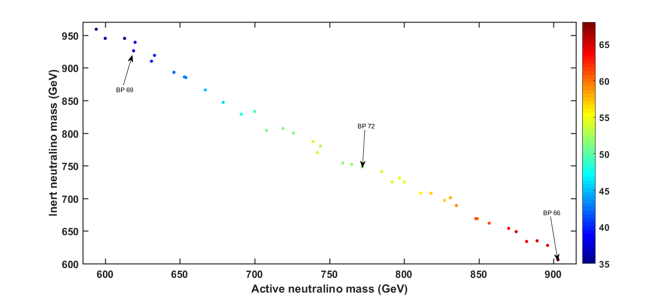

In our scan we have kept the other particles so heavy that resonant annihilation does not occur. If, however, it happened to be that one of the DM candidates had a mass close to, say, , the resonant annihilation could give the correct relic density in a configuration that would otherwise lead to overabundance. For further examination, we pick Benchmark Points (BPs) with neutralino masses given in Tab. 2. One of the BPs has a heavy active and a light inert higgsino, one has a heavy inert and a light active higgsino and one has roughly degenerate DM candidates. For all of the BPs we have TeV, which is the experimental lower bound in our case.
| Benchmark | Active mass | Inert mass | ||
|---|---|---|---|---|
| BP66 | ||||
| BP69 | ||||
| BP72 |
We show the relic densities of the individual higgsino components for the points satisfying the relic density constraint as a function of their masses in Fig. 3. There is a small difference in the relic density, which is due to the larger Boltzmann suppression (the mass splittings are larger) in the case of the active higgsino, which reduces the neutralino-chargino coannihilation rate. We can also see that the heavier component has a slightly smaller relic density than it would have had in a single DM component scenario. This is due to charged current interactions, where the lighter chargino scatters from the heavier neutralino and produces a heavy chargino and a light neutralino and the heavy chargino then annihilates a heavy neutralino. This charged current process is more efficient when the colliding particles have a similar mass so that the lab frame is close to the center-of-mass frame. For SM particles the situation would be close to a fixed target scattering, where the threshold energy for chargino production is larger.
This process also explains why the sum of masses is slightly different for different mass orderings. The mass splitting between the active chargino and active neutralino is larger so that is always kinematically allowed whereas there is a threshold for the process . Hence the effect of the lighter DM component is larger in the case when the active one is lighter and hence the sum of masses also is.

The annihilation proceeds mostly through the SM gauge bosons either as neutralino-neutralino annihilation through the boson or as neutralino-chargino coannihilation through the so the annihilation cross section is almost completely insensitive to scanning parameters besides the higgsino masses. The only other annihilation channel that could contribute is via a Higgs boson through the Superpotential coupling , but that only contributes through the singlino component of the higgsino, which is always tiny. Furthermore, the coupling is , i.e., clearly smaller than the gauge couplings. Hence, a Higgs mediated contribution is always below the percent level.
The scenario with two higgsinos is also viable from the viewpoint of DD bounds. As we discuss in the next section, the Spin-Independent (SI) cross section for the active higgsino is about an order of magnitude below the limits from Xenon1T Aprile2018 while for the inert higgsino the scattering cross section is a couple of orders smaller than for the active one. Also the Spin-Dependent (SD) cross section is larger for the active higgsino.
III.2 Wino and inert higgsino as DM candidates
The wino as a DM candidate leads to underabundance of relic DM, if it is lighter than TeV Profumo2004. However, together with the inert higgsino, one may achieve the correct relic density. Also in this case the annihilations are basically independent. Due to the more efficient annihilation process of the wino, the masses of the two neutralinos need to be larger than in the case of two higgsinos. Typically, the wino needs to be twice as heavy as the higgsino to get the same relic density. The wino component gives roughly of the relic density when the two DM candidates are degenerate, which happens around GeV.
As the abundance of the wino component is smaller and it couples to the boson only through its mixing with the higgsinos, this scenario will be harder to discover through DD experiments. The SI DD cross section pb, which might eventually be detectable (as we shall se below). As the case with two higgsinos has the higher chance for detection, we shall concentrate on it in the following.
III.3 Other combinations
None of the other scenarios produces a viable pair of DM candidates. In the inert sector the inert doublet scalars have too large a DD cross section, which rules these out. The inert singlets have masses of the order of the mass and hence they are never the lightest particles in the inert sector. Finally, also the non-MSSM gaugino has a mass of the order of the mass and hence it will not be the lightest Superpartner while the usual bino leads to overabundance without resonant annihilation.
IV Two Higgsinos DM and Direct Detection Experiments
We now discuss the SI and SD DM scattering cross section of the active and inert higgsino DM that we discussed in the previous section. The relevant Feynman diagrams for DD are given in Fig. 4.

The effective scalar interactions of these two DM candidates with up and down quarks are mainly given by exchange and the interaction with gluons is induced by Higgs exchange through heavy-quark loops, i.e.,
| (19) |
where comes from the mediated process and is Higgs-gluon coupling induced by the heavy quark loops. The effective coupling of with protons and neutrons , can be computed in terms of , and Jungman1996 with the zero momentum transfer scalar cross section of the higgsino scattering with the nucleus given by Belanger2009:
| (20) |
where and are the number of protons and neutrons, respectively, , where is the nucleus mass. Thus, the differential scalar cross section for non-zero momentum transfer can be written as
| (21) |
where is the velocity of the lightest neutralino and is the relevant Form Factor (FF) Jungman1996. Therefore, the SI (scattering) cross section of the LSP with a proton is given by
| (22) |
The SD interaction of a DM candidate stems solely from the quark axial current:
where , with the effective quark level axial-vector and pseudoscalar couplings and is given via , , and . In this case, the SD (scattering) cross section of DM-nucleus is given by
| (23) |
where is the angular momentum of the target nucleus. In case of the proton target, .
In Fig. 5, we display the SI and SD cross sections of the active (left panel) and inert (right panel) higgsino LSP with a proton after imposing the relic abundance constraints. As the DM-nucleon recoil rates are dependent on the local density of the DM candidate, in the case of multicomponent DM the density of each species is smaller and then it is necessary to re-scale the factor, where is the relic abundance for the active () or the inert () neutralino. All our BPs satisfy the XENON-1T exclusion region and, in the case of SI interactions, the active DM candidate is clearly within the region of visibility for future DD experiments like XENON-nT and DARWIN Aalbers2016. However, the cross section of the inert higgsino is too low and therefore falls into the neutrino floor or neutrino coherent scattering Baudis2014, where it will be challenging to probe in the future. We have highlighted the exemplary BPs 66 (orange), 69 (blue) and 72 (navy).
The differences between the active and inert neutralinos can be understood rather easily. In the SD case the higgsino coupling to the boson comes from
| (24) |
where and give the and components of the lightest neutralino. If the mass matrix had only the -term, then and the coupling would vanish. Since the active higgsinos mix with the gauginos, and hence the coupling is non-zero, while for inert higgsinos the coupling vanishes as they do not mix with other states. When gauge kinetic mixing is introduced, also the inert higgsino gets a coupling to the boson but this is much smaller than that of the active higgsino.
The difference in the SI cross section arises from the SM-like Higgs mediated scattering, which again is only relevant for the active higgsino as it mixes with the singlino. The SI cross section of the inert higgsino arises through the , the active singlet (which are heavy) or the tiny singlet-doublet mixing of the SM-like Higgs. Also, the squarks can act as mediators in the case of an active higgsino, but their contribution is so small that it can be neglected. For the inert higgsino the is the only mediator with unsuppressed couplings. For the channel the coupling is suppressed by the small kinetic mixing and for scalar mediators by the even smaller singlet-doublet mixing. As mentioned before, for these BPs, we have taken TeV and used . The DD cross sections arising from for other masses and couplings will scale as .
In the case of SI interactions, the distribution of the number of events versus the recoil energy can be calculated as
| (25) |
where is the DM density near the Earth, the mass of the detector, the exposure time and the nucleus FF which depends on the momentum transfer and
| (26) | |||||
| (27) |
where is the mass of the nucleus.
For SI interactions, the FF is a Fourier transform of the nucleus distribution function,
| (28) |
where is normalised such that . In micrOMEGAs Belanger2009, the Fermi distribution function is used:
| (29) |
where the normalisation condition fixes , and fm for a surface thickness fm.
In the case of SD interactions, instead of the nuclear FF one needs to introduce instead the coefficients , and , which are the nuclear structure functions that take into account both the magnitude of the spin in the nucleon and the spatial distribution of it. Then, the number of events over the nucleus recoil energy is
| (30) |
where the SD FFs are described using a Gaussian distribution:
| (31) |
where fm.
The normalisation of and the list of all SD FFs implemented in micrOMEGAs can be consulted in Belanger2009.
In Fig. 6 we show the event rate for DD of active higgsinos (purple) and inert higgsinos (green) as a function of the recoil energy of the nucleus for different dectection materials: Xe, Ge, Na and Si. The rate is multiplied by the WIMP mass to make the curves on the plot independent of the neutralino mass. This recoil energy can be split in its SI and SD parts. As the SI part for the inert DM candidate is much lower than the SD part (in comparison with the active DM candidate), the total shape for both DM candidates is different. The expected sensitivity for experiments using Ge, Na or Si is not low enough for our DM candidates to be seen in these cases Akerib2010. For Xe, it is different. Thus, in the top three frames of Fig. 7, we show the expected sensitivity to see the DM candidates in BPs 66, 69 and 72 in the case of liquid Xe experiments, wherein we have a background that includes the electron recoil spectrum from the double-beta decay of 136Xe () and the summed differential energy for and 7Be neutrinos (Be) undergoing neutrino-electron scattering. To discriminate between Nuclear Recoil (NR) and Electronic Recoil (ER) or background, liquid Xe experiments split the signal in two regions, S1 and S2, which respond differently to such recoils Cushman2013. In here, a 99.98% discrimination of ERs at 30% NR acceptance is assumed and the recoil energies are derived using the S1 signal only, according to Refs. Aalbers2016; Baudis2014. Finally, in the three bottom frames of Fig. 7, we show the ratio of the rates for total signal (alongside that of the active neutralino only) and background. Specifically, the total signal rate corresponds to the addition of the SI and SD event rates of both the active and inert higgsino while the background rate corresponds to the addition of the neutrino rates from double beta decay and scattering. The total number of events corresponding to our DM candidates is up to times larger that the number of events with neutrinos for low recoil energies and up to ten times larger for recoil energies larger that 100 keV, thus clearly vouching for a forthcoming (potential) discovery of the active neutralino component of DM. Furthermore, the difference in shape between the latter and the total signal for recoil energies below 60 keV may offer a hint of the presence of a second DM component, so long that a significant level of control can be achieved on the shapes of both the dominant DM signal and the background.
V Two Higgsinos DM and Indirect Detection Experiments
| BP | mass (GeV) | |||
|---|---|---|---|---|
| 66 (active) | 903 | |||
| 66 (inert) | 606 | |||
| 69 (active) | 619 | |||
| 66 (inert) | 926 | |||
| 72 (active) | 766 | |||
| 72 (inert) | 753 |
One of the most important methods for detecting DM in the galactic halo is the observation of -rays emitted from the DM annihilation at the galactic center. The differential spectrum of the total observed -ray flux is given by
| (32) |
where is the differential -ray flux generated from the DM, defined as
| (33) |
where is the -ray spectrum produced per annihilation and the astrophysical factor of Eq. (33) can be identified as
| (34) |
For generalised Navarro-Frenk-White (NFW) halo profile with inner slope , one finds that the astrophysical factor is of order GeV2 cm-5 Daylan2016; Calore2015. Finally, is the isotropic -ray backgrounds Abdo2010. In Tab. 3 we give the values of for each of the active and inert higgsinos of our selected BPs.
In Fig. 8, we show the differential flux of -ray secondary radiation from the galactic center as a function of the photon energy. We show the -ray spectrum produced by the three exemplary BPs 66, 69 and 72 for both the active (purple) and inert (green) neutralino. The FermiLAT data (with error) are presented in black and the corresponding distribution for the background is shown in red. The distributions are very dependent on the masses and the flux is larger the lighter the mass of the higgsino. In contrast with DD experiments, when the inert neutralino is the lightest it would be this the DM candidate giving the largest contribution to the photon flux.
The -ray flux can be evaluated as
| (35) |
and is expressed in number of photons per cm2 per s per sr. The factor includes the integral of the squared of the DM density over the line of sight,
| (36) |
where and being the angle of observation, the distance from the Sun to the galactic center.
Another two interesting astrophysical probes to analyse with DM candidates are the antiproton and positron excesses reported by PAMELA Galper2018 and AMS-02 Aguilar2016. The propagation of charged particles in Cosmic Rays (CRs) is one of the largest sources of uncertainties in predicting the background of antiprotons or positrons and the signal from DM annihilation Belanger2011; Aguilar2016; Cui2018; Donato2004. Charged particles are deflected by a diffusion process in the random galactic magnetic field. The equation that describes the evolution of the energy distribution is
| (37) |
where is the number density of particles per unit volume and energy, denotes the particle species, is the source term and the energy loss rate. For antiprotons there is an extra term which accounts for a negative contribution to the source term, as we explain below. Further, is the space diffusion coefficient, assumed homogeneous:
| (38) |
where is the particle velocity and its rigidity. The collision between primary nuclei and the interstellar gas leads to fragmentation of the parent nuclei and the production of secondary nuclei. Therefore the secondary-to-primary particle ratio, e.g., the Boron-to-Carbon (B/C) ratio, is usually employed to constrain the propagation parameters Maurin2001; Feng2016; Cui2018. The coefficient introduced above is adequate to fit this B/C data.
In the case of positrons flux, the loss rate is dominated by synchrothon radiation in the galactic magnetic field and inverse Compton scattering on stellar light and CMB photons, so that it is defined by
| (39) |
where s is the typical energy loss time. Then the positron flux from DM annihilation reads as
| (40) |
where is a universal function for all energies. In MicrOMEGAs, the routine posiFluxTab tabulates first as a function of in the region and then perfom a fast integration for all energies.
In the case of antiprotons, the propagation is dominated by diffusion and the effect of the galactic wind. As stated above, for antiprotons it is needed to add to Eq. (37) a negative source, which corresponds to the fragmentation or decay of antiprotons in the interstellar medium . The annihilation rate is
| (41) |
where is the velocity of the antiproton, cm-3 and cm-3 are the average densities in the galactic disc while is the annihilation cross section that can be found in Ref. Belanger2011; Tan1982. (The production of the secondary antiprotons is not included in the MicrOMEGAs code.)
Afer integration, the antiproton energy spectrum is
| (42) |
with and where is the Green function which determines the probability of a CR to propagate from the source to the detector, as defined in Ref. Belanger2011.
In Figs. 9 and 10 we show the resulting fluxes for positron and antiproton production, respectively. For both cases we are comparing with the recent AMS-02 data Aguilar2019. In the case of the positron flux, the data reported by AMS-02 seems compatible with the background (given by a diffused flux which corresponds to the observations of positrons before the last AMS-02 report Queiroz2020) at low energies, but it requires a new source to explain the flux at higher energies. Unfortunately, both the active and inert higgsinos have a shape similar to the background and fail in proving a source to explain the excess at energies above 10 GeV. In the case of the antiproton flux, the background corresponds to inelastic collisions between protons and the interstellar medium Cui2018. The data of AMS-02 fits very well with the background, although there is room to improve the fit for energies between 10 to 100 GeV. However, a better explanation to this excess would correspond to a DM candidate of lighter mass than the active and inert higgsinos of the E6SSM.
VI Conclusions
We have analysed the possibility of having two-component DM in a simplified version of a SUSY GUT model, the E6SSM, which is inspired by string theory. We have shown that one of these DM components is the lightest active neutralino (higgsino-like) that has direct couplings to the SM fermions. The other DM component is the lightest inert neutralino (also higgsino-like) that does not have a direct interaction with the SM fermions, however, it couples to the gauge bosons as it is originating from the inert Higgs doublets. These two particles are stable, hence, they are candidates for DM, because of the -parity and symmetries to which they obey, respectively.
We have then emphasised that the relic abundance limit implies that the sum of the masses of these two DM components is nearly constant and of order TeV. We have thus considered three BPs that give comparable contributions to from each DM component. In particular, we have studied the following cases: , and . We have first investigated the DD of these three cases. In particular, we have considered the SI and SD cross sections of these two DM components and compared their results with current and future experimental measurements. We have shown that the active higgsino is within the future XENON-nT and DARWIN sensitivity, however, the inert higgsino cross sections are generally too low, which make its identification extremely difficult, though not altogether impossible. In addition, we have studied the nuclear recoil energy associated with the two DM components while interacting detector materials: Xe, Ge, Na and Si. Here, we have shown that, again, for future Xe detectors, the active higgsino results can be well above the background (especially at low energies), hence, that this DM component has a chance to be probed in future DD experiments also for the purpose of extracting its mass. In contrast, the inert higgsino contributions are quite small and lower than the background, although this DM candidate may become evident in the recoil distribution of Xe experiments for significant exposures, when both the background and other DM signal will be known more accurately, in the form of a modifiation to the dominant signal shape (at small to intermediate recoil energies). Finally, we have analysed the ID rates, through -ray spectra as well as positron and antiproton fluxes, for both active and inert higgsinos. In this case, we have found that all results stemming from active DM dynamics are well below the current limits and the inert DM predictions are extremely small in comparisons, so that we have concluded that sensitivity here will be minimal for years to come.
Acknowledgements
DR-C is supported by the Royal Society Newton International Fellowship NIF/R1/180813. SK acknowledges partial support from the Durham IPPP Visiting Academics (DIVA) programme. SM is financed in part through the NExT Institute and the STFC consolidated Grant No. ST/L000296/1. HW acknowledges financial support from the Magnus Ehrnrooth Foundation and STFC Rutherford International Fellowship (funded through the MSCA-COFUND-FP Grant No. 665593). We would like to thank Yasar Hiciylmaz for helpful discussions and for providing the code to produce Figure 6. The authors acknowledge the use of the IRIDIS High Performance Computing Facility, and associated support services at the University of Southampton, in the completion of this work.
References
- (1) Planck collaboration, Planck2015 results, Astronomy & Astrophysics 594 (2016) A13 [1502.01589].
- (2) Planck collaboration, Planck 2018 results. VI. Cosmological parameters, 1807.06209.
- (3) L. Wang, V. Gonzalez-Perez, L. Xie, A.P. Cooper, C.S. Frenk, L. Gao et al., The galaxy population in cold and warm dark matter cosmologies, Monthly Notices of the Royal Astronomical Society 468 (2017) 4579 [1612.04540].
- (4) S. Khalil and S. Moretti, Supersymmetry Beyond Minimality, Taylor & Francis Ltd (2019).
- (5) S.F. King, S. Moretti and R. Nevzorov, Theory and phenomenology of an exceptional supersymmetric standard model, Physical Review D 73 (2006) 035009 [hep-ph/0510419].
- (6) S. King, S. Moretti and R. Nevzorov, Exceptional supersymmetric standard model, Physics Letters B 634 (2006) 278 [hep-ph/0511256].
- (7) S.F. King, S. Moretti and R. Nevzorov, A Review of the Exceptional Supersymmetric Standard Model, Symmetry 12 (2020) 557 [2002.02788].
- (8) P. Athron, S.F. King, D.J. Miller, S. Moretti and R. Nevzorov, The Constrained Exceptional Supersymmetric Standard Model, Phys. Rev. D 80 (2009) 035009 [0904.2169].
- (9) P. Athron, S. King, D. Miller, S. Moretti and R. Nevzorov, Predictions of the Constrained Exceptional Supersymmetric Standard Model, Physics Letters B 681 (2009) 448 [0901.1192].
- (10) P. Athron, S.F. King, D.J. Miller, S. Moretti and R. Nevzorov, LHC signatures of the constrained exceptional supersymmetric standard model, Physical Review D 84 (2011) 055006 [1102.4363].
- (11) P. Athron, S.F. King, D.J. Miller, S. Moretti and R. Nevzorov, Constrained exceptional supersymmetric standard model with a higgs signal near 125 GeV, Physical Review D 86 (2012) 095003 [1206.5028].
- (12) P. Athron, D. Harries, R. Nevzorov and A.G. Williams, Inspired SUSY benchmarks, dark matter relic density and a 125 GeV Higgs, Physics Letters B 760 (2016) 19 [1512.07040].
- (13) P. Athron, A. Thomas, S. Underwood and M. White, Dark matter candidates in the constrained Exceptional Supersymmetric Standard Model, Physical Review D 95 (2017) 035023 [1611.05966].
- (14) J.P. Hall and S.F. King, Bino Dark Matter and Big Bang Nucleosynthesis in the Constrained SSM with Massless Inert Singlinos, JHEP 06 (2011) 006 [1104.2259].
- (15) J.P. Hall and S.F. King, Neutralino dark matter with inert higgsinos and singlinos, Journal of High Energy Physics 2009 (2009) 088 [0905.2696].
- (16) F. del Aguila, G. Coughlan and M. Quiros, Gauge Coupling Renormalization With Several U(1) Factors, Nucl. Phys. B 307 (1988) 633.
- (17) F. del Aguila, J. Gonzalez and M. Quiros, Renormalization Group Analysis of Extended Electroweak Models From the Heterotic String, Nucl. Phys. B 307 (1988) 571.
- (18) E. Accomando, D. Becciolini, A. Belyaev, S. Moretti and C. Shepherd-Themistocleous, Z at the LHC: interference and finite width effects in drell-yan, Journal of High Energy Physics 2013 (2013) 153 [1304.6700].
- (19) E. Accomando, F. Coradeschi, T. Cridge, J. Fiaschi, F. Hautmann, S. Moretti et al., Production of z-boson resonances with large width at the LHC, Physics Letters B 803 (2020) 135293 [1910.13759].
- (20) ATLAS collaboration, Search for high-mass dilepton resonances using 139 fb-1 of collision data collected at 13 tev with the atlas detector, Phys. Lett. B 796 (2019) 68 [1903.06248].
- (21) M. Frank, Y. Hiçyılmaz, S. Moretti and O. Ozdal, E6 motivated UMSSM confronts experimental data, Journal of High Energy Physics 2020 (2020) 123 [2004.01415].
- (22) S. Profumo and C.E. Yaguna, Statistical analysis of supersymmetric dark matter in the minimal supersymmetric standard model after WMAP, Physical Review D 70 (2004) 095004 [hep-ph/0407036].
- (23) L. Randall and R. Sundrum, Out of this world supersymmetry breaking, Nuclear Physics B 557 (1999) 79 [hep-th/9810155].
- (24) S. Bhattacharya, A. Drozd, B. Grzadkowski and J. Wudka, Two-Component Dark Matter, JHEP 10 (2013) 158 [1309.2986].
- (25) F. Staub, SARAH 4 : A tool for (not only SUSY) model builders, Comput. Phys. Commun. 185 (2014) 1773 [1309.7223].
- (26) W. Porod and F. Staub, SPheno 3.1: extensions including flavour, CP-phases and models beyond the MSSM, Computer Physics Communications 183 (2012) 2458 [1104.1573].
- (27) G. Belanger, F. Boudjema, A. Pukhov and A. Semenov, micrOMEGAs: A Tool for dark matter studies, Il Nuovo Cimento C 33 (2010) 111 [1005.4133].
- (28) G. Bélanger, F. Boudjema, A. Pukhov and A. Semenov, micrOMEGAs4.1: Two dark matter candidates, Computer Physics Communications 192 (2015) 322 [1407.6129].
- (29) XENON collaboration, Dark Matter Search Results from a One Ton-Year Exposure of XENON1T, Phys. Rev. Lett. 121 (2018) 111302 [1805.12562].
- (30) G. Jungman, M. Kamionkowski and K. Griest, Supersymmetric dark matter, Physics Reports 267 (1996) 195 [hep-ph/9506380].
- (31) G. Bélanger, F. Boudjema, A. Pukhov and A. Semenov, Dark matter direct detection rate in a generic model with micrOMEGAs_2.2, Computer Physics Communications 180 (2009) 747 [0803.2360].
- (32) DARWIN collaboration, DARWIN: towards the ultimate dark matter detector, JCAP 11 (2016) 017 [1606.07001].
- (33) L. Baudis, A. Ferella, A. Kish, A. Manalaysay, T. Marrodan Undagoitia and M. Schumann, Neutrino physics with multi-ton scale liquid xenon detectors, JCAP 01 (2014) 044 [1309.7024].
- (34) CDMS collaboration, A Low-Threshold Analysis of CDMS Shallow-Site Data, Phys. Rev. D 82 (2010) 122004 [1010.4290].
- (35) P. Cushman et al., Working Group Report: WIMP Dark Matter Direct Detection, in Community Summer Study 2013: Snowmass on the Mississippi, 10, 2013 [1310.8327].
- (36) T. Daylan, D.P. Finkbeiner, D. Hooper, T. Linden, S.K.N. Portillo, N.L. Rodd et al., The characterization of the gamma-ray signal from the central Milky Way: A case for annihilating dark matter, Phys. Dark Univ. 12 (2016) 1 [1402.6703].
- (37) F. Calore, I. Cholis and C. Weniger, Background Model Systematics for the Fermi GeV Excess, JCAP 03 (2015) 038 [1409.0042].
- (38) Fermi-LAT collaboration, The Spectrum of the Isotropic Diffuse Gamma-Ray Emission Derived From First-Year Fermi Large Area Telescope Data, Phys. Rev. Lett. 104 (2010) 101101 [1002.3603].
- (39) PAMELA collaboration, Ten years of CR physics with PAMELA, Adv. Space Res. 62 (2018) 2892.
- (40) AMS collaboration, Antiproton Flux, Antiproton-to-Proton Flux Ratio, and Properties of Elementary Particle Fluxes in Primary Cosmic Rays Measured with the Alpha Magnetic Spectrometer on the International Space Station, Phys. Rev. Lett. 117 (2016) 091103.
- (41) G. Belanger, F. Boudjema, P. Brun, A. Pukhov, S. Rosier-Lees, P. Salati et al., Indirect search for dark matter with micrOMEGAs2.4, Comput. Phys. Commun. 182 (2011) 842 [1004.1092].
- (42) M.-Y. Cui, X. Pan, Q. Yuan, Y.-Z. Fan and H.-S. Zong, Revisit of cosmic ray antiprotons from dark matter annihilation with updated constraints on the background model from AMS-02 and collider data, Journal of Cosmology and Astroparticle Physics 2018 (2018) 024 [1803.02163].
- (43) F. Donato, N. Fornengo, D. Maurin and P. Salati, Antiprotons in cosmic rays from neutralino annihilation, Phys. Rev. D 69 (2004) 063501 [astro-ph/0306207].
- (44) D. Maurin, F. Donato, R. Taillet and P. Salati, Cosmic rays below z=30 in a diffusion model: new constraints on propagation parameters, Astrophys. J. 555 (2001) 585 [astro-ph/0101231].
- (45) J. Feng, N. Tomassetti and A. Oliva, Bayesian analysis of spatial-dependent cosmic-ray propagation: astrophysical background of antiprotons and positrons, Phys. Rev. D 94 (2016) 123007 [1610.06182].
- (46) L. Tan and L. Ng, Parametrization of anti-p invariant cross-section in pp-collisions using a new scaling variable, Phys. Rev. D 26 (1982) 1179.
- (47) AMS collaboration, Towards Understanding the Origin of Cosmic-Ray Positrons, Phys. Rev. Lett. 122 (2019) 041102.
- (48) F.S. Queiroz and C. Siqueira, Explaining the AMS positron excess via Right-handed Neutrinos, Phys. Rev. D 101 (2020) 075007 [1910.04782].
- (49) L.D. Rose, S. Khalil, S.J.D. King, S. Kulkarni, C. Marzo, S. Moretti et al., Sneutrino Dark Matter in the BLSSM, Journal of High Energy Physics 2018 (2018) 100 [1712.05232].