Emergence, Non-equilibrium statistical physics
David H. Wolpert
Strengthened second law for multi-dimensional systems coupled to multiple thermodynamic reservoirs
Abstract
The second law of thermodynamics can be formulated as a restriction on the evolution of the entropy of any system undergoing Markovian dynamics. Here I show that this form of the second law is strengthened for multi-dimensional, complex systems, coupled to multiple thermodynamic reservoirs, if we have a set of a priori constraints restricting how the dynamics of each coordinate can depend on the other coordinates. As an example, this strengthened second law (SSL) applies to complex systems composed of multiple physically separated, co-evolving subsystems, each identified as a coordinate of the overall system. In this example, the constraints concern how the dynamics of some subsystems are allowed to depend on the states of the other subsystems. Importantly the SSL applies to such complex systems even if some of its subsystems can change state simultaneously, which is prohibited in a multipartite process. The SSL also strengthens previously derived bounds on how much work can be extracted from a system using feedback control, if the system is multi-dimensional. Importantly, the SSL does not require local detailed balance. So it potentially applies to complex systems ranging from interacting economic agents to co-evolving biological species.
keywords
Stochastic thermodynamics, Multi-dimensional systems, Multipartite processes, Entropy production, Feedback control, Second law of Thermodynamics, complex systems1 Introduction
Statistical physics concerns experimental scenarios where we have restricted information concerning the state of a system , which is quantified as a probability distribution over those states, . In particular, the recently developed variant of statistical physics called “stochastic thermodynamics” concentrates on systems that evolve according to a continuous time Markov chain (CTMC). For a countable state space, this means that evolves according to a linear differential equation,
| (1) |
(Note that the rate matrix can depend on time .)
Analyzing systems which evolve according to Eq. 1 has led to formulations of the second law of thermodynamics which apply even if the system is evolving while arbitrarily far out of thermal equilibrium [42, 35]. If we apply one of these formulations of the second law to any system evolving according to Eq. 1 while coupled to a single (infinite) heat bath at temperature , and assume that the rate matrix is related to an underlying Hamiltonian via local detailed balance (LDB), we get
| (2) |
where is the total heat flow into the system from its heat bath during the dynamics, and is the change in Shannon entropy of the system during the process.
If LDB does not hold, Eq. 2 will not hold either, if we wish to interpret as thermodynamic heat flow. However, for any rate matrix, regardless of whether it obeys LDB,
| (3) |
(for a process lasting from time to ). The quantity on the LHS of Eq. 3 is called the total expected entropy flow (EF) into the system during the process. The difference between the entropy change of the system (the RHS of Eq. 3) and the EF is called the entropy production (EP), written as . So Eq. 3 can be re-expressed as
| (4) |
Crucially, the inequality Eq. 4 holds for any CTMC, even a CTMC that has no thermodynamic interpretation, i.e., a CTMC which models a process that does not involve energy transduction. So Eq. 4 applies to dynamic models of everything from stock markets to the evolution of the joint state of an opinion network, so long as those models are CTMCs.
In many experimental scenarios, while we are restricted in the information we have concerning the system’s state, we also have some other information that does not directly concern the system’s state, in the form of conditions satisfied by the dynamics of the system. Recently Eq. 4 has been strengthened, by adding non-positive terms to the RHS that incorporate this kind of information concerning the dynamics. Examples of these new results include “thermodynamic uncertainty relations” (TURs [15, 23, 21, 9]), “speed limit theorems” (SLTs [36, 50, 28, 43, 11]), “thermodynamic first passage bounds” [27, 10, 8, 30, 26], etc.
Unlike Eq. 4 though, these bounds require measuring variables as they change during the process, in addition to knowing the beginning and ending distributions, and . (For example, TURs rely on measuring accumulated currents, and speed limit theorems rely on measuring integrated activity.) This limits their experimental applicability.
In this paper, I derive new strengthened forms of Eq. 4 that, like the TURs and speed limit theorems, incorporate information concerning the dynamics of the system. However, unlike the TURs, speed limit theorems, etc., these new strengthened forms of Eq. 4 do not require measuring variables as they change during the process.
These strengthened forms of Eq. 4 apply whenever we have information about which of the coordinates of the system can have their dynamics directly depend on which of the other coordinates. Formally, such information takes the form of constraints on the rate matrix of the CTMC governing the dynamics of the system. (See also [20].) I call this kind of restriction on the allowed dynamics a “dependency constraint”.

As an example, consider a random walker over a two-dimensional finite lattice, . For simplicity take for two positive integers . The lattice is coarse-grained into a set of non-overlapping squares each of size , and the position of the walker in the lattice is represented three-dimensionally, by a pair of coordinates and an integer . (The value specifies the precise coarse-grained square, while specifies the coordinates within that square.) In addition to position in the lattice, the walker has internal stores of two nutrients, and , specified (up to some coarse-graining) by values in the finite sets and and , respectively. So the state space of the walker is , i.e., those five variables are the five coordinates of the walker.
We can suppose that both and evolve autonomously, independently of all other variables, according to two associated rate matrices, i.e., the walker engages in two independent random walks, one in each of the two directions across the lattice. Note though that ’s dynamics will depend on and in general, and that there will sometimes be simultaneous transitions of and some other coordinate. For example, suppose , so the walker is at the extreme value of within some square, adjacent to the next coarse-grained square. Suppose as well that in the next step, the walker moves into that adjacent square. So simultaneously changes to while must also change, since the coarse-grained square changes. However, for other changes in , remains unchanged.
We can also suppose that the dynamics of depends only on the walker’s current position in and their current amount of , i.e., it depends only on . Similarly, the dynamics of depends only on . (For example, this would be the case if densities of those two nutrients were arranged appropriately across the lattice, and the walker at a given location accumulates those nutrients based on their densities at that location.) Summarizing, the dependency constraints are that depends only on (in addition to depending on its own state), depends only on (in addition to its own state), and are autonomous, while can depend on and / or (in addition to itself).
There are many other dynamic processes over a state space which obey a set of dependency constraints among the coordinates of the state space, but those coordinates do not specify characteristics of a single agent like a walker traversing a lattice. For this special issue on the topic of ‘Emergence’, perhaps the most important type of system that evolves subject to dependency constraints is a system that comprises a set of physically separated subsystems, co-evolving with one another, with each subsystem’s state being identified as a different coordinate [16, 47, 46]. In this kind of system, dependency constraints governing the dynamics of each coordinate, specifying which other coordinates can directly affect its dynamics, amount to constraints on the dynamics of each subsystem, specifying which other subsystems can directly affect its dynamics. As a concrete illustration, consider the scenario investigated in [13, 2], in which receptors in the wall of a cell sense the concentration of a ligand in the intercellular medium, and those receptors are in turn observed by a “memory” subsystem inside the cell. Modify this scenario by introducing a second cell, which is observing the same external medium as the first cell. Assume that the cells are far enough apart physically so that their dynamics are independent of one another. This gives us the precise scenario in Fig. 1, where subsystem is concentration in the external medium, subsystem is the state of the receptors of the first cell, subsystem is the memory subsystem of the first cell, and subsystem is the state of the receptors of the second cell.
In this paper I consider how a set of dependency constraints on an evolving system affect its thermodynamics. My main result shows how such a set of dependency constraints can strengthen Eq. 4, by adding an expression to its RHS. This expression involves only those dependency constraints and the starting and ending distribution of the system. As a caveat, this new lower bound on EP is not always positive, i.e., it is not always stronger than the conventional second law, Eq. 4. However, I show below that for any set of dependency constraints, there is a conditional distribution that can be implemented by a rate matrix obeying those constraints, together with an initial distribution , such that every rate matrix that implements that conditional distribution must result in a non-negative EP when applied to that initial distribution. Indeed, for some sets of dependency constraints, this new EP bound is stronger than the conventional second law no matter what and are (so long as is consistent with the dependency constraints).
Some of the TURs, SLTs, etc., rely on the dynamics obeying LDB. LDB is not required for the new extension of the second law derived here. This means that (for example) this new extension applies to multipartite systems that have “directed” (sometimes called “non-reciprocal”) interactions rather than undirected interactions among the subsystems, i.e., interactions in which there is exactly zero back-action [12, 13, 31, 29, 44, 22, 34, 24]. Very often, these systems violate strict LDB, and so their thermodynamic analyses are, at best, approximations. (See discussion in appendix in [46] of some conditions that justify this approximation.) In contrast, the result derived below applies exactly to any scenario where there is no back-action, with no approximation. In addition, this result holds even if the dynamics allows multiple coordinates to change simultaneously. In particular, in the special case that each coordinate is a separate subsystem, the result does not require that the dynamics be a multipartite process [16].
Due to these relaxations of the assumptions made in conventional stochastic thermodynamics, the results below are not restricted to thermodynamic systems, involving energy transduction. The results hold for any CTMC, even if the rate matrix does not reflect physically coupling between the system and one or more external thermodynamic reservoirs, as it does in conventional applications of stochastic thermodynamics [42].
However, the strengthened second law derived below has special physical significance in the common scenario where the dependency constraints arise because the system’s dynamics is governed by coupling with external reservoirs, and there are restrictions on that coupling. For example, a common physical scenario is where the system has multiple subsystems, and each subsystem is coupled to a physically distinct part of a shared reservoir. Due to the physical separation of those parts of the reservoir, each connected to a different subsystem, the usual assumption of time-scale separation between the dynamics of the overall system and that of the reservoirs means that the different subsystems are effectively coupled to independent reservoirs from one another.11 1 It is important to note that this separation is between the time-scale of the dynamics of the overall system and the time-scale of the implicit dynamics of the thermodynamic reservoirs that are coupled to the system [35]. It does not concern the time-scales of the dynamics of the different coordinates of the system. For analysis of the latter kind of time-scale separation in the special case of a bipartite system, see [5], and for a more general analysis, see [39]. Such systems evolve as a multipartite process (MPP), in which no transitions are allowed in which more than two subsystems change their states exactly simultaneously [16]. If the system is an MPP, and the dynamics of each subsystem obeys LDB, then we can use stochastic thermodynamics to identify various attributes of that dynamics with experimentally measurable thermodynamic quantities [17, 16, 12, 1, 4]. More generally, there are systems with multiple coordinates that aren’t usually viewed as separate “subsystems”, but where the global dynamics arises due to the system’s coupling with thermodynamic reservoirs, and where each reservoir is only coupled to a single coordinate. These systems can also be modeled as MPPs, and analyzed accordingly.
Generalizing further, there are other kinds of systems that also have multiple coordinates, where the global dynamics arises due to the system’s coupling with thermodynamic reservoirs, just like in an MPP. Also like in an MPP, each reservoir in these systems is only coupled to a proper subset of the coordinates, which results in dependency constraints. In contrast to an MPP however, some reservoirs are coupled to more than one coordinate. As an example, as stated in [6]: “Fluctuations in biochemical networks, e.g. in a living cell, have a complex origin that precludes a description of such systems in terms of bipartite or multipartite processes, as is usually done in the framework of stochastic and/or information thermodynamics.” The strengthened second law I present below applies to these generalized forms of MPPs as well as to MPPs.
In the next section I formalize dependency constraints as restrictions on the rate matrix of a CTMC. This is followed by a section in which I use this formalization to derive an expression for the EP of system that involves the triple of {the rate matrix dependency constraints, the initial distribution over states, the final distribution over states}, together with certain other factors. In the following section I derive a lower bound on that expression for EP which depends only on the triple of {dependency constraints, initial distribution, final distribution}, without those other factors. In particular, this lower bound does not depend on any properties of the rate matrix, other than the dependency constraints. This lower bound is my main result. In the following section this main result to analyze how the thermodynamics of feedback control [31, 29, 20] changes when we know that the system being controlled obeys a given set of dependency constraints. In the following section I present a set of examples of my main result. I end with some discussion, in particular of the relation of the new result to other results in the literature.
2 Rate matrix unit structures
I begin by defining notation. First, I write the state space of the system as , where each finite state space is a coordinate of the system. I write the set of coordinates as . As examples, each coordinate could specify the state of a physically separate subsystem of the overall system, or it could specify a position on one axis of a lattice, or it could indicate a degree of freedom in a multi-scale specification of the state of the system.
The distribution over the states of the system is assumed to evolve according to a continuous time Markov chain (CTMC)22 2 Note that assuming the state space of the system is a Cartesian product does not limit the applicability of the analysis. Suppose that the set of physically allowed states are a subset of such a Cartesian product, , but that is not itself such a Cartesian product. We can model such a scenario using the Cartesian product state space , simply by restricting the rate matrix of the CTMC so that there is zero probability of going from a state in to a state in .. For any , I write . So for example, is the vector of all components of other than those in . For any set , is the associated unit simplex, and is the number of elements in . In addition, for any function , I write . The set of bits is . I write the Kronecker delta as . For any family of sets, , I define .
A distribution over a set of values at time is written as , with its value for written as either or , as convenient. Similarly, I write for the conditional distribution of the state at time given the state at time , etc. I write Shannon entropy as , , or , depending on which would result in the cleanest equations, and write mutual information between two random variables as .
The distribution over the overall system evolves according to the global rate matrix , as given by Eq. 1. A unit at time is a set of coordinates such that as the full system evolves according to , the marginal distribution evolves according to the CTMC
| (5) |
for all , for some associated rate matrix . Intuitively, a unit is any set of coordinates whose evolution is independent of the states of the coordinates outside the unit. Since the dynamics of a unit is given by a self-contained CTMC, all the usual theorems of stochastic thermodynamics apply to any unit, e.g., the second law [42], speed limit theorems [36, 40], and some of the fluctuation theorems [19].
Any union of units is a unit. In addition, it is proven in App. A that any nonempty intersection of units is a unit. Note that since the dynamics of the full system is a CTMC, Eq. 5 applies with set to all coordinates in the system. So is a unit. Note also that in general, the evolution of a coordinate lying outside of a unit may depend on the states of coordinates lying inside , even though the reverse is impossible by definition.
As an example, in Fig. 1, subsystem is its own unit, evolving independently of subsystems and . In contrast, none of the other three subsystems are their own unit. (For example subsystem ’s dynamics depends on the state of .)
A set of units defined over a set of coordinates is called a unit structure if it obeys the following properties [46, 47]:
- 1.
The union of the units in the unit structure equals all of .
- 2.
The unit structure is closed under intersections of its units.
I will generically write any particular unit structure defined over as .
I will sometimes say that represents the set of coordinates . Also, in general for any given rate matrix there are sets of coordinates which are not unions of units, and so cannot be represented by any unit structure. On the other hand, one can always construct a rate matrix that will implement any hypothesized unit structure over a set of coordinates, i.e., all unit structures can actually exist, for some appropriate rate matrix. (At worst, one can do this by choosing a rate matrix in which each coordinate evolves autonomously, i.e., a rate matrix that is a sum over all coordinates of independent rate matrices for each of those coordinates.) Not all collections of units is a unit structure though; one can form a collection of units that contains two units , but not the unit , and so that collection won’t be a unit structure.
For simplicity, from now on I assume that the unit structure doesn’t change with . In addition, I define a conditional distribution for the ending joint state given an initial joint state, , to be consistent with a specified unit structure if there is some rate matrix that obeys that unit structure and that implements . The dynamics of any two units must be compatible with one another, i.e., for all ,
| (6) |
i.e.,
| (7) |
In particular Eq. 6 must hold for
| (8) |
for any joint state . If we apply this requirement for all such delta function choices of and then relabel, we see that for all , and ,
| (9) |
(See App. B for more discussion of this result.) Conversely, if there is some rate matrix such that Eq. 9 holds for all , then the two rate matrices in Eq. 9 are compatible with each other, i.e., Eq. 6 holds. As an important special case of Eq. 9, if we take and as shorthand write as just , we see that for any unit ,
| (10) |
independent of .
Example 1.
Recall that an MPP is a set of co-evolving subsystems evolving according to a CTMC in which no transitions are allowed in which more than two subsystems both change their states. Formally, in an MPP, for all subsystems , for all , unless [16, 20]. Equivalently, for every subsystem in an MPP, there is an associated rate matrix which is zero if such that the global rate matrix can be written as
| (11) |
and where for every unit containing subsystem , the rate matrix terms are independent of .
The units in an MPP are sets of subsystems whose joint evolution is independent of the other subsystems. Eq. 6 often holds (and therefore so does Eq. 9) in an MPP. At the other extreme from multipartite processes, Eq. 9 also holds for some rate matrices which only allow state transitions in which all subsystems change, i.e., rate matrices such that for any where there are two subsystems, such that both and . This is illustrated in App. B.
It will often be convenient to re-express a unit structure as a directed graph. Define the dependency graph by the rule that there is an edge from node to node iff both: , and there is no intervening unit such that . (Note that is a directed graph, which allows us to use standard graph theory terminology.) In a unit structure where the dependency graph has a single root, but if , then the dependency graph has multiple roots.
I will abuse notation and sometimes treat a unit as a set of coordinates while at other times I treat it as a single node in . I write the set of parents of any node as , and the set of its descendants as , with , the family of node . The maximal number of nodes in any directed path that starts at is the height of . So any unit which has no sub-units contained in it is a leaf node of , with height . (The maximal height of all nodes in is simply called “the height of ”.) I write for the set of root nodes in . As an example, the dependency graph of Fig. 1 has two root nodes, and , and one leaf node, , which is their common child. The height of the graph is .
There are several additional, technical conditions that I will impose on the unit structure, in order to simplify the algebra in the proofs of the results in Section 4. (These conditions can be ignored if the reader is only interested in understanding the results, not the details of their proofs.)
- 1.
I require that the unit structure is rich enough that if a joint state transition can occur that simultaneously changes the state of all coordinates in a set , then there is some unit that contains .33 3 Formally, if there is some such that while for all , then there is some unit where . I call such a unit structure flush.
- 2.
A unit is vacuous if every one of its coordinates are in at least one subunit . I assume that no unit in any unit structure we are considering is vacuous.44 4 For a vacuous unit , the dynamics of is fully specified by the rate matrices of the subunits , and so to specify a rate matrix for would be redundant.
- 3.
I say that two units are equivalent at time if for all where , for all such that , . I require that does not contain any two equivalent units. This means that for any two units in the unit structure, there must be transitions that can occur in which some coordinate changes its value.
Any CTMC can be represented with at least one unit structure meeting these three conditions (e.g., the unit structure that consists just of ).
To connect these considerations to the theorems of stochastic thermodynamics, from now on I suppose we can model the system as though there are a total of thermodynamic reservoirs attached to the system [42, 35]. I suppose further that each reservoir generates fluctuations of the joint state of an associated set of coordinates , without any such direct effect on the other coordinates. (For example, may be able to do this by being directly physically coupled to the coordinates in and no others, via an implicit interaction Hamiltonian.) As is standard in stochastic thermodynamics, I suppose that if only one particular reservoir were attached to the system, then the resultant dynamics over would be a CTMC. is called the puppet set of reservoir , with its elements called the puppets of . The collection of all puppet sets covers .
Example 2.
Return to the example of an MPP, where we identify each subsystem with a separate coordinate. Each subsystem has its own unique set of reservoirs, which jointly causes the fluctuations in its state. In other words, the puppet set of each reservoir is a singleton, the associated subsystem of that reservoir, and each subsystem is the puppet set of at least one reservoir. On the other hand, in general, the rate matrices of each subsystem will depend on the states of other subsystems besides . When that is the case, the leader set of the reservoirs of each subsystem will not be a singleton.
For simplicity, from now on I assume that neither the number of reservoirs nor the associated maps and changes with time .
I write for a set of coordinates whose associated value directly affects how the coupling with reservoir affects the dynamics of . I call this the leader set of , or sometimes the leader set of .55 5 Physically, will often reflect an interaction Hamiltonian coupling the coordinates in without any back-action of the value of onto the values of . This isn’t necessary for the analysis below though. I write for the associated rate matrix over induced by the coupling of the system to reservoir . So affects of dynamics of , but leaves the other coordinates unchanged. I write this as
| (12) |
where is a proper stochastic rate matrix that equals if . As in conventional stochastic thermodynamics, the global rate matrix at time is the sum over all reservoirs of the rate matrices of those reservoirs,
| (13) |
I refer to any system evolving according to Eq. 13 for some associated set of puppet sets leader sets, and matrices as a composite system.
In the rest of this section I introduce some notation that will be helpful in analyzing composite systems. First, as shorthand I will sometimes rewrite Eq. 12 as
| (14) |
where is a “rate matrix” in that all of its entries for are non-negative, and
| (15) |
In general, any given coordinate may be in more than one reservoir’s leader set and in more than one reservoir’s puppet set. Accordingly, I extend the definitions above by writing
| (16) | ||||
| (17) |
where is an any subset of . So is the set of all coordinates whose state can directly affect the dynamics of coordinate , via arguments of a rate matrix, and similarly for . Along the same lines, I define
| (18) | ||||
| (19) |
So is the set of all coordinates, inside or outside of , whose dynamics is governed jointly with that of any coordinate in . , since there can be coordinates whose dynamics is affected by other reservoirs in addition to . Note as well that for any set , . So in particular, if any two different units have nonempty intersection, then since that intersection must also be a unit, the leader sets of all the coordinates in that intersection must lie within that intersection. In addition, the inverses of these set-valued functions are well-defined. In particular, for any set of coordinates , is the set of all reservoirs such that for some .
It will be convenient to introduce the shorthand that for any subset , is the set of all reservoirs such that . So is the set of all reservoirs who affect the dynamics of any of the coordinates in . In Appendix L it is shown that Eq. 13 implies the following intuitive result:
Proposition 2.1.
For any unit ,
where is a properly normalized rate matrix over and is independent of .
Example 3.
As a simple illustration of Proposition 2.1, consider any MPP where each subsystem is controlled by one reservoir, which controls no other subsystems. To reduce notation, consider the case where the unit is all of . In this case the sum over runs over all subsystems in unit , and each is the rate matrix of the subsystem associated with reservoir . So Proposition 2.1 reduces to Eq. 11 in Example 1, with each term in Proposition 2.1 re-expressed as .
Proposition 2.1 means that as far as any single unit is concerned, we can replace each reservoir , which has leader set and puppet set , with a reservoir which has leader set and puppet set . For simplicity I assume in the analysis below that we have chosen a unit structure where all such replacements have been made. Formally, without loss of generality, I restrict attention to unit structures that only contains units with the property that for all reservoirs , . I call such a unit structure tight. (Note that there is always at least one unit structure with this property, namely the unit structure with a single element, the unit .)
We can tighten Proposition 2.1 under our assumption of a tight unit structure. The following result is proven in Appendix M:
Proposition 2.2.
For any unit in a tight unit structure,
For any unit in a tight unit structure, .66 6 To see this, first use the fact that for every unit in any unit structure, whether that unit structure is tight or not, . Then note that if , at least one reservoir in would violate the requirement that the unit structure be tight. Since for all sets , it then follows that for any unit in a tight unit structure. So loosely speaking, no reservoir is allowed to “straddle” coordinates lying both within a unit and outside a unit, if we restrict attention to tight unit structures. In addition, in a tight unit structure, even though is not a unit in general.77 7 To see this, first note that , since any set is contained in the associated puppet set. In addition, if there were coordinates that lay inside for some reservoir , then there would be a coordinate such that contains both and . That in turn would mean that and therefore . However, that violates the assumption that the unit structure is tight. Therefore . Combining establishes the claim.
3 Thermodynamics of composite systems
Following conventional stochastic thermodynamics, I identify the (expected) global EF rate at time as
| (20) | ||||
| (21) |
where the second equality is established in App. C.
The results below do not require LDB. However, if all reservoirs are purely thermal, with no associated particle exchange, and if LDB applies, then we can interpret the EF rate as (temperature-normalized) heat flow between the system and its reservoirs.88 8 Note that for convenience in the definition of “in-ex information” below, I adopt the convention that is the expected EF rate out of the system into the reservoirs, and so is the negative of the integrand in Eq. 3.
Similarly, the (expected) global EP rate at time is the difference between the time-derivative of the global entropy and the expected EF rate. Expanding, we can write that difference as
| (22) | ||||
| (23) |
Eqs. 21 and 23 formally establish that the thermodynamics associated with each reservoir doesn’t involve any coordinates outside of , just as one would expect.
Example 4.
In an MPP with a single reservoir per system, each coordinate is a “subsystem”; ; there is a bijection between the set of reservoirs and the set of subsystems; and for every reservoir / subsystem , . So a unit is any set of subsystems such that for all , . In addition, Eq. 23 reduces to
| (24) |
Following the same convention as for global EF rate, I define the (expected) local EF rate of any unit at time as the entropy flow rate into the associated reservoirs:
| (25) | ||||
| (26) |
Since no reservoir’s puppet set can include both coordinates inside a unit and coordinates outside of , for any two units where ,
| (27) | ||||
| (28) | ||||
| (29) |
So viewed as a function from the set of all units to reals, obeys the countable additivity axiom of a signed measure over , the sigma algebra generated by the units in . This allows us to extend the definition of local EF rate to the sigma algebra by using the set of values to generate an entire signed measure. So for example, for every pair of units in , even if ,
| (30) |
Recall that the dynamics of any unit is given by a self-contained CTMC, independent of the state of any coordinate outside of that unit. Accordingly, the EP rate of a unit is the sum of the derivative of the entropy of the distribution of the joint state of that unit and the EF rate into the reservoirs of that unit. Using Appendix M to evaluate that entropy derivative and Eq. 26 to evaluate that EF rate, we see that the (expected) local EP rate of at time is
| (31) | ||||
| (32) |
Accordingly I sometimes write the global EP rate given in Eq. 23 as . For any unit , , since has the usual form of an EP rate of a single system. (See [20] for a discussion of the relation between local EP rates and similar quantities discussed in [37, 17, 16].)
Write the local EP generated by a unit during the process as
| (33) |
and similarly write for the global EP. (To minimize notation, I adopt the convention that angle brackets are implicit for time-extended thermodynamic quantities, as opposed to rates.) In App. D, Eq. 9 and the log sum inequality [7] are used to prove that for any two units , not necessarily part of a unit structure, at all times . Therefore
| (34) |
In particular it is shown in [45, 20] that in the special case where there is a set of units who have no overlap with another, for any unit ,
| (35) |
(See also Eq. 52 below.)
Let be a unit structure. For simplicity, from now on I assume that . Suppose we have a set of real numbers, , which are indexed by the units . It will be convenient to use the associated shorthand,
| (36) |
(Note that the precise assignment of integer indices to the units in is irrelevant.) This quantity is called the inclusion-exclusion sum (or just “in-ex sum” for short) of for the unit structure .
Next, define the time- in-ex information as
| (37) |
where all the terms in the sums on the RHS are marginal entropies over the (distributions over the coordinates in) the indicated units. As an example, if consists of two units, , with no intersection, then the expected in-ex information at time is just the mutual information between those units at that time. More generally, if there an arbitrary number of units in but none of them overlap, then the expected in-ex information is what is called the “multi-information”, or “total correlation”, among those units [25, 41, 20, 41].
In App. E, Rota’s extension of the inclusion-exclusion principle [38] is used to show that in any composite unit structure,
| (38) |
This implies that the global EP rate is
| (39) |
This is the first major result of this paper.99 9 A related result was derived in [20], applicable to the special case where the composite system is a multipartite process, and it obeys a form of LDB. The derivation here is the first that shows the result applies more generally, even when those two conditions are violated. Integrating Eq. 39 from the start to the end of a process gives
| (40) |
As an example of this result, suppose that we have two physically separated subsystems undergoing an MPP, and that subsystem never changes its state, while subsystem executes a map from to , independent of the state of . Note that if the rate matrix of subsystem depends on the state of subsystem , i.e., subsystem observes subsystem as it evolves, then there is only one unit rather than two. Accordingly, Eq. 39 tells us that the global EP rate can depend on this property of whether subsystem observes the state of subsystem as subsystem evolves, even though the conditional distribution of subsystem ’s final state given its initial state, , is independent of the state of subsystem . In general, this effect of the unit structure on the EP will occur whenever the two subsystems are initially statistically coupled. See App. F for a discussion.
Eq. 40 applies to any unit structure. In addition, for any unit structure over a set of coordinates , Eq. 34 and the fact that the union of a set of units is itself a unit means that . Therefore using Eq. 40 to expand gives
| (41) |
Eq. 41 holds even if , and at the other extreme, even if no unit in is also in .
Finally, as an aside, I note that if local detailed balance holds for all reservoirs with puppet set inside a unit, then all the usual fluctuation theorems [35], thermodynamic uncertainty relations [18, 15, 23], first-passage time bounds [10], bounds on stopping times [27], etc., apply to the thermodynamics of that unit. See [49] for extensive analysis of the implications of this for the special case of composite systems that are MPPs.
4 Strengthened second law for composite systems
In general, to evaluate the in-ex sum of local EPs on the RHS of Eq. 40 requires detailed knowledge of the precise rate matrices during the process. However, following Landauer, the goal in this paper is to derive bounds that are independent of those details, depending only on the starting distribution and the conditional distribution of the final state given the initial state. One might hope that one could achieve this goal simply by setting all local EPs to in Eq. 40, giving
| (42) | ||||
| (43) |
Unfortunately, in general it is impossible to have the local EPs of all units in an arbitrary unit structure, even if one uses a quasistatically slow process. Indeed, the unit structure itself, independent of any other properties of the rate matrix, may mean that it is impossible to have all local EPs .1010 10 As an example, if one of the units has a set of units within it, and if each of those units within has zero local EP but that set of units within has nonzero change in its in-ex information during the process, then the local EP of as a whole is nonzero.
This might seem to imply that we cannot lower-bound the EP as . However, recall that in general there are many different unit structures that all apply to the same CTMC. We are free to choose among those unit structures. And as it turns out, no matter what the CTMC is, we can always choose the unit structure in a way that guarantees that Eq. 43 does in fact hold.
I prove this result in several steps. First, in App. F and App. G, I derive a set of lower bounds on EP that always apply, no matter what the unit structure. These lower bounds are summarized in Prop. F.1, and are my second main result. These bounds are not in the form of Eq. 43 though; while important in their own right, they do not yet achieve our goal.
On the other hand, in general we can represent any CTMC with a unit structure of height . (For example, we can do that by combining all coordinates that are not members of a root node of , into one, overarching unit.) In App. F I derive a corollary of Prop. F.1, telling us that Eq. 43 holds for any such unit structure of height 2. This is my third main result.1111 11 It is also shown explicitly in that appendix there are unit structures of arbitrary height that obey Eq. 43, in addition to unit structures that violate it. See Prop. F.2.
Due to this third result, we can always choose the unit structure so that the global EP is bounded by Eq. 43. Unfortunately, as illustrated below, there are some unit structures of height where the bound on the RHS of Eq. 43 is negative for an appropriate initial distribution and conditional distribution consistent with . In such cases, Eq. 43 does not provide a stronger bound on EP than the conventional second law. This is not as much of a problem as one might fear though. For every unit structure , there are initial distributions and conditional distributions that are consistent with where the RHS of Eq. 43 is non-negative, so that the bound in Eq. 43 is at least as strong as the conventional second law. This is my third and final main result. (This result is presented in Prop. F.2, and is also proven in App. F, based on results in App. I.)
5 Thermodynamics of feedback control for composite systems
We can use Eq. 43 to extend previous work on the thermodynamics of feedback control [31, 29, 20] to account for a known set of dependency constraints of the system being controlled. Suppose we have a composite system with some associated unit structure and some desired initial and final joint distributions over the states of the system, and , respectively. Suppose we also have a feedback controller, , whose state space has values . Before the system starts to evolve, the controller observes the initial state of the system through a noisy channel, . This observation does not affect that initial system state, i.e., there is no back-action. So the initial joint distribution immediately after the observation is
| (44) |
As is standard in the literature of the thermodynamics of feedback control, we do not consider the thermodynamics of this measurement process. Note that .
After the measurement, the controller’s state, , does not change. However, the system can observe as it evolves (or as it’s more usually phrased, the state of serves to “control” the state of the system). The result is a new final distribution,
| (45) |
where we abuse notation and write for the distribution over final states of the system conditioned on the initial state being and the feedback process state being . For simplicity we parallel the conventional analysis in the literature and require that the marginal final distribution obeys . In order to analyze the thermodynamics of feedback control, one must define a Hamiltonian over the states of the system, so that one can define the work on / from the system. Following convention, I assume the Hamiltonian is uniform at both and , and assume it is related to the global rate matrix via LDB.
Let be some unit structure with height less than representing the original system, without the feedback apparatus. Using Eq. 43, the EP without the feedback apparatus is lower-bounded by
| (46) |
By coupling that original system to the feedback apparatus we construct a new system, , which comprises the original system together with an extra subsystem (the feedback apparatus) and new dependencies of the original coordinates of the system on the state of that new subsystem. There are many possible unit structures, , over this new joint system-feedback-apparatus. For simplicity, exploit the fact that evolves independently of the other coordinates in the system (by not evolving at all) to construct directly from , by replacing each unit with a new unit, . So and contain the same number of units, with each unit in containing the subsystem , and . (It doesn’t matter if we add an additional unit to , containing just itself.) This gives a new lower bound on the EP, . In App. J, it is shown that the difference between the lower bound on EP in the new, feedback scenario, and the lower bound on EP in the original, no-feedback scenario, is
| (47) |
By conservation of energy, the work done on the system during is the change in its internal energy minus the heat flow to all the reservoirs, which is given by sum of the (temperature normalized) entropy flows to the reservoirs. (Equivalently, this is the negative of the work extracted from the system.) Since the Hamiltonian is uniform at , the change in internal energy is zero. For simplicity assume all reservoirs have the same temperature, , and choose units so that . Then that sum of entropy flows is the total change in the entropy of the system minus the EP.
Combining this with Eq. 43, it is shown in App. J that the amount of work that can be extracted from the system under feedback control if one takes into account the unit structure is (perhaps loosely) upper-bounded by
| (48) |
In contrast, the conventional analysis in the literature, in which one does not account for the unit structure of the system, results in an upper bound of [31, 29, 20]. The difference between these two terms is how much the unit structure restricts the amount of work we can extract from a system by observing its state.
6 Examples of the strengthened second law
In this section I work through some elementary examples illustrating Eq. 43. All unit structures in these examples are implicitly assumed to have height less than .
6.1 Example 1
Consider any process where every coordinate that is in the intersection of two or more distinct units stays constant throughout the process. In such a process
| (49) |
where the sum runs only over the root nodes. Moreover, since any unit that never changes its state generates no EP, in this kind of process
| (50) |
by the definition of in-ex sum. The lowest each can be is zero (which occurs when each unit evolves semi-statically slowly). Therefore we can combine Eq. 50 with to establish that the lower bound on EP is
| (51) |
exactly, i.e., Eq. 49 is a strict lower bound on the EP. This lower bound holds no matter what and are, so long as is consistent with the unit structure.
As an illustration of this result, suppose that no two units intersect one another, and that every unit contains just a single coordinate. Then the lower bound on EP is
| (52) |
which is the drop among the coordinates in their multi-information, sometimes called “total correlation”. (This lower bound on the EP was previously derived in [45, 20], in the special case that each coordinate is a physically separate subsystem.) By repeated application of the data-processing inequality, it is easy to confirm that this lower bound on the EP is non-negative.
Note though that Eq. 49 holds for any process with a height unit structure, so long as the ending entropies of (the joint coordinates in the units corresponding to) the leaf nodes equal the associated starting entropies. In particular, this is true even if the coordinates in the leaf nodes do change state during the process. Since the dependency graph has height , Eq. 43 tells us that the expression in Eq. 49 is a lower bound on the EP of such a process. Furthermore, the same argument using the data-processing inequality establishes that that lower bound is non-negative. However, in general, if the coordinates in the leaf nodes change their states during the process, that lower bound may not be tight.
6.2 Example 2
Suppose that a system comprises three physically separated subsystems, , each with two possible states, and . Suppose as well that the dynamics can be represented with the height- unit structure . So subsystem evolves independently, while the dynamics of both subsystems and depend on the state of subsystem .
Suppose as well that initially, with uniform probability over their two possible joint states, and that is independent of both and , also with uniform probability over its states:
| (53) |
Therefore , and so
| (54) | ||||
| (55) |
Assume that eventually loses all information about its initial state. So
| (56) |
In addition, as required by the unit structure, have and evolve independently of one another, conditioned on the state , and presume that they both eventually lose all information about their own initial states and the initial state of . So for example,
| (57) |
Combining,
| (58) | ||||
| (59) |
Therefore , and so
| (60) |
Combining Eqs. 55 and 60 establishes that the EP is lower-bounded by . Note that we can derive this lower bound on the EP even though both subsystems and are continually observing subsystem during the process, even if subsystem ’s state is changing as they observe it. In addition, this lower bound holds no matter what the ending distribution is, so long it can be written as in Eq. 59. (So in particular, as discussed in the introduction, it applies to a simple extension of the cell-sensing scenario analyzed in [13, 2].)
6.3 Example 3
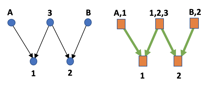
Return to the example of a random walker presented in the introduction, with an associated height unit structure illustrated in Fig. 2. Plugging into Eq. 37 and using obvious shorthand,
| (61) | ||||
| (62) |
Suppose that at the full system has a single specific state with probability . So . Suppose as well that the position in the lattice is uniformly random at . (For example, this will occur at large enough if the lattice has periodic boundary conditions and both and evolve by randomly choosing one of their two neighbors.) This means that knowing the values of at tells us nothing about the most recent values of not already given by the value of at , and so in particular tells us nothing about the most likely value of then. The same is true concerning the value of at . This all means that .
Combining gives . So Eq. 43 provides a strictly positive lower bound on the global EP. Note that this lower bound applies no matter what the dynamics of the process; it can be quasi-statically slow, it can involve Hamiltonian quenches, but so long as the unit structure does not change during the process, the EP is lower-bounded by . Furthermore, so long as the Hamiltonian is uniform at both and , the total work extracted in the process is the gain in entropy of the full system minus the global EP. Combining establishes that the total work extracted is upper-bounded by
| (63) |
Note that increasing while keeping constant means that the precise value tells us less about the precise lattice position. Eq. 63 tells us that increasing the significance of this way increases the upper bound on the total amount of work that can be extracted.
7 Discussion
In this paper I consider the thermodynamics of multi-dimensional systems evolving according to a continuous-time Markov chain. My main result is a strengthened version of the conventional second law, which applies whenever we have an a priori set of “dependency constraints” that for each coordinate specify which other coordinates can directly affect the dynamics of , via the rate matrix. The result holds for any coordinate system — the coordinates can be conventional phase space coordinates, they can be states of a set of separate interacting subsystems of an overall system, they can be positions in a sequence of more refined coarse-grainings of the state of the system, they can involve amounts of various chemicals in the system, etc.
To derive my result I first translate the dependency constraints into a “unit structure”. This gives a sigma algebra that groups the coordinates into overlapping sets, in a way that respects the dependency constraints. In general, any set of dependency constraints can be translated into more than one unit structure. In turn, any unit structure specifies an information-theoretic functional of distributions over the states of the system, called the “in-ex information”. To illustrate this, suppose the dependency constraints specify that each coordinate evolves autonomously, independent of the others. (As an example, this would be the case for the spatial coordinates of a particle freely evolving under over-damped Langevin dynamics in a uniform medium with no external forces.) We could then choose a unit structure that assigns each coordinate to its own unique unit. In this case the in-ex information reduces to the total correlation (sometimes called “multi-information”) of the system’s distribution, with each coordinate viewed as a separate random variable.
The strengthened version of the second law derived in this paper says that the entropy production (EP) of the system is lower-bounded by the difference between the beginning and ending values of the system’s in-ex information. This lower bound is independent of all features of the dynamics other than the the beginning distribution, the ending distribution, and the dependency constraints restricting how the dynamics could have caused the initial distribution to evolve into the ending distribution. Accordingly, we can use this strengthened second law to upper-bound the amount of work that can be extracted from a system as it evolves from one specified distribution to another [29, 14], in a way that accounts for dependency constraints governing the system’s dynamics. Similarly, this strengthened second law can be used to refine recent results in thermodynamics of feedback control [32], to account for dependency constraints in the system being controlled.
In contrast to other similar recently derived lower bounds on EP [46, 47], the one derived here does not require that the dynamics of the system be a multi-partite process. Nor does it require that local detailed balance holds. These two features mean the lower bound applies to any system undergoing continuous-time Markovian dynamics, even if the system has no natural thermodynamic interpretation. As a result, we can apply these results to everything from (Markov models of) evolving opinion networks to replicator dynamics of a population of evolving organisms.
A recent paper [20] used an information-geometric analysis to also derive bounds on minimal entropy production (EP) that arise due to constraints on the rate matrix of a system’s dynamics. To use the analysis in [20] one needs to first find an operator over the set of all joint distributions which both obeys the Pythagorean theorem of information theory and which commutes with the time-evolution operators defined by the set of allowed rate matrices. In general there are many such , but different ones will result in different bounds on EP.
The analog of in this paper is the set of dependency constraints.The analog to finding one (or more) ’s for the approach in this paper is choosing a coordinate system and associated unit structure that represents the dependency constraints and is rich enough for the lower bound on EP to be strictly positive. Similarly to the case with the approach in [20], where different all consistent with the constraints on the set of allowed rate matrices will result in different bounds on EP, in general different unit structures all consistent with the constraints on the set of allowed rate matrices will result in different bounds on EP.
[20] provides many examples of how constraints on the allowed rate matrices can be used to derive nonzero lower bounds on EP, including collective flashing ratchets, Szilard boxes where the particle is subject to a gravitational force in addition to driving by a piston, Szilard boxes where there are constraints on the way the piston can be used, evolving Ising spin systems, etc. Many of these examples can be formulated as systems evolving under dependency constraints (e.g., most of the examples involving in [20] “modularity constraints” can be directly formulated this way). Future work involves comparing the EP bounds in this paper to the ones in [20], and more generally trying to synthesize the two approaches.
I would like to thank Gülce Kardes, Artemy Kolchinsky and especially Farita Tasnim for feedback on drafts of this paper. This work was supported by the Santa Fe Institute, Grant No. CHE-1648973 from the US National Science Foundation and Grant No. FQXi-RFP-IPW-1912 from the FQXi foundation. The opinions expressed in this paper are those of the author and do not necessarily reflect the view of the National Science Foundation.
References
- [1] Andre C Barato and Udo Seifert, Stochastic thermodynamics with information reservoirs, Physical Review E 90 (2014), no. 4, 042150.
- [2] Stefano Bo, Marco Del Giudice, and Antonio Celani, Thermodynamic limits to information harvesting by sensory systems, Journal of Statistical Mechanics: Theory and Experiment 2015 (2015), no. 1, P01014.
- [3] Alexander B Boyd, Dibyendu Mandal, and James P Crutchfield, Thermodynamics of modularity: Structural costs beyond the landauer bound, Physical Review X 8 (2018), no. 3, 031036.
- [4] Rory A Brittain, Nick S Jones, and Thomas E Ouldridge, What we learn from the learning rate, Journal of Statistical Mechanics: Theory and Experiment 2017 (2017), no. 6, 063502.
- [5] Daniel M Busiello, Deepak Gupta, and Amos Maritan, Coarse-grained entropy production with multiple reservoirs: Unraveling the role of time scales and detailed balance in biology-inspired systems, Physical Review Research 2 (2020), no. 4, 043257.
- [6] Raphael Chetrite, ML Rosinberg, T Sagawa, and G Tarjus, Information thermodynamics for interacting stochastic systems without bipartite structure, Journal of Statistical Mechanics: Theory and Experiment 2019 (2019), no. 11, 114002.
- [7] Thomas M. Cover and Joy A. Thomas, Elements of information theory, John Wiley & Sons, 2012.
- [8] Gianmaria Falasco and Massimiliano Esposito, Dissipation-time uncertainty relation, Physical Review Letters 125 (2020), no. 12, 120604.
- [9] Gianmaria Falasco, Massimiliano Esposito, and Jean-Charles Delvenne, Unifying thermodynamic uncertainty relations, New Journal of Physics 22 (2020), no. 5, 053046.
- [10] Todd R Gingrich and Jordan M Horowitz, Fundamental bounds on first passage time fluctuations for currents, Physical Review Letters 119 (2017), no. 17, 170601.
- [11] Deepak Gupta and Daniel M Busiello, Thermodynamic bound on speed limit in systems with unidirectional transitions and a tighter bound, arXiv preprint arXiv:2009.11115 (2020).
- [12] D. Hartich, A. C. Barato, and U. Seifert, Stochastic thermodynamics of bipartite systems: transfer entropy inequalities and a Maxwell’s demon interpretation, Journal of Statistical Mechanics: Theory and Experiment 2014 (2014), no. 2, P02016.
- [13] David Hartich, Andre C. Barato, and Udo Seifert, Sensory capacity: an information theoretical measure of the performance of a sensor, Physical Review E 93 (2016), no. 2, arXiv: 1509.02111.
- [14] H-H Hasegawa, J Ishikawa, K Takara, and DJ Driebe, Generalization of the second law for a nonequilibrium initial state, Physics Letters A 374 (2010), no. 8, 1001–1004.
- [15] J.M. Horowitz and T.R. Gingrich, Thermodynamic uncertainty relations constrain non-equilibrium fluctuations, Nature Physics (2019).
- [16] Jordan M. Horowitz, Multipartite information flow for multiple Maxwell demons, Journal of Statistical Mechanics: Theory and Experiment 2015 (2015), no. 3, P03006.
- [17] Jordan M Horowitz and Massimiliano Esposito, Thermodynamics with continuous information flow, Physical Review X 4 (2014), no. 3, 031015.
- [18] Jordan M. Horowitz and Todd R. Gingrich, Proof of the finite-time thermodynamic uncertainty relation for steady-state currents, Phys. Rev. E 96 (2017), 020103.
- [19] Christopher Jarzynski, Hamiltonian derivation of a detailed fluctuation theorem, Journal of Statistical Physics 98 (2000), no. 1-2, 77–102.
- [20] Artemy Kolchinsky and David H Wolpert, Entropy production and thermodynamics of information under protocol constraints, arXiv:2008.10764, 2020.
- [21] Timur Koyuk and Udo Seifert, Thermodynamic uncertainty relation for time-dependent driving, Physical Review Letters 125 (2020), no. 26, 260604.
- [22] Adam Lipowski, António Luis Ferreira, Dorota Lipowska, and Krzysztof Gontarek, Phase transitions in ising models on directed networks, Physical Review E 92 (2015), no. 5, 052811.
- [23] Kangqiao Liu, Zongping Gong, and Masahito Ueda, Thermodynamic uncertainty relation for arbitrary initial states, Physical Review Letters 125 (2020), no. 14, 140602.
- [24] Sarah AM Loos and Sabine HL Klapp, Irreversibility, heat and information flows induced by non-reciprocal interactions, New Journal of Physics 22 (2020), no. 12, 123051.
- [25] William McGill, Multivariate information transmission, Transactions of the IRE Professional Group on Information Theory 4 (1954), no. 4, 93–111.
- [26] Izaak Neri, Dissipation bounds the moments of first-passage times of dissipative currents in nonequilibrium stationary states, arXiv preprint arXiv:2103.15007 (2021).
- [27] Izaak Neri, Édgar Roldán, and Frank Jülicher, Statistics of infima and stopping times of entropy production and applications to active molecular processes, Physical Review X 7 (2017), no. 1, 011019.
- [28] Manaka Okuyama and Masayuki Ohzeki, Quantum speed limit is not quantum, Physical Review Letters 120 (2018), no. 7, 070402.
- [29] Juan MR Parrondo, Jordan M Horowitz, and Takahiro Sagawa, Thermodynamics of information, Nature Physics 11 (2015), no. 2, 131–139.
- [30] Édgar Roldán, Izaak Neri, Meik Dörpinghaus, Heinrich Meyr, and Frank Jülicher, Decision making in the arrow of time, Physical review letters 115 (2015), no. 25, 250602.
- [31] Takahiro Sagawa and Masahito Ueda, Minimal energy cost for thermodynamic information processing: measurement and information erasure, Physical Review Letters 102 (2009), no. 25, 250602.
- [32] , Generalized jarzynski equality under nonequilibrium feedback control, Physical Review Letters 104 (2010), no. 9, 090602.
- [33] , Nonequilibrium thermodynamics of feedback control, Physical Review E 85 (2012), no. 2, 021104.
- [34] Alejandro D Sánchez, Juan M López, and Miguel A Rodriguez, Nonequilibrium phase transitions in directed small-world networks, Physical review letters 88 (2002), no. 4, 048701.
- [35] Udo Seifert, Stochastic thermodynamics, fluctuation theorems and molecular machines, Reports on Progress in Physics 75 (2012), no. 12, 126001.
- [36] Naoto Shiraishi, Ken Funo, and Keiji Saito, Speed limit for classical stochastic processes, Physical Review Letters 121 (2018), no. 7.
- [37] Naoto Shiraishi and Takahiro Sagawa, Fluctuation theorem for partially masked nonequilibrium dynamics, Physical Review E 91 (2015), no. 1, 012130.
- [38] Richard P Stanley, Enumerative combinatorics volume 1 second edition, Cambridge studies in advanced mathematics (2011).
- [39] Philipp Strasberg and Massimiliano Esposito, Stochastic thermodynamics in the strong coupling regime: An unambiguous approach based on coarse graining, Physical Review E 95 (2017), no. 6, 062101.
- [40] Farita Tasnim and David H Wolpert, Thermodynamic speed limits for multiple, co-evolving systems, arXiv preprint arXiv:2107.12471 (2021).
- [41] Hu Kuo Ting, On the amount of information, Theory of Probability & Its Applications 7 (1962), no. 4, 439–447.
- [42] Christian Van den Broeck and Massimiliano Esposito, Ensemble and trajectory thermodynamics: A brief introduction, Physica A: Statistical Mechanics and its Applications 418 (2015), 6–16.
- [43] Tan Van Vu, Yoshihiko Hasegawa, et al., Unified approach to classical speed limit and thermodynamic uncertainty relation, Physical Review E 102 (2020), no. 6, 062132.
- [44] Gatien Verley, Christian Van den Broeck, and Massimiliano Esposito, Work statistics in stochastically driven systems, New Journal of Physics 16 (2014), no. 9, 095001.
- [45] David H. Wolpert, The stochastic thermodynamics of computation, Journal of Physics A: Mathematical and Theoretical (2019).
- [46] David H Wolpert, Fluctuation theorems for multipartite processes, arXiv:2003.11144:v5 (2020).
- [47] , Minimal entropy production rate of interacting systems, New Journal of Physics 22 (2020), no. 11, 113013.
- [48] David H. Wolpert, Uncertainty relations and fluctuation theorems for Bayes nets, Phys. Rev. Lett. 125 (2020), 200602.
- [49] David H. Wolpert, Combining lower bounds on entropy production in complex systems with multiple interacting components, Encyclopedia of Entropy Across the Disciplines (Z. Nashed W. Freeden, ed.), World Scientific Publishing Co., Inc., 2022.
- [50] Yunxin Zhang, Comment on" speed limit for classical stochastic processes", arXiv e-prints (2018), arXiv–1811.
Supplementary material for Strengthened second law for multi-dimensional systems coupled to multiple thermodynamic reservoirs
David H. Wolpert1
1Santa Fe Institute, New Mexico, USA
Complexity Science Hub, Vienna
Arizona State University, Tempe, Arizona
International Center for Theoretical Physics, Italy
http://davidwolpert.weebly.com
Appendix A Proof that the intersections of two units is a unit
Without loss of generality, suppose that there are exactly three coordinates, with their values written as , respectively, and hypothesize that the joint state evolves as a unit, as does . We need to prove that also evolves on its own as a unit.
Let be the overall rate matrix of the system at (implicit) time . By our two hypotheses, there are two rate matrices , such that
| (A64) | ||||
| (A65) |
Since these equations must hold for all , by considering delta function ’s we see that
| (A66) | ||||
| (A67) |
Next, define
| (A68) |
Summing both sides of Eq. D88 over and then plugging in Eq. A67,
| (A69) | ||||
| (A70) |
Since the RHS is independent of , so must the LHS be. So must be independent of . Moreover, combining Eqs. A68 and A67 shows that for all . Therefore is a properly normalized rate matrix.
To complete the proof, expand
| (A71) | ||||
| (A72) | ||||
| (A73) | ||||
| (A74) | ||||
| (A75) |
Appendix B Illustration of Eq. 9
Suppose that each coordinate of has the same dimension, . Choose any subset of the coordinates, , coordinate and any stochastic matrix . Then
| (B76) |
is a properly normalized rate matrix over all of , since for all , .
In addition, choose , and choose
| (B77) |
Then obeys Eq. 9 in the main text, since for all ,
| (B78) | ||||
| (B79) |
So is a unit.
Appendix C Proof of Eq. 21
Expand
| (C80) | ||||
| (C81) | ||||
| (C82) | ||||
| (C83) | ||||
| (C84) | ||||
| (C85) |
where for convenience I have switched back and forth between the shorthand of Eq. 14.
Appendix D Proof of Eq. 34
First, note that by Eq. 9, for all conditional distributions , for all ,
| (D86) | ||||
| (D87) |
where the second equality follows from Appendix M. Next, use Eq. 32 to expand
| (D88) |
In addition, using the log sum inequality [7] shows that for each , the associated value of the first term in the inner sum on the RHS of Eq. D88 is bounded by
| (D89) |
where the second line uses Eq. D87.
Combining and using Eq. D87 again establishes that
| (D90) |
Again plugging into Eq. 3.13, this time for the EP rate of unit , completes the proof.
Appendix E Proof of Eq. 38
We are given some composite system with unit structure . Fix the time and make it implicit for the rest of this appendix. Define as the set of all state transitions in , involving an arbitrary number of the coordinates in . (So there are elements of , where is the number of joint states of the multi-dimensional system.)
For any unit define as the set of all state transitions such that both and . (Intuitively, is the set of all state transitions that do not modify any of the coordinates outside of and that are allowed under the CTMC.) Note that if . So is a locally finite poset, ordered by the set inclusion relation.
Due to our assumption that the unit structure is flush, no state transition can occur that has the property of simultaneously changing the state of all coordinates in an arbitrary set unless is a subset of a unit (i.e., there is no pair that has that property where both and ). This means that every element of allowed by the CTMC is contained in at least one element of . So is a cover of the set of all state transitions allowed by the CTMC.
Next, due to our assumption that there are no two equivalent units in the unit structure, the set of all transitions in a set uniquely specifies , i.e., there is a bijection between and . Due to this, without any ambiguity we can define a function by setting
| (E91) | ||||
| (E92) | ||||
| (E93) |
for all , and similarly setting . (Note that if , then this second definition is redundant.)
In addition, unit structures are closed under intersection. As described in the text, this means that generates a sigma algebra over coordinates, and we can use the function to generate a signed measure over that sigma algebra. In the same way, generates a sigma algebra over state transitions, and the function generates a signed measure of that sigma algebra. We can apply all the steps in the usual derivation of the inclusion-exclusion principle for signed measures from Rota’s theorem [38] to that signed measure generated by . This allow us to write
| (E94) |
Plugging in the definition of completes the proof.
Appendix F Discussion of Eq. 3.21 for the case of parallel bit erasure
Suppose our system comprises two physically separated subsystems where that state space of both subsystems are a bit. Suppose as well that subsystem gets erased in the process, and the initial distribution is uniform random between the joint state where both bits equal , and the joint state where both bits equal , with no other possibilities. If the dynamics is a single unit, so that the rate matrix of subsystem can depend on the (unchanging) state of subsystem , EP can equal . If instead there are two separate units, so that the rate matrix of subsystem cannot depend on the state of subsystem , minimal EP is instead .
To understand this, suppose that there is a (time-varying) Hamiltonian and that the full system’s (time-varying) rate matrix always obeys LDB for that Hamiltonian. So to have the global EP during the full process equal zero, there would have to be a trajectory of such Hamiltonians such that at all times the system was always at equilibrium for the associated Hamiltonian. Furthermore, because we’re assuming the system is governed by a CTMC, the distribution can never change discontinuously during times within the process, and therefore neither can the Hamiltonian.
Given this, suppose that there is no continuous trajectory of such distributions that is always a product distribution and has the desired initial and final forms, . (For example, this is the case if the two subsystems are statistically coupled at .) Then by the always-at-equilibrium condition for zero EP, there must be a time at which the Hamiltonian cannot be written as a sum of a function of plus a function of , but instead must nonlinear couple them. By our assumption of LDB, this would then mean that at that time , the full rate matrix of the joint system must couple those two subsystems, which in turn means that the rate matrix of one of the two subsystems must depend on the state of the other subsystem 1212 12 Note that how much EP in a process is generated is independent of whether the system obeys LDB, or even whether there is a Hamiltonian. On the other hand, if there is a Hamiltonian that obeys LDB, we know that zero EP would be generated iff the system were always at equilibrium.
To apply this to our two-subsystem example, simply note that the beginning distribution is not a product distribution. Therefore the condition for zero EP is violated if neither of the rate matrices of the two subsystems depends on the other subsystem’s state.
Appendix G Proofs related to Eq. 4.1
To begin, I need to define , a set of distributions over the Boolean hypercube, . After that, I define a “centering distribution” to be any convex combination of the elements of which equals , the uniform distribution over the Boolean hypercube. My first main result, presented in Proposition G.1, is a function taking each such centering distribution to a different lower bound on global EP.
The set is the union of two sets of distributions over , which I define in succession:
I) For any , write for the distribution over which is all ’s except for a in its component. Using this notation, define as the set of all distributions over which obey at least one of the following three conditions:
- 1.
for some whose height ;
- 2.
for some ;
- 3.
for a ;
I will refer to any distributions that obey these conditions as type-, type-, and type- distributions, respectively.
To provide examples, consider the dependency graph illustrated in the right panel in Fig. 3. There are four associated type-1 distributions, , i.e., delta functions over the units , respectively. There are six type- distributions; for example, the (unique) one for unit is .
Next, note that units are all units contained in unit (i.e., those nodes are contained in the family of node ). Similarly, are both units contained in . Therefore the units that are in but not in are . Accordingly, the (unique) type- distribution for the pair of units is .

II) For any unit , write for any set of coordinates which can be represented by a unit structure 1313 13 There is always at least one such for any non-leaf , given by the set of coordinates . Note that in general, any such set of coordinates can be represented by more than one unit . For example, suppose there are leaves in that have only one parent, i.e., there are units in that are only proper subsets of one other unit in . Then there is both a unit structure that contains those leaves that represents , and a unit structure that does not contain those leaves but still represents .. Define as the set of all distributions over of the form
| (G95) |
for some and associated unit . I will refer to any such distribution as a type- distribution. Note that any type-4 distribution uniquely specifies both and . Given this, I will sometimes abuse notation and write for the unit structure with the single unit specified by a type-4 distribution .
To illustrate type- distributions, again consider Fig. 3. Choose . So . Choose to be the set of coordinates with the associated unit . So . The associated type- distribution is .
As shorthand, write . As a final piece of terminology, let be any set of distributions over some shared space. I will say that is centered if there exists a centering distribution such that equals the uniform distribution. Note that the set of all centering distributions of any is a convex polytope.
The following result involving centering distributions is proven in Appendix H:
Proposition G.1.
If is a centering distribution for , then
Note that the values of the in-ex informations and at the beginning and end of the process are fully specified by and . So given a centering distribution, Proposition G.1 provides a lower bound on global EP defined purely in terms of and . The precise rate matrix is irrelevant, so long as it has as a unit structure and maps to . Note as well that the sum in Proposition G.1 only extends over distributions in . The role of the distributions in is indirect; in general they are necessary to construct a centering distribution , and thereby constrain the possible values of for the distributions in .
As an example of Proposition G.1, first recall that even though each unit evolves autonomously, in general we cannot choose all the rate matrices so that every . In particular, if has a non-trivial unit structure within it, then Eq. 3.21 will apply for the choice , potentially providing a strictly positive lower bound to . As a result, in general we cannot choose all the rate matrices so that , and so cannot in general lower bound by .
On the other hand, suppose that has height . (So there are no units such that .) Then all delta function distributions over are type-1 distributions, and so contained in . Accordingly, the unit structure is centered by a distribution that is uniform over all and equals for all . Plugging this into Proposition G.1 establishes that the EP of any process with a height-2 unit structure is in fact lower-bounded by . This provides the formal justification for Eq. 4.1.
Moreover, in general, we can represent any process by using a unit structure of height . (For example, we can do that by combining all coordinates that are members of some unit that is not a root node of , into one, overarching unit.) Accordingly, for any process, we can always find an associated unit structure for which .
In addition, it is proven in Appendix I that for any unit structure , no matter what its height, is centered. (The set of all associated centering distributions of is the convex polytope discussed in the introduction.) In general, finding the optimal such centering distribution — the one that maximizes the bound in Proposition G.1, and so provides the strongest lower bound on global EP — only requires solving a linear programming problem.
Unfortunately, there are some unit structures where the bound in Proposition G.1 is negative for an appropriate initial distribution and conditional distribution consistent with , no matter what centering distribution we use. In such cases, Proposition G.1 does not provide a stronger bound on EP than the conventional second law.
On the other hand, as illustrated in the main text, often the bound in Proposition G.1 will be stronger than the conventional second law. Indeed, for every unit structure , and every associated centering distribution, there are initial distributions and conditional distributions that are consistent with where the EP bound in Proposition G.1 is at least as strong as the second law:
Proposition G.2.
Let be any unit structure that does not have itself as a member. Then there exists an initial joint distribution and a conditional distribution consistent with such that for any associated centering distribution ,
| (G96) |
for every rate matrix that both implements that and obeys the unit structure.
(See Appendix J for proof.)
In addition, even if , often we can use Eq. 3.21 directly to provide a non-negative lower bound on the global EP, by constructing a lower bound on which is bigger than . To construct such a bound, first note that since there is no unit structure within leaf units of the dependency graph, in theory we can implement all such units with zero local EP. Next, for any unit that is a parent of a leaf unit, we can often use Eq. 15 in [47] (or its corollary, Eq. 17) to construct strictly positive lower bounds on .
Write the polytope of all centering distributions of the unit structure as , and write the strongest lower bound on EP given by Proposition G.1 as
| (G97) |
Combining Propositions G.1 and G.2 establishes that for any unit structure there are pairs of and a conditional distribution consistent with such that
| (G98) | ||||
| (G99) |
In contrast, the conventional second law says only that , no matter what , or are.
Summarizing, suppose we are given a unit structure that applies to the rate matrix at all times, an initial distribution , and a conditional distribution consistent with . Then we know that is a lower bound on the EP, for any that is a centering distribution for . These lower bounds are simple to evaluate, and are often stronger than the second law. We can find the strongest such lower bound on EP due to the unit structure by solving a linear programming problem.
Furthermore, in general, it is possible to represent any given set of constraints with more than one unit structure. Each one of them results in its own strongest lower bound on EP, given by solving the associated linear programming problem. So to find the strongest version of the second law for a given set of constraints, we should solve all the linear programming problems specified by the unit structures that can represent those constraints.
This result extends the previous strengthenings of the second law derived in [45, 20, 3], which all assume that the units have no overlap, to the case where the units may overlap with one another in arbitrary ways, even if none of the coordinates are fixed in the dynamics. In addition to this result, which maps an arbitrary set of constraints, a and a to a lower bound on EP, a second result is that for any set of constraints, there is a and that results in a strictly positive lower bound on EP, stronger than the conventional second law.
Appendix H Proof of Proposition G.1
The proof has two parts. First, I construct a function such that for all units , . (Note that in general, any coordinate will be in more than one unit , and so this function is the solution to a set of coupled equations.) I will then apply the inclusion-exclusion principle with this in order to replace the first in-ex sums over unit on the RHS of Eq. 3.21 with a conventional sum over coordinates, .
In the second part of the proof I use the hypothesized existence of a centering distribution to provide a lower bound on , expressed purely in terms of and . Plugging in to Eq. 3.21 then completes the proof.
To begin, for each unit , define as the set of all coordinates in that are not in any of the units in . (As an example, in Fig. 1 in the main text, is the pair of coordinates and .) Because is closed under intersections and covers , every coordinate is in for exactly one unit . Moreover, because there are no vacuous units allowed, is nonempty for every unit . Note that if for two units , then the coordinates in must evolve independently of the states of any coordinates in , but the reverse need not be true. In other words, if there is an edge from to , then there may be coordinates in whose dynamics depends on the state of coordinates in , but not vice-versa.
For all , let be the set of all nodes in , with height . So in particular, is the the set all units with no subunits. For every , for all coordinates , set
| (H100) |
So by construction, for all ,
| (H101) |
Since for all , this means that for all .
Next, note that any for any , the set of units in is closed under intersections. This allows us to define
| (H102) |
for all , all , and all . (Note that any such will be assigned a value exactly once in this procedure.)
In general, it could be that is negative. Note though that since no two units in have any overlap, for all ,
| (H103) | ||||
| (H104) |
Therefore by Eq. H102, for all ,
| (H105) | ||||
| (H106) | ||||
| (H107) |
i.e., Eq. H101 holds for unit .
Next, assume that Eq. H101 holds for all for some integer . Then by Eq. H102 and the inclusion-exclusion principle, for any ,
| (H108) | ||||
| (H109) | ||||
| (H110) | ||||
| (H111) |
(Note that the inclusion-exclusion principle holds for arbitrary functions , not just for nowhere-negative functions.) Since , this means that we are guaranteed that .
Iterate this procedure going from nodes in to those in until all units have been considered, so that values have been assigned to all coordinates . By induction, at the end of this procedure, for all units , Eq. H101 will hold and . In addition, by the inclusion-exclusion principle,
| (H112) | ||||
| (H113) |
(Note that since , Eq. H111 does not imply that . So we cannot combine Eq. H113 with the fact that global EP is to establish that is also non-negative.)
It will be convenient to define new variables that equal sums of over small sets of coordinates . For all , define
| (H114) | ||||
| (H115) |
where the second line follows from Eq. H102. Since each coordinate is in for exactly one unit , for any ,
| (H116) | ||||
| (H117) | ||||
| (H118) |
where the last line uses Eq. H111. Using similar reasoning shows that . Combining this with Eq. H113 and Eq. 40 gives
| (H119) |
This completes the first part of the proof. In the second part I derive a lower bound on the RHS of Eq. H119. First, to reduce the complexity of the equations, I will translate all distributions into binary-valued vectors:
- 1.
for any type-1 distribution ;
- 2.
for any type-2 distribution ;
- 3.
for any type-3 distribution ;
- 4.
for any type-4 distribution ;
Note that every component of every vector is either a or a . I will refer to any vectors that obey condition (1) as type- vectors, and similarly for vectors obeying conditions (2), (3) and / or (4).
Now make three suppositions. First, suppose that for all vectors of types or ,
| (H120) |
Next, suppose that for all vectors of type-, and all associated unit structures ,
| (H121) |
Now, hypothesize that there is a centering vector all of whose components are non-negative such that
| (H122) |
for all . Multiplying both sides of Eq. H122 by , summing over , and then plugging in Eqs. H120 and H121, we see that if those three equations hold,
| (H123) |
Plugging this into Eq. H119 shows that if we can prove that the suppositions Eqs. H120 and H121 always hold, then we will have proven that for any centering vector ,
| (H124) |
To begin, use Eq. H115 to conclude that for all (which have no descendants) and so for all . Next, combine this fact that for all leaf nodes with Eqs. 35 and H118 to also conclude that for all . Combining these two results means that Eq. H120 holds for all type-1 vectors .
Next, note that Eq. H118 means that for any ,
| (H125) |
So by the non-negativity of local EP, for all ,
| (H126) |
This means that Eq. H120 holds for all type-2 vectors .
Now consider any pair of nodes . Using Eq. H118 for both and and then applying Eq. 3.15 establishes that
| (H127) | ||||
| (H128) |
This means that Eq. H120 also holds for all type-3 vectors . Combining establishes our first goal, of showing that Eq. H120 holds for all vectors , of types or .
Next, consider any pair of a unit and set of coordinates such that there is a unit structure . Use Eq. H111, the inclusion-exclusion principle, Eq. H114, and then Eq. H118 to expand
| (H129) | ||||
| (H130) | ||||
| (H131) | ||||
| (H132) | ||||
| (H133) | ||||
| (H134) | ||||
| (H135) |
Eq. 3.22 then establishes that
| (H136) |
Plugging this into the definition of type- vectors for and confirms that Eq. H120 holds.
Combining establishes that for any centering vector ,
| (H137) |
Finally, normalize each vector to recover the distributions , and define the distribution by normalizing . It follows that is the uniform distribution, so that is a centering distribution. In addition, Eq. H137 gets converted into the bound in Proposition G.1. This completes the proof of Proposition G.1.
Appendix I Proof that any unit structure is centered
To begin, choose to be the set of all type-1 distributions, i.e., is the set of all distributions for any of height .
Next, for each of height greater than , plug and any arbitrary single one of the possible unit structures into Eq. H122 to define a distribution
| (I138) | ||||
| (I139) |
and associated unit structure . Choose to be the set of all such , one per , as one ranges over all of height greater than .
By construction, is exactly the set of all vectors as one ranges over all . Accordingly, the sum of all distributions in is , and the average of those distributions is the uniform distribution, . Therefore the set of those vectors is centered, where the centering distribution for all . This completes the proof.
Appendix J Proof of Proposition G.2
First, note that for a uniform distribution over the states of the multi-dimensional system, the entropy of every coordinate with states is . Furthermore, no matter what the unit structure is, one can create a process consistent with that structure that results in this uniform distribution as the final distribution. (Just choose the rate matrix so that by the end of the process, for each coordinate , has been uniformly randomized.)
Now assign values to all coordinates. By construction, for all units , . In addition,
| (J140) |
by the inclusion-exclusion principle. But the sum on the RHS just equals , the entropy of the full system, since the coordinates are statistically independent under the final distribution. Therefore for this ending distribution. Similarly, for this ending distribution, for every .
So to find a situation where Proposition G.1 holds, it suffices to find an initial distribution such that while for all . To do that, label the states of each coordinate by the first counting numbers. Define , and define as the (units corresponding to the) root nodes of the dependency graph . Note that since by hypothesis , there must be at least two distinct root nodes in . Furthermore, since there are no vacuous units in a composite system, all of (the units corresponding to) those root nodes contain coordinates that are not in any other units, i.e., for all , .
Next, define , and fix the state of each coordinate , i.e., set the distribution over the state of that coordinate to a delta function. Set the joint distribution over the remaining coordinates to
| (J141) |
So all coordinates that only occur in a single root unit are perfectly coupled with one another, with a uniform distribution over the set of possible joint states they can adopt.
The entropy of the full joint distribution defined this way is . So to prove that we need to show that
| (J142) |
To do that, assign the value to all coordinates . For each coordinate , where is the unique unit containing , assign the value
| (J143) |
where is the number of elements in .
By construction, for all units ,
| (J144) |
Accordingly, by the inclusion-exclusion principle
| (J145) | ||||
| (J146) |
Since contains at least two units, this means that
| (J147) |
In addition, the entropy of every unit equals . Accordingly, for all .
This completes the proof.
Appendix K Proofs of results for thermodynamics of feedback control of composite unit structures
The growth of the entropy of unit during the process changes when we expand it into the unit that includes . To calculate how much it changes, first, since does not change state during the process, the entropy of each unit grows during the process by the change in conditional entropy,
| (K148) |
where are given by Eq. 5.1, 5.2, respectively. In contrast, the growth of entropy in the unit in the original, no-feedback process is
| (K149) |
This just equals , due to our assumption that the initial and final marginal distributions over are the same regardless of whether there is a feedback apparatus.
Combining, we see that the change in the growth of entropy of unit when we add the feedback apparatus is the drop of mutual information,
| (K150) |
This is true for every unit , and for itself. Plugging this fact into Eq. 4.1 gives Eq. 5.4.
Next, reuse the reasoning behind Eq. K148 to establish that the lower bound on EP in the feedback scenario is
| (K151) |
In addition, the maximal work that can be extracted from the system under feedback control without consideration of the unit structure of the system is [31, 29, 20]
| (K152) |
(under the common assumption that the Hamiltonian at both and is uniform, and in units of ). Subtracting the lower EP bound, Eq. K151, from Eq. K152 establishes Eq. 5.5.
Appendix L Proof of Proposition 2.1
By Eq. 10,
| (L153) | ||||
| (L154) | ||||
| (L155) | ||||
| (L156) | ||||
| (L157) |
where the penultimate line sums the Kronecker delta function over all , and the last line uses the fact that for all such that , the inner sum over equals zero, by normalization.
Appendix M Proof of Proposition 2.2
References
- [1] Andre C Barato and Udo Seifert, Stochastic thermodynamics with information reservoirs, Physical Review E 90 (2014), no. 4, 042150.
- [2] Stefano Bo, Marco Del Giudice, and Antonio Celani, Thermodynamic limits to information harvesting by sensory systems, Journal of Statistical Mechanics: Theory and Experiment 2015 (2015), no. 1, P01014.
- [3] Alexander B Boyd, Dibyendu Mandal, and James P Crutchfield, Thermodynamics of modularity: Structural costs beyond the landauer bound, Physical Review X 8 (2018), no. 3, 031036.
- [4] Rory A Brittain, Nick S Jones, and Thomas E Ouldridge, What we learn from the learning rate, Journal of Statistical Mechanics: Theory and Experiment 2017 (2017), no. 6, 063502.
- [5] Daniel M Busiello, Deepak Gupta, and Amos Maritan, Coarse-grained entropy production with multiple reservoirs: Unraveling the role of time scales and detailed balance in biology-inspired systems, Physical Review Research 2 (2020), no. 4, 043257.
- [6] Raphael Chetrite, ML Rosinberg, T Sagawa, and G Tarjus, Information thermodynamics for interacting stochastic systems without bipartite structure, Journal of Statistical Mechanics: Theory and Experiment 2019 (2019), no. 11, 114002.
- [7] Thomas M. Cover and Joy A. Thomas, Elements of information theory, John Wiley & Sons, 2012.
- [8] Gianmaria Falasco and Massimiliano Esposito, Dissipation-time uncertainty relation, Physical Review Letters 125 (2020), no. 12, 120604.
- [9] Gianmaria Falasco, Massimiliano Esposito, and Jean-Charles Delvenne, Unifying thermodynamic uncertainty relations, New Journal of Physics 22 (2020), no. 5, 053046.
- [10] Todd R Gingrich and Jordan M Horowitz, Fundamental bounds on first passage time fluctuations for currents, Physical Review Letters 119 (2017), no. 17, 170601.
- [11] Deepak Gupta and Daniel M Busiello, Thermodynamic bound on speed limit in systems with unidirectional transitions and a tighter bound, arXiv preprint arXiv:2009.11115 (2020).
- [12] D. Hartich, A. C. Barato, and U. Seifert, Stochastic thermodynamics of bipartite systems: transfer entropy inequalities and a Maxwell’s demon interpretation, Journal of Statistical Mechanics: Theory and Experiment 2014 (2014), no. 2, P02016.
- [13] David Hartich, Andre C. Barato, and Udo Seifert, Sensory capacity: an information theoretical measure of the performance of a sensor, Physical Review E 93 (2016), no. 2, arXiv: 1509.02111.
- [14] H-H Hasegawa, J Ishikawa, K Takara, and DJ Driebe, Generalization of the second law for a nonequilibrium initial state, Physics Letters A 374 (2010), no. 8, 1001–1004.
- [15] J.M. Horowitz and T.R. Gingrich, Thermodynamic uncertainty relations constrain non-equilibrium fluctuations, Nature Physics (2019).
- [16] Jordan M. Horowitz, Multipartite information flow for multiple Maxwell demons, Journal of Statistical Mechanics: Theory and Experiment 2015 (2015), no. 3, P03006.
- [17] Jordan M Horowitz and Massimiliano Esposito, Thermodynamics with continuous information flow, Physical Review X 4 (2014), no. 3, 031015.
- [18] Jordan M. Horowitz and Todd R. Gingrich, Proof of the finite-time thermodynamic uncertainty relation for steady-state currents, Phys. Rev. E 96 (2017), 020103.
- [19] Christopher Jarzynski, Hamiltonian derivation of a detailed fluctuation theorem, Journal of Statistical Physics 98 (2000), no. 1-2, 77–102.
- [20] Artemy Kolchinsky and David H Wolpert, Entropy production and thermodynamics of information under protocol constraints, arXiv:2008.10764, 2020.
- [21] Timur Koyuk and Udo Seifert, Thermodynamic uncertainty relation for time-dependent driving, Physical Review Letters 125 (2020), no. 26, 260604.
- [22] Adam Lipowski, António Luis Ferreira, Dorota Lipowska, and Krzysztof Gontarek, Phase transitions in ising models on directed networks, Physical Review E 92 (2015), no. 5, 052811.
- [23] Kangqiao Liu, Zongping Gong, and Masahito Ueda, Thermodynamic uncertainty relation for arbitrary initial states, Physical Review Letters 125 (2020), no. 14, 140602.
- [24] Sarah AM Loos and Sabine HL Klapp, Irreversibility, heat and information flows induced by non-reciprocal interactions, New Journal of Physics 22 (2020), no. 12, 123051.
- [25] William McGill, Multivariate information transmission, Transactions of the IRE Professional Group on Information Theory 4 (1954), no. 4, 93–111.
- [26] Izaak Neri, Dissipation bounds the moments of first-passage times of dissipative currents in nonequilibrium stationary states, arXiv preprint arXiv:2103.15007 (2021).
- [27] Izaak Neri, Édgar Roldán, and Frank Jülicher, Statistics of infima and stopping times of entropy production and applications to active molecular processes, Physical Review X 7 (2017), no. 1, 011019.
- [28] Manaka Okuyama and Masayuki Ohzeki, Quantum speed limit is not quantum, Physical Review Letters 120 (2018), no. 7, 070402.
- [29] Juan MR Parrondo, Jordan M Horowitz, and Takahiro Sagawa, Thermodynamics of information, Nature Physics 11 (2015), no. 2, 131–139.
- [30] Édgar Roldán, Izaak Neri, Meik Dörpinghaus, Heinrich Meyr, and Frank Jülicher, Decision making in the arrow of time, Physical review letters 115 (2015), no. 25, 250602.
- [31] Takahiro Sagawa and Masahito Ueda, Minimal energy cost for thermodynamic information processing: measurement and information erasure, Physical Review Letters 102 (2009), no. 25, 250602.
- [32] , Generalized jarzynski equality under nonequilibrium feedback control, Physical Review Letters 104 (2010), no. 9, 090602.
- [33] , Nonequilibrium thermodynamics of feedback control, Physical Review E 85 (2012), no. 2, 021104.
- [34] Alejandro D Sánchez, Juan M López, and Miguel A Rodriguez, Nonequilibrium phase transitions in directed small-world networks, Physical review letters 88 (2002), no. 4, 048701.
- [35] Udo Seifert, Stochastic thermodynamics, fluctuation theorems and molecular machines, Reports on Progress in Physics 75 (2012), no. 12, 126001.
- [36] Naoto Shiraishi, Ken Funo, and Keiji Saito, Speed limit for classical stochastic processes, Physical Review Letters 121 (2018), no. 7.
- [37] Naoto Shiraishi and Takahiro Sagawa, Fluctuation theorem for partially masked nonequilibrium dynamics, Physical Review E 91 (2015), no. 1, 012130.
- [38] Richard P Stanley, Enumerative combinatorics volume 1 second edition, Cambridge studies in advanced mathematics (2011).
- [39] Philipp Strasberg and Massimiliano Esposito, Stochastic thermodynamics in the strong coupling regime: An unambiguous approach based on coarse graining, Physical Review E 95 (2017), no. 6, 062101.
- [40] Farita Tasnim and David H Wolpert, Thermodynamic speed limits for multiple, co-evolving systems, arXiv preprint arXiv:2107.12471 (2021).
- [41] Hu Kuo Ting, On the amount of information, Theory of Probability & Its Applications 7 (1962), no. 4, 439–447.
- [42] Christian Van den Broeck and Massimiliano Esposito, Ensemble and trajectory thermodynamics: A brief introduction, Physica A: Statistical Mechanics and its Applications 418 (2015), 6–16.
- [43] Tan Van Vu, Yoshihiko Hasegawa, et al., Unified approach to classical speed limit and thermodynamic uncertainty relation, Physical Review E 102 (2020), no. 6, 062132.
- [44] Gatien Verley, Christian Van den Broeck, and Massimiliano Esposito, Work statistics in stochastically driven systems, New Journal of Physics 16 (2014), no. 9, 095001.
- [45] David H. Wolpert, The stochastic thermodynamics of computation, Journal of Physics A: Mathematical and Theoretical (2019).
- [46] David H Wolpert, Fluctuation theorems for multipartite processes, arXiv:2003.11144:v5 (2020).
- [47] , Minimal entropy production rate of interacting systems, New Journal of Physics 22 (2020), no. 11, 113013.
- [48] David H. Wolpert, Uncertainty relations and fluctuation theorems for Bayes nets, Phys. Rev. Lett. 125 (2020), 200602.
- [49] David H. Wolpert, Combining lower bounds on entropy production in complex systems with multiple interacting components, Encyclopedia of Entropy Across the Disciplines (Z. Nashed W. Freeden, ed.), World Scientific Publishing Co., Inc., 2022.
- [50] Yunxin Zhang, Comment on" speed limit for classical stochastic processes", arXiv e-prints (2018), arXiv–1811.