Absence of two-body delocalization transitions in the two-dimensional Anderson-Hubbard model
Abstract
We investigate Anderson localization of two particles moving in a two-dimensional (2D) disordered lattice and coupled by contact interactions. Based on transmission-amplitude calculations for relatively large strip-shaped grids, we find that all pair states are localized in lattices of infinite size. In particular, we show that previous claims of an interaction-induced mobility edge are biased by severe finite-size effects. The localization length of a pair with zero total energy exhibits a nonmonotonic behavior as a function of the interaction strength, characterized by an exponential enhancement in the weakly interacting regime. Our findings also suggest that the many-body mobility edge of the 2D Anderson-Hubbard model disappears in the zero-density limit, irrespective of the (bosonic or fermionic) quantum statistics of the particles.
I Introduction
It is well known that in certain disordered media wave propagation can be completely halted due to the back-scattering of the randomly distributed impurities. This phenomenon, known as Anderson localization Anderson 1958, has been reported for different kinds of waves, such as light waves in diffusive media Wiersma et al. 1997; Störzer et al. 2006 or in disordered photonic crystals Schwartz et al. 2007; Lahini et al. 2008, ultrasound Hu et al. 2008, microwaves Chabanov et al. 2000 and atomic matter waves Billy et al. 2008; Roati et al. 2008. Its occurrence is ruled by the spatial dimension of the system and by the symmetries of the model, which determine its universality class Altland and Zirnbauer 1997. When both spin-rotational and time-reversal symmetries are preserved, notably in the absence of magnetic fields and spin-orbit couplings, all wave-functions are exponentially localized in one and two dimensions. In three and higher dimensions the system possesses both localized and extended states, separated in energy by a critical point, dubbed the mobility edge, where the system undergoes a metal-insulator transition Evers and Mirlin 2008. Anderson transitions have recently been detected using noninteracting atomic quantum gases Kondov et al. 2011; Jendrzejewski et al. 2012; Semeghini et al. 2015 exposed to three-dimensional (3D) speckle potentials. Theoretical predictions for the mobility edge of atoms have also been reported Yedjour and Van Tiggelen 2010; Piraud et al. 2014; Delande and Orso 2014; Fratini and Pilati 2015a; Pasek et al. 2015; Fratini and Pilati 2015b; Pasek et al. 2017; Orso 2017 and compared with the experimental data.
Interactions can nevertheless significantly perturb the single-particle picture of Anderson localization. Puzzling metal-insulator transitions Kravchenko et al. 1994, discovered in high-mobility 2D electron systems in silicon, were later interpreted theoretically in terms of a two-parameter scaling theory of localization, which combines disorder and strong electron-electron interactions Punnoose and Finkel’stein 2005; Knyazev et al. 2008. In more recent years a growing interest has emerged around the concept of many-body localization Gornyi et al. 2005; Basko et al. 2006 (MBL), namely the generalization of Anderson localization to disordered interacting quantum systems at finite particle density (for recent reviews see Refs. Nandkishore and Huse 2015; Alet and Laflorencie 2018; Abanin et al. 2019). In analogy with the single-particle problem, MBL phases are separated from (ergodic) thermal phases by critical points situated at finite energy density, known as many-body mobility edges. While MBL has been largely explored in one dimensional systems with short range interactions, both experimentally Schreiber et al. 2015; Rispoli et al. 2019 and theoretically Oganesyan and Huse 2007; Luitz et al. 2015; Michal et al. 2014; Andraschko et al. 2014; Mondaini and Rigol 2015; Reichl and Mueller 2016; Prelovšek et al. 2016; Zakrzewski and Delande 2018; Hopjan and Heidrich-Meisner 2020; Krause et al.; Yao and Zakrzewski 2020, its very existence in systems with higher dimensions remains unclear. In particular it has been suggested De Roeck et al. 2016; De Roeck and Huveneers 2017 that the MBL is inherently unstable against thermalization in large enough samples. This prediction contrasts with subsequent experimental Choi et al. 2016 and numerical Wahl et al. 2019; Geissler and Pupillo; De Tomasi et al. 2019; Thomson and Schiró 2018 studies of 2D systems of moderate sizes, showing evidence of a many-body mobility edge. It must be emphasized that thorough numerical investigations, including a finite-size scaling analysis, are computationally challenging beyond one dimension Théveniaut et al. 2020.
In the light of the above difficulties, it is interesting to focus on the localization properties of few interacting particles in large (ideally infinite) disordered lattices. Although these systems may represent overly simplified examples of MBL states, they can show similar effects, including interaction-induced delocalization transitions with genuine mobility edgesStellin and Orso 2019; Stellin and Orso 2020. In a seminal paper Shepelyansky 1994, Shepelyansky showed that two particles moving in a one-dimensional lattice and coupled by contact interactions can travel over a distance much larger than the single-particle localization length, before being localized by the disorder. This intriguing effect was confirmed by several numerical studies Weinmann et al. 1995; von Oppen et al. 1996; Frahm 1999; Roemer et al. 2001; Krimer et al. 2011; Dias and Lyra 2014; Lee et al. 2014; Krimer and Flach 2015; Frahm 2016; Thongjaomayum et al. 2019; Thongjaomayum et al. 2020, trying to identify the explicit dependence of the pair localization length on the interaction strength. Quantum walk dynamics of two interacting particles moving in a disordered one-dimensional lattice has also been explored, revealing subtle correlation effects Lahini et al. 2010; Chattaraj and Krems 2016; Wiater et al. 2017; Toikka 2020; Malishava et al. 2020. Interacting few-body systems with more than two particles have also been studied numerically in one dimension, confirming the stability of the localized phase. In particular Ref. Mujal et al. 2019 investigated a model of up to three bosonic atoms with mutual contact interactions and subject to a spatially correlated disorder generated by laser speckles, while Ref. Schmidtke et al. 2017 addressed the localization in the few-particle regime of the XXZ spin-chain with a random magnetic field.
The localization of two interacting particles has been much less explored in dimensions higher then one. Based on analytical arguments, it was suggested Imry 1995; Borgonovi and Shepelyansky 1995 that all two-particle states are localized by the disorder in two dimensions, whereas in three dimensions a delocalization transition for the pair could occur even if all single-particle states are localized. Nevertheless subsequent numerical investigations Ortuño and Cuevas 1999; Cuevas 1999; Roemer et al. 1999 in two dimensions reported evidence of an Anderson transition for the pair, providing explicit results for the corresponding position of the mobility edge and the value of the critical exponent.
Using large-scale numerics, we recently investigated Stellin and Orso 2019; Stellin and Orso 2020 Anderson transitions for a system of two interacting particles (either bosons or fermions with opposite spins), obeying the 3D Anderson-Hubbard model. We showed that the phase diagram in the energy-interaction-disorder space contains multiple metallic and insulating regions, separated by two-body mobility edges. In particular we observed metallic pair states for relatively strong disorder, where all single-particle states are localized, which can be thought of as a proxy for interaction-induced many-body delocalization. Importantly, our numerical data for the metal-insulator transition were found to be consistent with the (orthogonal) universality class of the noninteracting model. This feature is not unique to our model, since single-particle excitations in a disordered many-body electronic system also undergo a metal-insulator transition belonging to the noninteracting universality class Burmistrov et al. 2014.
In this work we revisit the Shepelyansky problem in two dimensions and shed light on the controversy. We find that no mobility edge exists for a single pair in an infinite lattice, although interactions can dramatically enhance the pair localization length. In particular we show that previous claims Ortuño and Cuevas 1999; Cuevas 1999; Roemer et al. 1999 of 2D interaction-driven Anderson transitions were plagued by strong finite-size effects.
The paper is organized as follows. In Sec. II we revisit the theoretical approach based on the exact mapping of the two-body Schrodinger equation onto an effective single-particle problem for the center-of-mass motion. The effective model allows to recover the entire energy spectrum of orbitally symmetric pair states and is therefore equivalent to the exact diagonalization of the full Hamiltonian in the same subspace; an explicit proof for a toy Hamiltonian is given in Sec. III. In Sec. IV we present the finite-size scaling analysis used to discard the existence of the 2D Anderson transition for the pair, while in Sec. V we discuss the dependence of the two-body localization length on the interaction strength. The generality of the obtained results is discussed in Sec. VI while in Sec. VII we provide a summary and an outlook.
II Effective single-particle model for the pair
The Hamiltonian of the two-body system can be written as , whose noninteracting part can be decomposed as . Here refers to the one-particle identity operator, while denotes the single-particle Anderson Hamiltonian:
| (1) |
where is the tunneling amplitude between nearest neighbor sites and , whereas represents the value of the random potential at site . In the following we consider a random potential which is spatially uncorrelated and obeys a uniform on-site distribution, as in Anderson’s original work Anderson 1958:
| (2) |
where is the Heaviside (unit-step) function and is the disorder strength. The two particles are coupled together by contact (Hubbard) interactions described by
| (3) |
where represents the corresponding strength. We start by writing the two-particle Schrödinger equation as , where is the total energy of the pair. If , then must belong to the energy spectrum of the noninteracting Hamiltonian . This occurs for instance if the two-particles correspond to fermions in the spin-triplet state, as in this case the orbital part of the wave-function is antisymmetric and therefore .
Interactions are instead relevant for orbitally symmetric wave-functions, describing either bosons or fermions with opposite spins in the singlet state. In this case from Eq. (3) we find that the wave-function obeys the following self-consistent equation
| (4) |
where is the non-interacting two-particle Green’s function. Eq. (4) shows that for contact interactions the wave-function of the pair can be completely determined once its diagonal amplitudes are known. By projecting Eq.(4) over the state , we see that these terms obey a closed equation Stellin and Orso 2019; Dufour and Orso 2012; Orso et al. 2005:
| (5) |
where . Eq.(5) is then interpreted as an effective single-particle problem with Hamiltonian matrix and pseudoenergy , corresponding to the inverse of the interaction strength. In the following we will address the localization properties of this effective model for the pair. To this respect, we notice that the matrix elements of are unknown and must be calculated explicitly in terms of the eigenbasis of the single-particle model, , as
| (6) |
where is the total number of lattice sites in the grid and are the amplitudes of the one-particle wave-functions.
III Equivalence with exact diagonalization of the full model
The effective single-particle model of the pair, Eq. (5), allows to reconstruct the entire energy spectrum of orbitally symmetric states for a given interaction strength . At first sight this is not obvious because the matrix is , and therefore possesses eigenvalues, while the dimension of the Hilbert space of orbitally symmetric states is , which is much larger. The key point is that one needs to compute the matrix and the associated eigenvalues , with , for different values of the energy . The energy levels for fixed are then obtained by solving the equations via standard root-finding algorithms. Let us illustrate the above point for a toy model with lattice sites in the absence of disorder. In this case the Hilbert space of symmetric states is spanned by the three vectors , and . The corresponding energy levels of the pair can be found from the exact diagonalization of the matrix of the projected Hamiltonian:
| (7) |
An explicit calculation yields and . Let us now show that we recover exactly the same results using our effective model. The single-particle Hamiltonian is represented by the matrix
| (8) |
whose eigenvalues are given by and . The associated wavevectors are and . From Eq.(6) we immediately find
| (9) |
where and . The corresponding eigenvalues of are given by and . The condition yields , while admits two solutions, , allowing to recover the exact-diagonalization energy spectrum. In Fig.1 we plot the energy dependence of the two eigenvalues of for our toy model. Intersecting the curves with the horizontal line (dashed red line) yields visually the three sought energy levels for the orbitally symmetric states.
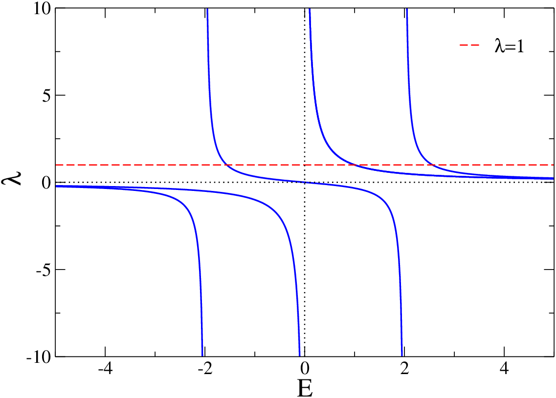
We stress that extracting the full energy spectrum of the pair based on the effective model, for a fixed value of the interaction strength , is computationally demanding as becomes large. The effective model is instead very efficient, as compared to the exact diagonalization, when we look at the properties of the pair as a function of the interaction strength , for a fixed value of the total energy . This is exactly the situation that we will be interested in below.
IV Absence of 2D delocalization transitions for the pair
Numerical evidence of 2D Anderson transition for two particles obeying the Anderson-Hubbard model in two dimensions was first reported Ortuño and Cuevas 1999 on the basis of transmission-amplitude calculations McKinnon and Kramer 1983 performed on rectangular strips of length and variable width up to . For a pair with zero total energy and for interaction strength , the delocalization transition was found to occur for . The result was also confirmed Cuevas 1999 from the analysis of the energy-level statistics, although with slightly different numbers.
The existence of a 2D mobility edge for the pair was also reported in Ref. Roemer et al. 1999, where a decimation method was employed to compute the critical disorder strength as a function of the interaction strength , based on lattices of similar sizes. For , a pair with zero total energy was shown to undergo an Anderson transition at .
Below we verify the existence of the 2D delocalization transition of the pair, following the procedure developed in Ref. Stellin and Orso 2019. In order to compare with the previous numerical predictions, we set and . We consider a rectangular strip of dimensions , with , containing lattice sites. In order to minimize finite-size effects, the boundary conditions on the single-particle Hamiltonian are chosen periodic in the orthogonal direction () and open along the transmission axis (). We rewrite the rhs of Eq. (6) as
| (10) |
where is the Green’s function (e.g. the resolvent) of the single-particle Anderson Hamiltonian (1), being the identity matrix. Due to the open boundary conditions along the longitudinal direction, the Anderson Hamiltonian possesses a block tridiagonal structure, each block corresponding to a transverse section of the grid. This structure can be exploited to efficiently compute the Green’s function in Eq. (10) via matrix inversion. In this way the total number of elementary operations needed to compute the matrix scales as , instead of , as naively expected from the rhs of Eq. (6).
Once computed the matrix of the effective model, we use it to evaluate the logarithm of the transmission amplitude between two transverse sections of the strip as a function of their relative distance :
| (11) |
In Eq. (11) is the Green’s function associated to with and the sum is taken over the sites of the two transverse sections.

For each disorder realization, we evaluate at regular intervals along the bar and apply a linear fit to the data, . For a given value of the interaction strength, we evaluate the (disorder-averaged) Lyapunov exponent as , where is the average of the slope. We then infer the localization properties of the system from the behavior of the reduced localization length, which is defined as . In the metallic phase increases as increases, whereas in the insulating phase the opposite trend is seen. At the critical point, becomes constant for values of sufficiently large. Hence the critical point of the Anderson transition can be identified by plotting the reduced localization length versus for different values of the transverse size and looking at their common crossing points.
In Fig. 2 we show the reduced localization length as a function of the interaction strength for increasing values of the strip width, ranging from to . The length of the grid is fixed to . Notice that, since , the reduced localization length is an even function of the interaction strength, . We see that exhibits a nonmonotonic dependence on , as previously found in one Frahm 2016 and in three Stellin and Orso 2019 dimensions. In particular, interactions favor the delocalization of the pair, the effect being more pronounced near . We also notice from Fig. 2 that the curves corresponding to different values of intersect each others around , suggesting a possible phase transition, as previously reported in Ref. Ortuño and Cuevas 1999; Roemer et al. 1999. A closer inspection of the data, however, reveals that the crossing points are spread out in the interval ; in particular, they drift to stronger interactions as the system size increases, in analogy with the three-dimensional case Stellin and Orso 2019.

A key question is whether a further increase of the strip’s width will only cause a (possibly large) shift of the critical point, or rather, the localized phase will ultimately take over for any value of the interaction strength. To answer this question, we have performed additional calculations using larger grids, corresponding to . In order to guarantee a sufficiently large aspect ratio, the length of the bar was fixed to . The obtained results are displayed in Fig.3. We notice that the crossing points have completely disappeared and the pair localizes in an infinite lattice irrespectively of the specific value of . This leads us to conclude that the results of Refs. Ortuño and Cuevas 1999; Roemer et al. 1999 were plagued by severe finite-size effects, due to the limited computational ressources, and no Anderson transition can actually take place for a pair in a disordered lattice of infinite size.
V Pair localization length
Although the pair cannot fully delocalize in two dimensions, interactions can lead to a drastic enhancement of the two-particle localization length. This quantity can be estimated using the one-parameter scaling ansatz , stating that the reduced localization length depends solely on the ratio between two quantities: the width of the strip and a characteristic length , which instead depends on the model parameters and on the total energy of the pair (but not on the system sizes ). This latter quantity coincides, up to a multiplicative numerical constant , with the pair localization length, .
We test the scaling ansatz for our effective model (5) using the numerical data for displayed in Fig.3, corresponding to the largest system sizes. Let , with , be the values of the interaction strength used to compute the reduced localization length (in our case ). We then determine the corresponding unknown parameters through a least squares procedure, following the procedure developed in Ref. McKinnon and Kramer 1983. Plotting our data in the form vs results in multiple data curves, each of them containing three data points connected by straight lines (corresponding to linear interpolation). Let be one of the numerical values available for the reduced localization length. The horizontal line will generally intersect some of these curves. We find convenient to introduce a matrix which keeps track of such events: if the curve is crossed, we set and call the corresponding point; otherwise we set . The unknown parameters are then obtained by minimizing the variance of the difference , yielding the following set of equations (see Ref. McKinnon and Kramer 1983 for a detailed derivation):
| (12) |
where is the total number of crossing points obtained for each value. Equation (12) is of the form and can be easily solved. Notice however that the solution is not unique because the matrix is singular. Indeed the correlation length is defined up to a multiplicative constant, , implying that is defined up to an additive constant, .

In Fig.4 we verify the correctness of the scaling ansatz, by plotting the reduced localization length as a function of the ratio , where is obtained from the solution of Eq. (12). We see that our numerical data for different values of the interaction strength and system size do collapse on a single curve, thus confirming the scaling hypothesis. In the main panel of Fig. 5 we plot the unnormalized localization length of the pair as a function of the interaction strength. We see that varies over more than three orders of magnitude in the interval of values considered. In particular, for weak interactions the growth is approximately exponential in , as highlighted by the semi-logarithmic plot. Based on analytical arguments, Imry suggested Imry 1995 that the localization length of the pair in the weakly interacting regime should obey the relation , where is the single-particle localization length of the Anderson model and is a numerical factor. A possible reason of the discrepancy is that the cited formula might apply only for relatively modest values of the interaction strength, which were not explored in our numerics. Further work will be needed to address this point explicitly.

The constant , allowing to fix the absolute scale of the localization length of the pair, is independent of the interaction strength. Its numerical value can in principle be inferred by fitting the data in the strongly localized regime, according to
| (13) |
where is a number. In our case the most localized states are those at weak interactions, where the reduced localization length takes its minimum value. For each values falling in this region, we fit our numerical data according to Eq. (13), yielding . The estimate of the multiplicative constant, which is defined as , is displayed in the inset of Fig. 5. Since the estimate of does not saturates for small , we conclude that, even for the weakest interactions and the largest system sizes considered, the pair has not yet entered the strongly localized regime underlying Eq. (13). This asymptotic regime is typically achieved for , whereas our smallest value of the reduced localization length is . From the inset of Fig. 5 we also see that increases as diminishes, suggesting that the result obtained for actually provides a lower bound for the multiplicative constant. This allows us to conclude that .
VI Generality of the obtained results

In Sec. IV we have shown that all pair states with total energy are localized for . A natural question is whether the localization scenario changes at nonzero energy or at weak disorder. Let us consider the two cases separately. Our numerical results indicate that, for any values of and system size , the reduced localization length always takes its maximum value for :
| (14) |
As an example, in Fig.6 we plot as a function of the interaction strength, for and for different negative values of the energy (results for positive energies are simply obtained from the corresponding data at energy by reversing the sign of the interaction strength, ). All calculations are performed on a strip with constant sizes and . When combined with the finite-size scaling analysis, the inequality (14) implies that the pair remains localized for any nonzero energy with an even shorter localization length, thus excluding a delocalization transition. The above inequality expresses the general fact that the pair can better spread when its total energy lies in the middle of the noninteracting two-particle energy spectrum. For instance, in three dimensions, where genuine Anderson transitions for the pair do occur, we found Stellin and Orso 2020 that metallic regions in the interaction-disorder plane become progressively insulating as the energy of the pair departs from zero.
We note from Fig.6 that all data curves with have absolute minimum at . Moreover, the largest enhancement of the reduced localization length takes place for weaker interactions as increases. These are specific features of scattering states, whose energy lies inside the noninteracting two-body energy spectrum, as already observed in one Frahm 2016 and in three Stellin and Orso 2020 dimensions. In the asymptotic regime , pairs behave as pointlike molecules and the effective model takes the form of a single-particle Anderson model, as discussed in Ref. Stellin and Orso 2020, which again precludes the possibility of a delocalization transition in two dimensions.
Let us now discuss whether an Anderson transition for the pair can appear for weak disorder at fixed total energy, . The effective single-particle model possesses both time reversal and spin rotational symmetries, suggesting that belongs to the same (orthogonal) universality class of the Anderson model . In Ref. Stellin and Orso 2019 we showed numerically that, in three dimensions, the Anderson transition for a pair with zero energy yields critical exponents in agreement with the predictions of the orthogonal class. Since 2D Anderson transitions are generally forbidden in the orthogonal class, one expects that the pair is localized for any finite disorder. For this reason, the previous claims of 2D delocalization transitions for two particles are puzzling. Our numerics shows explicitly that these results were biased by strong finite-size effects and there is no evidence of violation of the conventional localization scenario.
From the numerical point of view, the observation of the asymptotic 2D scaling behavior for required large system sizes as compared to the 3D case studied in Ref. Stellin and Orso 2019, where the finite-size scaling analysis was limited to system sizes up to . Verifying numerically the absence of the 2D transition for weaker disorder is very challenging, because the reduced localization length will exhibit an apparent crossing for even larger values of as diminishes. To appreciate this point, we have repeated the same finite-size scaling analysis for and plotted the results in Fig.7. We see that, already for , the pair is localized for any values of the interaction strength, whereas for the same asymptotic behavior is reached for larger system sizes, between and .

VII Conclusion and outlook
Based on an efficient mapping of the two-body Schrodinger equation, we have addressed the localization properties of two bosons or two spin 1/2 fermions in a singlet state obeying the 2D Anderson-Hubbard model. We have found that no interaction-induced Anderson transition occurs for disordered lattices of infinite size in contrast with previous numerical works, which we have shown to be biased by finite-size effects. In this way we reconcile the numerics with the one-parameter scaling theory of localization, predicting the absence of one-particle Anderson transition in two dimensions, in the presence of both time reversal and spin rotational symmetries. Moreover, we found that the pair localization length exhibits a nonmonotonic behavior as a function of , characterized by an exponential growth for weak interactions.
We point out that the absence of the 2D mobility edge for the two-particle system has been proven for the case of contact interactions; similar conclusions should apply also for short but finite-range interactions. The case of true long-range (e.g Coulomb) interactions is conceptually different and can lead to opposite conclusions Cuevas 1999; Shepelyansky 2000. From the above discussion, we also expect that the 2D delocalization transition will appear when the two particles are exposed to spin-orbit couplings, driving the system towards the symplectic universality class, where single-particle metal-insulator transitions are generally allowed even in two dimensions Evers and Mirlin 2008.
An interesting and compelling problem is to investigate the implications of our results for a 2D system at finite density of particles, where many-body delocalization transitions have instead been observed, both numerically and experimentally, in the strongly interacting regime. We expect that, in the zero density limit, the many-body mobility edge disappears, irrespective of the bosonic or fermionic statistics of the two particles. Another interesting direction is to generalize our numerical approach to study the effect of disorder on the transport and spectral properties of excitons in 2D semiconductors Kirichenko and Stephanovich 2019.
ACKNOWLEDGEMENTS
We acknowledge D. Delande, K. Frahm, C. Monthus, S. Skipetrov and T. Roscilde for fruitful discussions. This project has received funding from the European Union’s Horizon 2020 research and innovation programme under the Marie Sklodowska-Curie grant agreement No 665850. This work was granted access to the HPC resources of CINES (Centre Informatique National de l’Enseignement Supérieur) under the allocations 2017-A0020507629, 2018-A0040507629, 2019-A0060507629 and 2020-A0080507629 supplied by GENCI (Grand Equipement National de Calcul Intensif).
References
- Anderson (1958) P. W. Anderson, Phys. Rev. 109, 1492 (1958).
- Wiersma et al. (1997) D. S. Wiersma, P. Bartolini, A. Lagendijk, and R. Righini, Nature (London) 390, 671 (1997).
- Störzer et al. (2006) M. Störzer, P. Gross, C. M. Aegerter, and G. Maret, Phys. Rev. Lett. 96, 063904 (2006).
- Schwartz et al. (2007) T. Schwartz, G. Bartal, S. Fishman, and B. Segev, Nature (London) 446, 52 (2007).
- Lahini et al. (2008) Y. Lahini, A. Avidan, F. Pozzi, M. Sorel, R. Morandotti, D. N. Christodoulides, and Y. Silberberg, Phys. Rev. Lett. 100, 013906 (2008).
- Hu et al. (2008) H. Hu, A. Strybulevych, J. H. Page, S. E. Skipetrov, and B. A. van Tiggelen, Nat. Phys. 4, 945 (2008).
- Chabanov et al. (2000) A. A. Chabanov, M. Stoytchev, and A. Z. Genack, Nature (London) 404, 850 (2000).
- Billy et al. (2008) J. Billy, V. Josse, Z. Zuo, A. Bernard, B. Hambrecht, P. Lugan, D. Clément, L. Sanchez-Palencia, P. Bouyer, and A. Aspect, Nature (London) 453, 891 (2008).
- Roati et al. (2008) G. Roati, C. d’Errico, L. Fallani, M. Fattori, C. Fort, M. Zaccanti, G. Modugno, M. Modugno, and M. Inguscio, Nature (London) 453, 895 (2008).
- Altland and Zirnbauer (1997) A. Altland and M. R. Zirnbauer, Phys. Rev. B 55, 1142 (1997).
- Evers and Mirlin (2008) F. Evers and A. D. Mirlin, Rev. Mod. Phys. 80, 1355 (2008).
- Kondov et al. (2011) S. S. Kondov, W. R. McGehee, J. J. Zirbel, and B. DeMarco, Science 334, 66 (2011).
- Jendrzejewski et al. (2012) F. Jendrzejewski, A. Bernard, K. Muller, P. Cheinet, V. Josse, M. Piraud, L. Pezzé, L. Sanchez-Palencia, A. Aspect, and P. Bouyer, Nat. Phys. 8, 398 (2012).
- Semeghini et al. (2015) G. Semeghini, M. Landini, P. Castilho, S. Roy, G. Spagnolli, A. Trenkwalder, M. Fattori, M. Inguscio, and G. Modugno, Nat. Phys. 11, 554 (2015).
- Yedjour and Van Tiggelen (2010) A. Yedjour and B. Van Tiggelen, Eur. Phys. J. D 59, 249 (2010).
- Piraud et al. (2014) M. Piraud, L. Sanchez-Palencia, and B. van Tiggelen, Phys. Rev. A 90, 063639 (2014).
- Delande and Orso (2014) D. Delande and G. Orso, Phys. Rev. Lett. 113, 060601 (2014).
- Fratini and Pilati (2015a) E. Fratini and S. Pilati, Phys. Rev. A 91, 061601(R) (2015a).
- Pasek et al. (2015) M. Pasek, Z. Zhao, D. Delande, and G. Orso, Phys. Rev. A 92, 053618 (2015).
- Fratini and Pilati (2015b) E. Fratini and S. Pilati, Phys. Rev. A 92, 063621 (2015b).
- Pasek et al. (2017) M. Pasek, G. Orso, and D. Delande, Phys. Rev. Lett. 118, 170403 (2017).
- Orso (2017) G. Orso, Phys. Rev. Lett. 118, 105301 (2017).
- Kravchenko et al. (1994) S. V. Kravchenko, G. V. Kravchenko, J. E. Furneaux, V. M. Pudalov, and M. D’Iorio, Phys. Rev. B 50, 8039 (1994).
- Punnoose and Finkel’stein (2005) A. Punnoose and A. M. Finkel’stein, Science 310, 289 (2005).
- Knyazev et al. (2008) D. A. Knyazev, O. E. Omel’yanovskii, V. M. Pudalov, and I. S. Burmistrov, Phys. Rev. Lett. 100, 046405 (2008).
- Gornyi et al. (2005) I. V. Gornyi, A. Mirlin, and D. G. Polyakov, Phys. Rev. Lett. 95, 206603 (2005).
- Basko et al. (2006) D. M. Basko, I. L. Aleiner, and B. L. Altshuler, Ann. Phys. 321, 1126 (2006).
- Nandkishore and Huse (2015) R. Nandkishore and D. A. Huse, Annu. Rev. Condens. Matter Phys. 6, 15 (2015).
- Alet and Laflorencie (2018) F. Alet and N. Laflorencie, Comptes Rendus Physique 19, 498 (2018).
- Abanin et al. (2019) D. A. Abanin, E. Altman, I. Bloch, and M. Serbyn, Rev. Mod. Phys. 91, 021001 (2019).
- Schreiber et al. (2015) M. Schreiber, S. S. Hodgman, P. Bordia, H. P. Lüschen, M. H. Fischer, R. Vosk, E. Altman, U. Schneider, and I. Bloch, Science 349, 842 (2015).
- Rispoli et al. (2019) M. Rispoli, A. Lukin, R. Schittko, S. Kim, M. E. Tai, J. Léonard, and M. Greiner, Nature 573, 385 (2019).
- Oganesyan and Huse (2007) V. Oganesyan and D. A. Huse, Phys. Rev. B 75, 155111 (2007).
- Luitz et al. (2015) D. J. Luitz, N. Laflorencie, and F. Alet, Phys. Rev. B 91, 081103(R) (2015).
- Michal et al. (2014) V. P. Michal, B. L. Altshuler, and G. V. Shlyapnikov, Phys. Rev. Lett. 113, 045304 (2014).
- Andraschko et al. (2014) F. Andraschko, T. Enss, and J. Sirker, Phys. Rev. Lett. 113, 217201 (2014).
- Mondaini and Rigol (2015) R. Mondaini and M. Rigol, Phys. Rev. A 92, 041601(R) (2015).
- Reichl and Mueller (2016) M. D. Reichl and E. J. Mueller, Phys. Rev. A 93, 031601(R) (2016).
- Prelovšek et al. (2016) P. Prelovšek, O. S. Barišić, and M. Žnidarič, Phys. Rev. B 94, 241104(R) (2016).
- Zakrzewski and Delande (2018) J. Zakrzewski and D. Delande, Phys. Rev. B 98, 014203 (2018).
- Hopjan and Heidrich-Meisner (2020) M. Hopjan and F. Heidrich-Meisner, Phys. Rev. A 101, 063617 (2020).
- (42) U. Krause, T. Pellegrin, P. W. Brouwer, D. A. Abanin, and M. Filippone, eprint arXiv:1911.11711.
- Yao and Zakrzewski (2020) R. Yao and J. Zakrzewski, Phys. Rev. B 102, 014310 (2020).
- De Roeck et al. (2016) W. De Roeck, F. Huveneers, M. Müller, and M. Schiulaz, Phys. Rev. B 93, 014203 (2016).
- De Roeck and Huveneers (2017) W. De Roeck and F. Huveneers, Phys. Rev. B 95, 155129 (2017).
- Choi et al. (2016) J.-y. Choi, S. Hild, J. Zeiher, P. Schauß, A. Rubio-Abadal, T. Yefsah, V. Khemani, D. A. Huse, I. Bloch, and C. Gross, Science 352, 1547 (2016).
- Wahl et al. (2019) T. B. Wahl, A. Pal, and S. H. Simon, Nature Physics 15, 164 (2019).
- (48) A. Geissler and G. Pupillo, eprint arXiv:1909.09247.
- De Tomasi et al. (2019) G. De Tomasi, F. Pollmann, and M. Heyl, Phys. Rev. B 99, 241114 (2019).
- Thomson and Schiró (2018) S. J. Thomson and M. Schiró, Phys. Rev. B 97, 060201(R) (2018).
- Théveniaut et al. (2020) H. Théveniaut, Z. Lan, G. Meyer, and F. Alet, Phys. Rev. Research 2, 033154 (2020).
- Stellin and Orso (2019) F. Stellin and G. Orso, Phys. Rev. B 99, 224209 (2019).
- Stellin and Orso (2020) F. Stellin and G. Orso, Phys. Rev. Research 2, 033501 (2020).
- Shepelyansky (1994) D. L. Shepelyansky, Phys. Rev. Lett. 73, 2607 (1994).
- Weinmann et al. (1995) D. Weinmann, A. Müller-Groeling, J.-L. Pichard, and K. Frahm, Phys. Rev. Lett. 75, 1598 (1995).
- von Oppen et al. (1996) F. von Oppen, T. Wettig, and J. Müller, Phys. Rev. Lett. 76, 491 (1996).
- Frahm (1999) K. M. Frahm, Eur. Phys. J. B 10, 371 (1999).
- Roemer et al. (2001) R. A. Roemer, M. Schreiber, and T. Vojta, Physica E 9, 397 (2001).
- Krimer et al. (2011) D. Krimer, R. Khomeriki, and S. Flach, Jetp Lett. 94, 406 (2011).
- Dias and Lyra (2014) W. S. Dias and M. L. Lyra, Physica A 411, 35 (2014).
- Lee et al. (2014) C. Lee, A. Rai, C. Noh, and D. G. Angelakis, Phys. Rev. A 89, 023823 (2014).
- Krimer and Flach (2015) D. O. Krimer and S. Flach, Phys. Rev. B 91, 100201(R) (2015).
- Frahm (2016) K. M. Frahm, Eur. Phys. J. B 89, 115 (2016).
- Thongjaomayum et al. (2019) D. Thongjaomayum, A. Andreanov, T. Engl, and S. Flach, Phys. Rev. B 100, 224203 (2019).
- Thongjaomayum et al. (2020) D. Thongjaomayum, S. Flach, and A. Andreanov, Phys. Rev. B 101, 174201 (2020).
- Lahini et al. (2010) Y. Lahini, Y. Bromberg, D. N. Christodoulides, and Y. Silberberg, Phys. Rev. Lett. 105, 163905 (2010).
- Chattaraj and Krems (2016) T. Chattaraj and R. V. Krems, Phys. Rev. A 94, 023601 (2016).
- Wiater et al. (2017) D. Wiater, T. Sowiński, and J. Zakrzewski, Phys. Rev. A 96, 043629 (2017).
- Toikka (2020) L. A. Toikka, Phys. Rev. B 101, 064202 (2020).
- Malishava et al. (2020) M. Malishava, I. Vakulchyk, M. Fistul, and S. Flach, Phys. Rev. B 101, 144201 (2020).
- Mujal et al. (2019) P. Mujal, A. Polls, S. Pilati, and B. Juliá-Díaz, Phys. Rev. A 100, 013603 (2019).
- Schmidtke et al. (2017) D. Schmidtke, R. Steinigeweg, J. Herbrych, and J. Gemmer, Phys. Rev. B 95, 134201 (2017).
- Imry (1995) Y. Imry, Europhys. Lett. 30, 405 (1995).
- Borgonovi and Shepelyansky (1995) F. Borgonovi and D. L. Shepelyansky, Nonlinearity 8, 877 (1995).
- Ortuño and Cuevas (1999) M. Ortuño and E. Cuevas, Europhysics Letters 46, 224 (1999).
- Cuevas (1999) E. Cuevas, Phys. Rev. Lett. 83, 140 (1999).
- Roemer et al. (1999) R. A. Roemer, M. Leadbeater, and M. Schreiber, Ann. Phys. (Leipzig) 8, 675 (1999).
- Burmistrov et al. (2014) I. S. Burmistrov, I. V. Gornyi, and A. D. Mirlin, Phys. Rev. B 89, 035430 (2014).
- Dufour and Orso (2012) G. Dufour and G. Orso, Phys. Rev. Lett. 109, 155306 (2012).
- Orso et al. (2005) G. Orso, L. P. Pitaevskii, S. Stringari, and M. Wouters, Phys. Rev. Lett. 95, 060402 (2005).
- McKinnon and Kramer (1983) A. McKinnon and B. Kramer, Z. Phys. B 53, 1 (1983).
- Shepelyansky (2000) D. L. Shepelyansky, Phys. Rev. B 61, 4588 (2000).
- Kirichenko and Stephanovich (2019) E. V. Kirichenko and V. A. Stephanovich, Phys. Chem. Chem. Phys. 21, 21847 (2019).