Emulation of magneto-optic Faraday effect using ultracold atoms

Emulation of quantum condensed-matter systems using ultracold atoms is an active area in the studies of quantum simulations [1, 2, 3, 4]. This is because ultracold atoms can provide a versatile platform with a series of advantages: (i) The nontrivial interplay or external fields can be designed by the setup of the laser-atom interaction that can bring novel physics [5, 6]. (ii) The high controllability of the synthetic interplay and fields has promising applications such as exploring intriguing phase transitions [7, 8, 9] and critical phenomena [10, 11]. (iii) The absence of the disorder effect or impurities makes the well-isolated system ideally clean [12], and thereby facilitates the investigation for unraveling complex phenomena. Based on these features, a variety of emulations using ultracold atoms have been successfully proposed in a broad range of interesting topics, for instance the ferromagnetism [13], quantum Hall effect [14, 15, 16, 17], atomtronic circuit [18, 19] and its hysteresis [20], atom transistor [21], and optical solenoid associated with magnetic flux [22].

In condensed-matter physics, the magneto-optic effect is a fundamental but broad concept in the magnetic mediums. It has been known that the transverse conductivity plays a crucial role in the magneto-optic effect [23], which can be introduced by the interplay of the band exchange splitting and spin-orbit coupling in the magnetic medium [24]. When the light transmits from vacuum to the medium, the presence of the transverse conductivity hybrids the two polarized components of the photons and imposes a coherent phase to them during the light propagation. As the result, the polarized angle of the reflected and forward scattered light fields deviates from the one of the incident light, respectively known as the magneto-optic Kerr effect (MOKE) and Faraday effect (MOFE). In recent studies, the magneto-optic effect can also arise by virtue of the topological Hall effect, in which the rotated polarized angle is related to the topological invariant, known as the topological magneto-optic effect [25, 26, 27].

However, a great deal of experiment advances on the magneto-optic effect has constituted the focus of major efforts to MOKE rather than MOFE. This is because the distinct measurement of MOFE has been elusive so far in ordinary magnetic mediums. In MOKE, the rotation of the polarized angle, which is the prominent feature of the magneto-optic effect, is affected by the medium boundary condition of the light reflection. By starkly contrast in MOFE, it accumulates during the light propagation in mediums. For the sake of the photon absorption by the medium, MOFE is generally expected to be detected in ultra-thin films. The magnitude of the rotated polarized angle thus dramatically drops in thinner films, and therefore the salient signal of MOFE is challengingly attainable in real experiments. On the other hand as mentioned, the emulation using ultracold atoms has advantages in realizing artificial physics system with controllable manipulations. This motivates us to search a possible alternative routine for studying MOFE via the emulation in the atomic gases, instead of the challenged detection in conventional solid-state systems.

In this work, we propose such a proposal for emulating MOFE using ultracold atoms. The mechanism for the synthetic MOFE relies on the light-atom interplay, which stands out from the conventional physics picture and provides full controllability as well as detectable signals with existing techniques. The paper is organized as follows. In section 2, we present the detailed model of the emulation. For simplicity we firstly consider the model at resonance to extract the physics picture, and in section 3 without loss of generality, the detuned case is investigated. In section 4, we address the relevant practical considerations and possible implementation of the proposal. In section 5, we summarize the work.

We consider the bosons with two internal levels that are denoted as pseudo-spins $\uparrow$ and $\downarrow$. In ultracold Bose gases, the atomic cloud can be loaded into two reservoirs separated by a mesoscopic channel [28, 29, 30, 31]. By preparing the two reservoirs with a number imbalance, the atomic current can be observed through the channel, and the hydrodynamics of the atomic cloud density is semi-classically refined by the equation $\partial_{t}n+{\bf v}\cdot\nabla n=0$ [32]. The linear dispersion shares the similarity of the light propagation. Furthermore, in Bose gases, specifically the Bose-Einstein condensate (BEC), the wave function of different pseudo-spins are orthogonal, exhibiting the same property of the polarized components of the light. Therefore, the atomic transport process inspires us to draw an analogy to the light field in terms of the bosonic cloud. Despite that the atomic ensemble is totally different from the magnetic mediums, the phenomenal and intrinsic similarities can reveal the fundamental physics at the macroscopic level, which is the focus of quantum simulation.

The experimental setup is illustrated in Figure 1(a). We suppose the atomic cloud is prepared in the BEC phase. In the channel between the reservoirs, the atomic cloud can be approximately regarded as being confined in the harmonic trap potential $V_{\rm trap}({\bf r})=\frac{1}{2}m\omega_{\rm trap}(x^{2}+y^{2})$. In the section normal to the $z$ direction, the wave function of the ground state can be given by

where $l_{0}=\sqrt{\hbar/(m\omega_{\rm trap})}$ [33]. Along the $z$ direction, the atomic cloud flows at a center-of-mass (COM) velocity $v_{\rm cm}$.

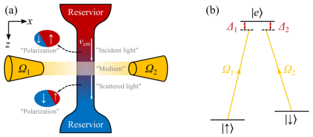
As the spin of atoms mimics the polarization of light, we implement counter-propagating lasers along the $x$ direction, which drives a Raman transition between the two spins via an auxiliary excited levels. In this way, the artificial transverse conductivity can be equivalently generated by laser fields that couples different spins, and the laser-atom interacting region will play the role of the “medium”. The transition is sketched in Figure 1(b). At low temperature, we assume the velocity fluctuation is much smaller than the laser field strength. In the COM reference frame, such a $\Lambda$ system is governed by the following Hamiltonian,

Here $|\lambda\rangle$ with $\lambda=\uparrow,\downarrow,e$ denote the spin-$\uparrow,\downarrow$ and excited states, respectively. $\Gamma_{\uparrow,\downarrow,e}$ are their corresponding level energies. $\hat{\Omega}_{\alpha=1,2}({\bf r})\equiv M_{\alpha}({\bf r})e^{ik_{\alpha}x}$ where $M_{\alpha}({\bf r})$ characterizes the laser field mode followed with the frequency $\omega_{\alpha}$ as well as the standing-wave vector $k_{\alpha}$. $H.c.$ stands for the Hermitian conjugation. We can assume the general form of the wave function for the three-level system as $|\psi\rangle=\sum_{\lambda}c_{\lambda}e^{-i\Gamma_{\lambda}/\hbar}|\lambda\rangle$. According to the Schrödinger equation $i\partial_{t}|\psi\rangle=H|\psi\rangle$, the coefficient $c_{\lambda}$ satisfies the following equations,

Here we have denoted the detuning as $\Delta_{1}=\Gamma_{e}-\Gamma_{\uparrow}-\hbar\omega_{1}$ and $\Delta_{2}=\Gamma_{e}-\Gamma_{\downarrow}-\hbar\omega_{2}$. For simplicity without loss of generality, we normalize the atomic densities by the total atomic number of the condensate. Thus the coefficient $c_{\lambda}$ obeys the constraint $\sum_{\lambda}|c_{\lambda}|^{2}=1$ due to the number conversation.

In order to give a simple physics picture for our proposal, we firstly consider the resonance condition $\Delta_{1}=\Delta_{2}=0$. The atoms are initially prepared to reside in the two spin states that host the lowest energy. Due to spontaneous breaking the $U(1)$ symmetry, the BEC hosts distinguished phases for each spins [34]. Thereby, the initial state of the spinful system can be assumed as the form $|\psi_{0}\rangle=\cos\theta\mbox{$|\uparrow\rangle$}+\sin\theta e^{i\varphi}\mbox{$|\downarrow\rangle$}$. Here $\theta$ characterizes the number imbalance of spins, and $\varphi$ describes the relative phase between the two spins. The solution to Eq.(3) is then given as follows,

Here the dimensionless function is written as $F({\bf r})=[\hat{\Omega}_{1}({\bf r})\cos\theta+\hat{\Omega}_{2}({\bf r})e^{i\varphi}\sin\theta+H.c.]/[2\hat{\Omega}_{R}({\bf r})]$. $\hat{\Omega}_{R}({\bf r})=\sqrt{|\hat{\Omega}_{1}({\bf r})|^{2}+|\hat{\Omega}_{2}({\bf r})|^{2}}$ is the Rabi frequency.

For simplicity, we postulate the laser modes $M_{1,2}({\bf r})$ to be slowly varied along the $x$ direction in the atomic cloud. As the laser fields are applied along the $x$ direction, the atomic transition driven by them involves no momentum transfer in the $z$ direction, and hence does not affect the atomic transport. In the laboratory frame, the Rabi frequency can be approximately expanded as $\hat{\Omega}_{R}({\bf r}_{\rm cm}+{\bf r}^{\prime})\approx\hat{\Omega}_{R}({\bf r}_{\rm cm})+{\bf r}^{\prime}\cdot\nabla\hat{\Omega}_{R}({\bf r}_{\rm cm})$. Here the COM coordinate ${\bf r}_{\rm cm}=v_{\rm cm}t\hat{\bf e}_{z}$ with $\hat{\bf e}_{x,y,z}$ being the unit vector. Since the laser fields are spatially uniform along the trajectory direction, quantities that depend only on ${\bf r}_{\rm cm}$ can be regarded as constants hereafter. We denote the gradient of the laser field as $\nabla\hat{\Omega}_{R}({\bf r}_{\rm cm})\equiv A\hat{\bf e}_{x}$.

We remark that the gradient potential $A$ can be attainable in practice, for instance by using Gaussian beams whose center deviates from the atomic COM trajectory, or the tilted potential that is widely applied in the technique of laser-assisted tunneling [14, 15].

In a steady transport case, the atomic current is incompressible along the trajectory direction. The density per unit of length along the $z$ direction can thus be obtained by $n_{\lambda}=\int|c_{\lambda}\psi({\bf r})|^{2}dxdy$, where the spatial distribution $\psi({\bf r})$ has been given in Eq.(1). In particular, for spin-$\uparrow$ atoms, it is expressed as

We suppose the spatial scale of the atomic cloud is tremendously larger than the laser wavelengths, i.e. $k_{1}l_{0},k_{2}l_{0}\gg 1$. By using the following mathematical relation,

the rapid spatial modulated terms such as $\cos(k_{1}x)$ and $\cos(k_{2}x+\varphi)$ in $F({\bf r})$ of Eq.(5) will be averaged to exponentially vanish when integrating out the spatial coordinates. Then we have

where the time-dependent functions defined as

and $\mathcal{F}=(\Omega_{1}^{2}\cos^{2}\theta+\Omega_{2}^{2}\sin^{2}\theta)/(2\Omega_{R}^{2})$. We have denoted $\Omega_{1,2}=M_{1,2}({\bf r}_{\rm cm})$ and $\Omega_{R}=\hat{\Omega}_{R}({\bf r}_{\rm cm})$. The decay time $\tau_{c}$ is defined as

Likewise, the density evolutions of spin-$\downarrow$ and excited-state atoms are obtained as

From Eqs.(7), (11) and (12), one can see that in the presence of the laser field gradient $A$, the Rabi oscillations are exponentially suppressed. Similar phenomena can be evidenced by experiments yet in a two-level system [35]. The atomic cloud will evolve to a steady state in which the densities of spin $\uparrow$ and $\downarrow$ saturate to

The dynamic evolutions are shown in Figure 2(a) and (b) for different initial setups. For simplicity, we have assumed the atomic cloud in motion enters the laser region at $t=0$, and leaves it after the cloud fully evolved to the steady state. It can be guaranteed by preparing the width of the laser region $L>v_{\rm cm}\tau_{c}$.

As we use the bosonic atoms to represent the light field, the polarized angle $\phi$ of the emulated light field is defined by the atomic densities,

which is time dependent. In particular, the polarized angle of the incident light is expressed as $\phi_{\rm in}=\tan^{-1}(\tan^{2}\theta)$, while for the scattered light is calculated by $\phi_{\rm sc}=\tan^{-1}[n_{\downarrow}(\infty)/n_{\uparrow}(\infty)]$ (c.f. Eq.(13)). In Figure 2(c), we can see the polarized angle is changed after the light passes through the emulated medium, exhibiting the manifest feature of MOFE. The signal of the artificial MOFE (i.e. the rotated polarized angle) not only depends on the parameter $\theta$ of initial setups, but is also controllable by the laser field strengths $\Omega_{1,2}$.

The resonance condition used in the above discussions will introduce the additional heating effect that are frustrated to the practical experiments such as suppressing the lifetime of ultracold atoms [36]. However, we remark that the resonance condition in the $\Lambda$ system is not necessary, instead the proposal still works when the laser-atom interaction is prepared with a detuning $\Delta_{1}=\Delta_{2}=\Delta\neq 0$. It has a crucial advantage that, at the fully far detuned regime (i.e. $\Delta\gg|\hat{\Omega}_{1,2}({\bf r})|$), the heating effect can prominently suppressed and thereby facilitates the realization of the proposal.

At the detuned case, the evolutions of the atomic densities for spin $\uparrow$ and $\downarrow$ share the same forms of Eqs.(7) and (11), but the time-dependent functions are instead rewritten as (see A)

Here the Rabi oscillations are split into two branches whose frequencies are expresses as $\hat{\Omega}_{R}^{\pm}({\bf r})=\Delta/2\pm\sqrt{|\hat{\Omega}_{1}({\bf r})|^{2}+|\hat{\Omega}_{2}({\bf r})|^{2}+\Delta^{2}/4}$. The dimensionless constant $\mathcal{F}^{\prime}=(\Omega_{1}^{2}\cos^{2}\theta+\Omega_{2}^{2}\sin^{2}\theta)/[2(\Omega_{R}^{+}+\Omega_{R}^{-})^{2}]$. We have denoted $\Omega_{R}^{\pm}=\pm\hat{\Omega}_{R}^{\pm}({\bf r}_{\rm cm})$, $A_{\pm}=\pm\nabla_{x}\hat{\Omega}_{R}^{\pm}({\bf r}_{\rm cm})$, $\tau_{c\pm}=2\hbar/(A_{\pm}l_{0})$, and $\widetilde{\tau}_{c}^{-1}=\tau_{c+}^{-1}+\tau_{c-}^{-1}$. It is easy to demonstrated that $K_{1,2}(t)$ reduces to the form given in Eqs.(8) and (9) at resonance $\Delta=0$. The evolutions are plotted in Figure 3(a) and (b). Likewise as in a similar way to the resonance condition, the polarized angle of the incident light is shifted after passing through the medium, as shown in Figure 3(c).

We comment that the decay time $\tau_{c+}$ and $\tau_{c-}$ are indeed identical. This is because the spatial dependence of $\hat{\Omega}_{R}^{\pm}({\bf r})$ originates from the laser field modes $M_{1,2}({\bf r})$, and hence their gradients $A_{\pm}$ are equal to each other. In comparison between Figure 2(c) and Figure 3(c), we find that the rotated polarized angles is insensitive to the detuning $\Delta$. This is because in the steady state, $\Delta$ only affects the Rabi frequencies $\hat{\Omega}_{R}^{\pm}({\bf r})$, which is nearly canceled out in the calculation using Eq.(14).

In summary, we propose a scheme for quantum emulating MOFE that is frustrated to be evidenced in practical experiments. The core of the quantum simulation relies on the analogy between the classic light field and the bosonic atomic cloud. Our proposal broadens a classic concept of MOFE to ultracold atomic physics, and provides an alternative perspective of understanding the laser-atom interaction in atomic ensembles at a macroscopic level. The feasible measurement with the high controllability and distinguished signals facilitates the observation to the artificial MOFE, and unambiguously paves the way for the quantum emulating and exploring MOFE.

The present work has focused on the physics of the homogeneous laser-atom interaction. If we design a spatially-dependent or spin-dependent structure for such an interplay, it is known to support a series of effective external fields that associate with rich physics [5, 6]. For instance, based on existing techniques [45], it is possible to associate the rotated polarized angle with a nonlinear dependence on external artificial fields, i.e. the emulation of the magneto-optic Voigt effect. Another potential application of the present work is to relate the artificial transverse conductivity to the intrinsic topological properties of system, revealing the possibility of a quantized Faraday rotation. These represent an interesting line of future research.

We acknowledge S. Z. Zhang for helpful discussions. This work was supported by the Key-Area Research and Development Program of GuangDong Province (Grant No. 2019B030330001), the National Key Research and Development Program of China (Grant No. 2016YFA0301800), the GRF (No.: HKU173057/17P) and CRF (No.: C6005-17G) of Hong Kong.

References

- [1] Lewenstein M, Sanpera A, Ahufinger V, Damski B, Sen(De) A and Sen U 2007 Adv. Phys. 56 243–379
- [2] Georgescu I M, Ashhab S and Nori F 2014 Rev. Mod. Phys. 86 153–185
- [3] Safronova M S, Budker D, DeMille D, Kimball D F J, Derevianko A and Clark C W 2018 Rev. Mod. Phys. 90 025008
- [4] Schaetz T, Monroe C R and Esslinger T 2013 New J. Phys. 15 085009
- [5] Dalibard J, Gerbier F, Juzeliūnas G and Öhberg P 2011 Rev. Mod. Phys. 83 1523–1543
- [6] Goldman N, Juzeliūnas G, Öhberg P and Spielman I B 2014 Rep. Prog. Phys. 77 126401
- [7] Greiner M, Mandel O, Esslinger T, Hänsch T W and Bloch I 2002 Nature 415 39–44
- [8] Stöferle T, Moritz H, Schori C, Köhl M and Esslinger T 2004 Phys. Rev. Lett. 92 130403
- [9] Spielman I B, Phillips W D and Porto J V 2007 Phys. Rev. Lett. 98 080404
- [10] Bloch I 2005 Nat. Phys. 1 23–30
- [11] Andersen J O, Al Khawaja U and Stoof H T C 2002 Phys. Rev. Lett. 88 070407
- [12] Bloch I, Dalibard J and Nascimbène S 2012 Nat. Phys. 8 267–276
- [13] Parker C V, Ha L C and Chin C 2013 Nat. Phys. 9 769–774
- [14] Aidelsburger M, Atala M, Lohse M, Barreiro J T, Paredes B and Bloch I 2013 Phys. Rev. Lett. 111 185301
- [15] Miyake H, Siviloglou G A, Kennedy C J, Burton W C and Ketterle W 2013 Phys. Rev. Lett. 111 185302
- [16] Barberán N, Dagnino D, García-March M A, Trombettoni A, Taron J and Lewenstein M 2015 New J. Phys. 17 125009
- [17] Barbarino S, Taddia L, Rossini D, Mazza L and Fazio R 2016 New J. Phys. 18 035010
- [18] Pepino R A, Cooper J, Anderson D Z and Holland M J 2009 Phys. Rev. Lett. 103 140405
- [19] Jendrzejewski F, Eckel S, Murray N, Lanier C, Edwards M, Lobb C J and Campbell G K 2014 Phys. Rev. Lett. 113 045305
- [20] Eckel S, Lee J G, Jendrzejewski F, Murray N, Clark C W, Lobb C J, Phillips W D, Edwards M and Campbell G K 2014 Nature 506 200–203
- [21] Zhang Z, Dunjko V and Olshanii M 2015 New J. Phys. 17 125008
- [22] Wang B, Ünal F N and Eckardt A 2018 Phys. Rev. Lett. 120 243602
- [23] Pershan P S 2004 J. Appl. Phys. 38 1482
- [24] Ebert H 1996 Rep. Prog. Phys. 59 1665–1735
- [25] Tse W K and MacDonald A H 2010 Phys. Rev. Lett. 105 057401
- [26] Tse W K and MacDonald A H 2011 Phys. Rev. B 84 205327
- [27] Feng W, Hanke J P, Zhou X, Guo G Y, Blügel S, Mokrousov Y and Yao Y 2020 Nat. Commun. 11 118
- [28] Brantut J P, Meineke J, Stadler D, Krinner S and Esslinger T 2012 Science 337 1069–1071
- [29] Krinner S, Stadler D, Meineke J, Brantut J P and Esslinger T 2013 Phys. Rev. Lett. 110 100601
- [30] Krinner S, Stadler D, Husmann D, Brantut J P and Esslinger T 2014 Nature 517 64–67
- [31] Chien C C, Peotta S and Di Ventra M 2015 Nat. Phys. 11 998–1004
- [32] Dalfovo F, Giorgini S, Pitaevskii L P and Stringari S 1999 Rev. Mod. Phys. 71 463–512
- [33] Pethick C J and Smith H 2008 Bose–Einstein Condensation in Dilute Gases (Cambridge University Press) ISBN 978-052184651-6
- [34] Andrews M R, Townsend C G, Miesner H J, Durfee D S, Kurn D M and Ketterle W 1997 Science 275 637–641
- [35] Daniel A, Agou R, Amit O, Groswasser D, Japha Y and Folman R 2013 Phys. Rev. A 87 063402
- [36] W Ketterle DS Durfee D S K 1999 Making, probing and understanding bose-einstein condensates Bose-Einstein Condensation in Atomic Gases, Proceedings of the International School of Physics Enrico Fermi, Course CXL ed M Inguscio S Stringari C E W (Amsterdam: IOS Press) pp 67–176
- [37] Anderson M H, Ensher J R, Matthews M R, Wieman C E and Cornell E A 1995 Science 269 198–201
- [38] Davis K B, Mewes M O, Andrews M R, van Druten N J, Durfee D S, Kurn D M and Ketterle W 1995 Phys. Rev. Lett. 75 3969
- [39] Bradley C C, Sackett C A, Tollett J J and Hulet R G 1995 Phys. Rev. Lett. 75 1687
- [40] de Escobar Y N M, Mickelson P G, Pellegrini P, Nagel S B, Traverso A, Yan M, Côté R and Killian T C 2008 Phys. Rev. A 78 062708
- [41] Stellmer S, Tey M K, Huang B, Grimm R and Schreck F 2009 Phys. Rev. Lett. 103 200401
- [42] Scully M O and Zubairy M S 1997 Quantum Optics (Cambridge University Press) ISBN 978-052143595-6
- [43] Aspect A, Arimondo E, Kaiser R, Vansteenkiste N and Cohen-Tannoudji C 1988 Phys. Rev. Lett. 61 826–829
- [44] Aspect A, Arimondo E, Kaiser R, Vansteenkiste N and Cohen-Tannoudji C 1989 J. Opt. Soc. Am. B 6 2112–2124
- [45] Lin Y J and Spielman I B 2016 J. Phys. B: At. Mol. Opt. Phys. 49 183001