marginparsep has been altered.
topmargin has been altered.
marginparwidth has been altered.
marginparpush has been altered.
The page layout violates the ICML style.
Please do not change the page layout, or include packages like geometry, savetrees, or fullpage, which change it for you.
We’re not able to reliably undo arbitrary changes to the style. Please remove the offending package(s), or layout-changing commands and try again.
Time Series Source Separation with Slow Flows
Edouard Pineau 1 2 Sébastien Razakarivony 1 Thomas Bonald 2
Second workshop on Invertible Neural Networks, Normalizing Flows, and Explicit Likelihood Models (ICML 2020), Virtual Conference
Abstract
In this paper, we show that slow feature analysis (SFA), a common time series decomposition method, naturally fits into the flow-based models (FBM) framework, a type of invertible neural latent variable models. Building upon recent advances on blind source separation, we show that such a fit makes the time series decomposition identifiable.
1 Introduction
Data blind source separation (BSS) consists in identifying and extracting the factors from which observed data was generated. The objective is to find meaningful information from data in order to help downstream human or machine learning tasks.
More precisely, identifying components of a (discrete) time series consists in finding an invertible function and some latent signals such that . We call the mixing function and each latent variable is called a source factor. The couple is a latent variable model (LVM) for . The objective of BSS is to identify the true factors or the function .
Yet, the full problem is ill-posed, since there exists an infinite number of possible decomposition Hyvärinen & Pajunen 1999. Additional assumptions are required to identify the latent factors. First, the latent signals must be independent. The decomposition into independent factors is known as independent component analysis (ICA). When is linear, linear ICA solves the BSS problem under certain assumptions on the sources. Standard assumption for general data is that that sources are non-Gaussian Hyvärinen & Oja 2000. In the nonlinear general case, assumptions on the source distribution must be coupled with assumptions on the mixing function . Without prior information on the mixing function , we must use an universal approximation function (e.g. a neural network) coupled with a strong assumption on the source distribution.
Recently, data decomposition using neural LVMs trained by likelihood maximization showed encouraging results Tschannen et al. 2018. In particular, the recent work Khemakhem et al. 2019 gives sufficient conditions of identifiability of the hidden factors estimated with a neural generative model. A version of this work proposed in Sorrenson et al. 2020 uses flow-based models (FBMs) Papamakarios et al. 2019, a particular type of invertible neural networks, to decompose the data.
In this paper, we build upon Sorrenson et al. 2020 and focus on a specific assumption for time series decomposition: the temporal consistency of the sources, also called slowness. Our contribution consists in showing how slowness simply fits in FBM framework (we name it slow FBMs), bringing in FBMs the conditions of identifiability for time series source separation. We propose experiments to show that using slow FBMs offers sufficient conditions to identify time series sources.
We first introduce the notion of slowness in time series decomposition. Then, we present the FBM framework, that can learn data decomposition by exact maximum-likelihood estimation, and show how slowness simply fits in. Finally, after a review of the relation between slowness and BSS, we propose experiments to illustrate the interest of using slow-FBMs instead of FBMs for time series source decomposition.
2 Slowness in times series decomposition
Slowness is a common temporal structure used in time series decomposition. It represents the fact that two consecutive time-steps in a time series have close values. The slower the time series, the closer the consecutive values. The decomposition of time series into consistent (i.e. slow) features is called Slow feature analysis (SFA) Wiskott & Sejnowski 2002.
We first introduce some notations. We note the estimated factors from time series data such that is said to be identified if there exists such that . For a time series variable we note the mean of with respect to time and the operator of temporal differentiation . We note the set of increment signals. Without loss of generality, we impose such that is defined.
The slowness is generally seen as the fact that temporal increments of a time series have low variance. The SFA problem is then defined as follows:
| (1) |
Constraints avoid trivial constant solutions and information redundancy between the latent factors. It is also standard but not required to add an ordering constraint for the slowness, i.e. if .
Standard SFA solving
Standard approach consists in building a set of predefined functions where . Then the multivariate signal is whitened with matrix and we note the whitened signal. In standard approaches a PCA is performed on signal to extract the slow features Wiskott & Sejnowski 2002. The main problem comes from the definition of . In simple approaches, is a set of temporal lags, monomials and pairwise interactions between variables. When the problem is highly non-linear, when there are complicated interactions between variables or when the problem is high-dimensional, this approach is too weak. Enhancing the expressiveness of by expanding the list of possible functions is not tractable. A way to be exhaustive in with a small is to directly optimize in a general function space . Two highly flexible function spaces are commonly used in machine learning: RKHS Böhmer et al. 2011 and neural networks Schüler et al. 2018; Pfau et al. 2018; Du et al. 2019.
Maximum-likelihood SFA
We can simply transform SFA into LVM by introducing a probabilistic model for the estimated sources. Constraints in (1) can be replaced by . Objective (1) can be replaced by:
| (2) |
or equivalently . In this probabilistic framework, we can solve the SFA problem by maximum-likelihood Turner & Sahani 2007. In particular, we focus on a recently proposed model to learn data invertible decomposition by maximum-likelihood estimation: the flow-based models (FBMs) Papamakarios et al. 2019.
3 Slowness in flow-based models
Flow-based models
FBMs are generative models that transform random variable with simple distribution into random variable with complex distribution, with a one-to-one transform. In particular, FBMs are neural LVM, i.e. a neural network with parameters that relates latent variables to data . We note this neural network with parameters . In particular, FBMs are exact likelihood neural LVM. It means that the parameters can optimized by directly maximizing the likelihood of the data. To achieve this property, while the likelihood of the data is unknown (and generally untractable), FBMs lean on normalizing flows (NFs) Rezende & Mohamed 2015. A NF is a chain of invertible neural networks with respective parameters , that enables to pass from a simple distribution (e.g. Gaussian) to a complex distribution (e.g. data) via the change of variable , with . Since transformations are invertible, using the change of variable formula we can define the density of the data :
| (3) |
where and is chosen to be simple and explicit. The transformations can be arbitrarily complex as soon as they are invertible. From (3), we see that it is required that NFs are easily invertible and have Jacobian determinant easy to compute.
The idea of using FBM to decompose data into independent components has emerged in Dinh et al. 2014. They introduced neural normalizing flows to create a one-to-one generative model that decomposes data into independent Gaussian variables. Contrary to variational autoencoders (VAE) Kingma & Welling 2013, that also decomposes data into independent Gaussian variables, the FBMs enable to directly maximize the likelihood of the data to learn the neural networks parameters. Finally, the invertibility lets off the necessity to train a decoder that maximizes the likelihood of the latent space representation with respect to data, since FBMs preserve the full information about data in the latent space since they are one-to-one.
Slow flow
We have seen that NFs are simple invertible transformations whose Jacobian determinant is easy to compute. In particular, the previously introduced temporal differentiation operator matches these properties. We note . We now learn a decomposition of by maximizing the likelihood of under the assumption (2) stating that . We note that the inverse of is iteratively defined: . Hence, can be added as the first NFs of the chain :
Since the Jacobian determinant of the differential operator is simply (it is a volume-preserving NF), adding slowness in time series decomposition with FBM requires only to multiply by the prior density in (3).
We remark that in SFA, the decorrelation between inferred latent factors is obtained by whitening the latent representation. Yet, for example when time series is decomposed into multiple samples, the slowness may change from one sample to the other. Hence, on the one hand, whitening each sample is not appropriate. On the other hand, we found that computing and applying a global whitening matrix for all samples causes unstable training. Using FBMs is a natural solution to keep all the information from data to latent space without explicitly forcing the variance of each latent dimension to be strictly positive.
Now that we have a flow-based SFA model, the question is: can we identify the sources with slow-flows? To answer this question, we need a short review of the literature treating the relation between slowness and identifiability in time series decomposition.
4 Relation between slowness and identifiability
The literature about SFA and BSS is wide and has regularly crossed to build new theories, methods and results on time series decomposition. In this section, we briefly review these crossroads.
We have mentionned above that BSS requires assumptions about the structure of hidden sources. First, without prior knowledge, the sources are assumed independent, such that ICA is the main BSS approach. In linear ICA, a common assumption is the non-Gaussianity of the sources Hyvärinen & Oja 2000. When data is time series, an alternative assumption is the slowness Hyvärinen et al. 2001. In fact, if are slow uncorrelated features (see SFA problem above) then , . Hence, the covariance between . It is shown in Tong et al. 1991 that having diagonal instantaneous and lagged covariance is a sufficient condition for independence.
In Blaschke et al. 2007, they propose a nonlinear BSS method by coupling linear ICA with nonlinear SFA. In Sprekeler et al. 2014, they enrich the SFA-based nonlinear ICA with an iterative extraction of the sources. The later showed that if the sources have different autocorrelation functions, then the true sources are identifiable. It constitutes the first theoretically grounded nonlinear BSS. In Hyvarinen & Morioka 2017, they propose a stronger identifiability condition than Sprekeler et al. 2014 by transforming the sought temporal consistency into a contrastive learning problem Baldi & Pineda 1991. They train a neural network to embed time series such that a classifier can discriminate from , with a random time index. They show that, asymptotically and using the universal approximation power of neural networks, the true sources are in the final hidden layer of the neural networks. This classification-based ICA was previously proposed for nonstationary time series in Hyvarinen & Morioka 2016 and extended to general ICA in Hyvarinen et al. 2019.
Subsequently, Khemakhem et al. 2019 proposed a similar identifiability proof, but using maximum-likelihood estimation instead of a contrastive estimation. In particular, they show that using a conditionally factorial prior for the sources instead of a simple factorial prior is a condition for identifiability. To explicitly extract the estimated sources, they pick into the exponential family of distributions, where the components are respectively functions of and . Finally, in Sorrenson et al. 2020, they use FBMs to complete the last-mentioned identifiability proof with truly invertible functions. In theory, this auxiliary variable can be for example , finding back the notion of slowness. Yet, this assumption is not experimented in the aforementioned papers.
Identifiability in slow-FBMs
We therefore can use the recent results of Khemakhem et al. 2019; Sorrenson et al. 2020 to understand that the estimated features with slow-FBMs are the true sources up-to linear demixing. In particular, in the limit of infinite data and with respect to the Gaussian assumptions of SFA, after training we have . Matrix is generally found by solving the linear ICA of the invertible embedding . Hence, adding a simple slow flow at the beginning of the chain of normalizing flows is a sufficient condition for the separation of source signals.
5 Experiments
In this section, we propose two simple experiments to show how adding a slow-flow in a FBM enables time series source separation.
5.1 Setup and implementation details
In both experiments, we compare slow-FBM with standard FBM (the only difference is the absence of the slow flow) and with linear ICA (to verify that the problem is not linearly identifiable). We do not compare to methods cited in the related work since we want to focus on the main point of this short paper, that is: the slowness is a way to induce identifiability in time series decomposition.
We use the RealNVP Dinh et al. 2016, a standard flow-based model, as the invertible embedding function .
5.2 Decomposition into structural components
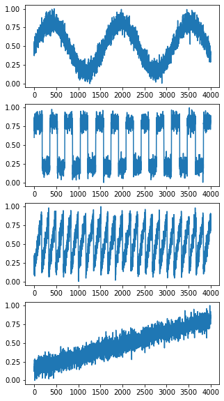
In this first experiment, we use a common example: the decomposition of time series into structural components. The structural components consist in trends, cycles, the seasonality and the irregularity. The trend is a monotone long term signal. The cycle is a signal that affects the observations at random frequencies. Seasonality is a signal that affects the time series at fixed frequency. The exogenous input can be a control variable, an environment factor or some random noise. We generate one seasonal signal, two asynchronous cycles and one trend. These four components are corrupted by additive Gaussian noise (see left plot in Figure 1). The four components are assumed independent.
For the experiment, we mixed the sources with a randomly initialized FBM.


| ICA | FBM + ICA | S-FBM | S-FBM + ICA |
The results clearly show that adding slowness into the FBM model enables to identify the sources. Moreover, we can see that even before the final demixing linear ICA, the slow-FBM gives reasonably good decomposition of the data.
5.3 Audio demixing
We propose a second standard experiment. We propose to recover mixed audio samples. We chose four random instrumental samples and mixed them with a randomly initialized FBM. First of the signal serves as train set, the rest as test set. The four components are assumed independent.


We observe that the decomposition with slow-FBM is noisy, in particular for the sparse signal (number 3 from top). This is due to the little size of the data we used. Adding more data improves the identifiability of true sources (asymptotic result in Khemakhem et al. 2019).
| ICA | FBM + ICA | S-FBM | S-FBM + ICA |
The results again clearly show that adding slowness into the FBM model enables to identify the sources. Moreover, we can see that even before the final demixing linear ICA, the slow-FBM gives reasonably good decomposition of the data.
6 Conclusion and perspectives
In this short paper, we analyzed a simple way to induce identifiability in time series decomposition with flow-based models using slowness. In particular, we used the fact that temporal differentiation is an invertible transform that can be plugged in a chain of normalizing flows. We then related the addition of slowness into FBM to the recent nonlinear blind source separation methods to finally show in simple experiments the advantage of using the slow-FBM instead of FBM for time series decomposition.
Acknowledgments
This work is supported by the company Safran through the CIFRE convention 2017/1317.
References
- Baldi & Pineda (1991) Baldi, P. and Pineda, F. Contrastive learning and neural oscillations. Neural Computation, 3(4):526–545, 1991.
- Blaschke et al. (2007) Blaschke, T., Zito, T., and Wiskott, L. Independent slow feature analysis and nonlinear blind source separation. Neural computation, 19(4):994–1021, 2007.
- Böhmer et al. (2011) Böhmer, W., Grünewälder, S., Nickisch, H., and Obermayer, K. Regularized sparse kernel slow feature analysis. In Joint European Conference on Machine Learning and Knowledge Discovery in Databases, pp. 235–248. Springer, 2011.
- Dinh et al. (2014) Dinh, L., Krueger, D., and Bengio, Y. Nice: Non-linear independent components estimation. arXiv preprint arXiv:1410.8516, 2014.
- Dinh et al. (2016) Dinh, L., Sohl-Dickstein, J., and Bengio, S. Density estimation using real nvp. arXiv preprint arXiv:1605.08803, 2016.
- Du et al. (2019) Du, B., Ru, L., Wu, C., and Zhang, L. Unsupervised deep slow feature analysis for change detection in multi-temporal remote sensing images. IEEE Transactions on Geoscience and Remote Sensing, 57(12):9976–9992, 2019.
- Hyvarinen & Morioka (2016) Hyvarinen, A. and Morioka, H. Unsupervised feature extraction by time-contrastive learning and nonlinear ica. In Advances in Neural Information Processing Systems, pp. 3765–3773, 2016.
- Hyvarinen & Morioka (2017) Hyvarinen, A. and Morioka, H. Nonlinear ica of temporally dependent stationary sources. Proceedings of Machine Learning Research, 2017.
- Hyvärinen & Oja (2000) Hyvärinen, A. and Oja, E. Independent component analysis: algorithms and applications. Neural networks, 13(4-5):411–430, 2000.
- Hyvärinen & Pajunen (1999) Hyvärinen, A. and Pajunen, P. Nonlinear independent component analysis: Existence and uniqueness results. Neural Networks, 12(3):429–439, 1999.
- Hyvärinen et al. (2001) Hyvärinen, A., Karhunen, J., and Oja, E. Methods using time structure. Independent Component Analysis, John Wiley & Sons, Inc, pp. 341–354, 2001.
- Hyvarinen et al. (2019) Hyvarinen, A., Sasaki, H., and Turner, R. Nonlinear ica using auxiliary variables and generalized contrastive learning. In The 22nd International Conference on Artificial Intelligence and Statistics, pp. 859–868, 2019.
- Khemakhem et al. (2019) Khemakhem, I., Kingma, D. P., and Hyvärinen, A. Variational autoencoders and nonlinear ica: A unifying framework. arXiv preprint arXiv:1907.04809, 2019.
- Kingma & Welling (2013) Kingma, D. P. and Welling, M. Auto-encoding variational bayes. arXiv preprint arXiv:1312.6114, 2013.
- Papamakarios et al. (2019) Papamakarios, G., Nalisnick, E., Rezende, D. J., Mohamed, S., and Lakshminarayanan, B. Normalizing flows for probabilistic modeling and inference. arXiv preprint arXiv:1912.02762, 2019.
- Pfau et al. (2018) Pfau, D., Petersen, S., Agarwal, A., Barrett, D. G., and Stachenfeld, K. L. Spectral inference networks: Unifying deep and spectral learning. arXiv preprint arXiv:1806.02215, 2018.
- Rezende & Mohamed (2015) Rezende, D. J. and Mohamed, S. Variational inference with normalizing flows. arXiv preprint arXiv:1505.05770, 2015.
- Schüler et al. (2018) Schüler, M., Hlynsson, H. D., and Wiskott, L. Gradient-based training of slow feature analysis by differentiable approximate whitening. arXiv preprint arXiv:1808.08833, 2018.
- Sorrenson et al. (2020) Sorrenson, P., Rother, C., and Köthe, U. Disentanglement by nonlinear ica with general incompressible-flow networks (gin). International Conference on Learning Representation, 2020.
- Sprekeler et al. (2014) Sprekeler, H., Zito, T., and Wiskott, L. An extension of slow feature analysis for nonlinear blind source separation. The Journal of Machine Learning Research, 15(1):921–947, 2014.
- Tong et al. (1991) Tong, L., Liu, R.-W., Soon, V. C., and Huang, Y.-F. Indeterminacy and identifiability of blind identification. IEEE Transactions on circuits and systems, 38(5):499–509, 1991.
- Tschannen et al. (2018) Tschannen, M., Bachem, O., and Lucic, M. Recent advances in autoencoder-based representation learning. arXiv preprint arXiv:1812.05069, 2018.
- Turner & Sahani (2007) Turner, R. and Sahani, M. A maximum-likelihood interpretation for slow feature analysis. Neural computation, 19(4):1022–1038, 2007.
- Wiskott & Sejnowski (2002) Wiskott, L. and Sejnowski, T. J. Slow feature analysis: Unsupervised learning of invariances. Neural computation, 14(4):715–770, 2002.