跳到论文正文
W Papers独立论文阅读器 arXiv:2007.10178 论文正文 计算阅读时间 · 0%
引用这篇论文根据当前论文元数据生成,正式投稿前建议核对。


License: arXiv.org perpetual non-exclusive license
arXiv:2007.10178v1 [math.NA] 20 Jul 2020

Optimization based model order reduction for stochastic systems

Martin Redmann Thanks: Martin Luther University Halle-Wittenberg, Institute of Mathematics, Theodor-Lieser-Str. 5, 06120 Halle (Saale), Germany, Email: martin.redmann@mathematik.uni-halle.de.    Melina A. Freitag Thanks: Institut für Mathematik, Universität Potsdam, Campus Golm, Karl-Liebknecht-Str. 24-25, 14476 Potsdam, Germany, Email: melina.freitag@uni-potsdam.de
Abstract

In this paper, we bring together the worlds of model order reduction for stochastic linear systems and ℋ2\mathcal{H}_{2}-optimal model order reduction for deterministic systems. In particular, we supplement and complete the theory of error bounds for model order reduction of stochastic differential equations. With these error bounds, we establish a link between the output error for stochastic systems (with additive and multiplicative noise) and modified versions of the ℋ2\mathcal{H}_{2}-norm for both linear and bilinear deterministic systems. When deriving the respective optimality conditions for minimizing the error bounds, we see that model order reduction techniques related to iterative rational Krylov algorithms (IRKA) are very natural and effective methods for reducing the dimension of large-scale stochastic systems with additive and/or multiplicative noise. We apply modified versions of (linear and bilinear) IRKA to stochastic linear systems and show their efficiency in numerical experiments.

Keywords: model order reduction ⋅\cdot stochastic systems ⋅\cdot optimality conditions ⋅\cdot Sylvester equations ⋅\cdot Lévy process

MSC classification: 93A15 ⋅\cdot 93B40 ⋅\cdot 65C30 ⋅\cdot 93E03

1 Introduction

We consider the following linear stochastic systems

d​x​(t)\displaystyle dx(t) =[A​x​(t)+B1​u​(t)]​d​t+f⁡(x⁡(t),d​M​(t)),x⁡(0)=x0,\displaystyle=[Ax(t)+B_{1}u(t)]dt+f(x(t),dM(t)),\quad x(0)=x_{0}, (1a)
y⁡(t)\displaystyle y(t) =C​x​(t),t≥0,\displaystyle=Cx(t),\quad t\geq 0, (1b)

and the function ff represents either additive or multiplicative noise, i.e.,

f⁡(x⁡(t),d​M​(t))={B2​d​M​(t),additive case ∑i=1m2Ni​x​(t−)​d​Mi​(t),multiplicative case,\displaystyle f(x(t),dM(t))=\begin{cases}B_{2}dM(t),&\text{additive case }\\ \sum_{i=1}^{m_{2}}N_{i}x(t-)dM_{i}(t),&\text{multiplicative case},\end{cases}

where x⁡(t−):=lims↑tx⁡(s)x(t-):=\lim_{s\uparrow t}x(s). Above, we assume that A,Ni∈ℝn×nA,N_{i}\in\mathbb{R}^{n\times n}, B1∈ℝn×m1B_{1}\in\mathbb{R}^{n\times m_{1}}, B2∈ℝn×m2B_{2}\in\mathbb{R}^{n\times m_{2}}, and C∈ℝp×nC\in\mathbb{R}^{p\times n} are constant matrices. The vectors x⁡(t)∈ℝnx(t)\in\mathbb{R}^{n}, u⁡(t)∈ℝm1u(t)\in\mathbb{R}^{m_{1}} and y⁡(t)∈ℝpy(t)\in\mathbb{R}^{p} are called state, control input and output vector, respectively. Moreover, let M=(M1,…,Mm2)TM=\left(M_{1},\ldots,M_{m_{2}}\right)^{T} be an ℝm2\mathbb{R}^{m_{2}}-valued square integrable Lévy process with mean zero and covariance matrix K=(ki​j)i,j=1,…,m2K=(k_{ij})_{i,j=1,\ldots,m_{2}}, i.e., 𝔼⁡[M⁡(t)​MT​(t)]=K​t\mathbb{E}[M(t)M^{T}(t)]=Kt for t≥0t\geq 0. Such a matrix exists, see, e.g., [23].

MM and all stochastic process appearing in this paper are defined on a filtered probability space (Ω,ℱ,(ℱt)t≥0,ℙ)\left(\Omega,\mathcal{F},(\mathcal{F}_{t})_{t\geq 0},\mathbb{P}\right)11 1 (ℱt)t≥0(\mathcal{F}_{t})_{t\geq 0} is right continuous and complete.. In addition, MM is (ℱt)t≥0(\mathcal{F}_{t})_{t\geq 0}-adapted and its increments M⁡(t+h)−M⁡(t)M(t+h)-M(t) are independent of ℱt\mathcal{F}_{t} for t,h≥0t,h\geq 0. Throughout this paper, we assume that uu is an (ℱt)t≥0(\mathcal{F}_{t})_{t\geq 0}-adapted control that is square integrable meaning that

‖u‖LT22:=𝔼​∫0T‖u⁡(s)‖2​𝑑s<∞\displaystyle\left\|u\right\|^{2}_{L^{2}_{T}}:=\mathbb{E}\int_{0}^{T}\left\|u(s)\right\|^{2}ds<\infty

for all T>0T>0.

In recent years, model order reduction (MOR) techniques such as balanced truncation (BT) and singular perturbation approximation (SPA), methods well-known and well-understood for deterministic systems [2, 20, 22] have been extended to stochastic systems of the form (1), see, for example [7, 8, 27, 28]. In this paper we discuss optimization based model order reduction techniques for stochastic systems, which will lead naturally to iterative rational Krylov algorithms (IRKA), methods well-known for deterministic systems.

IRKA was introduced in [12] (for systems (1) with f≡0f\equiv 0) and relies on finding a suitable bound (ℋ2\mathcal{H}_{2}-error) for the output error of two systems with the same structure but, as in the context of MOR, one is usually large-scale and the other one is of small order. Subsequently, first order optimality conditions for this ℋ2\mathcal{H}_{2}-bound with respect to the reduced order model (ROM) coefficients were derived. These optimality conditions can be based on system Gramians [15, 29] or they can be equivalently formulated as interpolatory conditions [12, 19] associated to transfer functions of the systems. It was shown in [12] that IRKA fits these conditions. This ℋ2\mathcal{H}_{2}-optimal scheme was extended in the linear deterministic setting to minimizing systems errors in weighted norms [1, 9, 13].

An extension of IRKA to bilinear systems, which relies on the Gramian based optimality conditions shown in [30] was given in [6]. The respective interpolatory optimality conditions in the bilinear case were proved in [11]. However, in contrast to the linear case, bilinear IRKA in [6] was developed without knowing about the link between the bilinear ℋ2\mathcal{H}_{2}-distance and the output error of two bilinear systems. Later this gap was closed in [25] showing that the bilinear ℋ2\mathcal{H}_{2}-error bounds the output error if one involves the exponential of the control energy.

In order to establish IRKA for stochastic systems (1) as an alternative to balancing related MOR, we develop a theory as follows. We prove an output error between two stochastic systems with multiplicative noise and derive the respective first order conditions for optimality in Section 2. The bound in the stochastic case (12) covers the ℋ2\mathcal{H}_{2}-error of two bilinear system as special cases, the same is true for the optimality conditions which generalize the ones in [30]. However, in the stochastic case, in contrast to the bilinear case, the bound does not include the additional factor of the exponential of the control energy. Hence the bound is expected to be much tighter for stochastic system. Based on the optimality conditions for (12) we propose a modified version of bilinear IRKA. Based on the structure of the bound in (12) modified bilinear IRKA appears to be an even more natural method to reduce stochastic systems rather than bilinear systems.

For the case of additive noise, which we consider in Section 3, the first order optimality conditions are merely a special case of the ones for multiplicative noise. As an additional feature we introduce a splitting approach for systems with additive noise in this section, where we split the linear system into two subsystems; one which includes the deterministic part and one the additive noise. We reduce each subsystem independently, which allows for additional flexibility, in case that one of the systems is easier to reduce. Moreover, we consider a one step approach which reduced the deterministic and the noisy part simultaneously. Again, error bounds are provided which naturally lead to (weighted) versions of linear IRKA for each subsystem for the reduction process.

The final Section 4 contains numerical experiments for systems with both multiplicative and additive noise in order to support our theoretical results.

2 Systems with multiplicative noise

We study the multiplicative case first, in which (1) becomes

d​x​(t)\displaystyle dx(t) =[A​x​(t)+B1​u​(t)]​d​t+∑i=1m2Ni​x​(t−)​d​Mi​(t),x⁡(0)=x0,\displaystyle=[Ax(t)+B_{1}u(t)]dt+\sum_{i=1}^{m_{2}}N_{i}x(t-)dM_{i}(t),\quad x(0)=x_{0}, (2a)
y⁡(t)\displaystyle y(t) =C​x​(t),t≥0.\displaystyle=Cx(t),\quad t\geq 0. (2b)

Now, the goal is to find a measure for the distance between (2) and a second system having the same structure but potentially a much smaller dimension. It is given by

d​x^​(t)\displaystyle d\hat{x}(t) =[A^​x^​(t)+B^1​u​(t)]​d​t+∑i=1m2N^i​x^​(t−)​d​Mi​(t),x^​(0)=x^0,\displaystyle=[\hat{A}\hat{x}(t)+{\hat{B}}_{1}u(t)]dt+\sum_{i=1}^{m_{2}}{\hat{N}}_{i}\hat{x}(t-)dM_{i}(t),\quad\hat{x}(0)={\hat{x}}_{0}, (3a)
y^​(t)\displaystyle\hat{y}(t) =C^​x^​(t),t≥0,\displaystyle=\hat{C}\hat{x}(t),\quad t\geq 0, (3b)

where x^​(t)∈ℝr\hat{x}(t)\in\mathbb{R}^{r}, with r≪nr\ll n and A^\hat{A}, B^1{\hat{B}}_{1}, C^\hat{C}, N^i{\hat{N}}_{i}, i=1,…,m2i=1,\ldots,m_{2} of appropriate dimension. In order to find a distance between the above systems, a stability assumption and the fundamental solution to both systems are needed. Some results (in particular the one on the optimality for the error between two systems) obtained for systems with multiplicative noise can be transferred to the case with additive noise as we will see later.

2.1 Fundamental solutions and stability

We introduce the fundamental solution Φ\Phi to (2a). It is defined as the ℝn×n\mathbb{R}^{n\times n}-valued solution to

Φ⁡(t,s)=I+∫stA​Φ​(τ,s)​𝑑τ+∑i=1m2∫stNi​Φ​(τ−,s)​d​Mi​(τ),t≥s.\displaystyle\Phi(t,s)=I+\int_{s}^{t}A\Phi(\tau,s)d\tau+\sum_{i=1}^{m_{2}}\int_{s}^{t}N_{i}\Phi(\tau-,s)dM_{i}(\tau),\quad t\geq s. (4)

This operator maps the initial condition x0x_{0} to the solution of the homogeneous state equation with initial time s≥0s\geq 0. We additionally define Φ⁡(t):=Φ⁡(t,0)\Phi(t):=\Phi(t,0). Note, that Φ\Phi also includes the fundamental solution of the additive noise scenario which we will use later. It is obtained by setting N1=…=Nm2=0N_{1}=\ldots=N_{m_{2}}=0 in (4), so that Φ⁡(t,s)=eA⁡(t−s)\Phi(t,s)=\operatorname{e}^{A(t-s)}. We make a stability assumption on the fundamental solution which we need to produce well-defined system norms (and distances).

Assumption 1.

The fundamental solution Φ\Phi is mean square asymptotically stable, i.e., there is a constant c>0c>0 such that

𝔼​‖Φ⁡(t)‖2≲e−c​t⇔λ⁡(I⊗A+A⊗I+∑i,j=1m2Ni⊗Nj​ki​j)⊂ℂ−,\displaystyle\mathbb{E}\left\|\Phi(t)\right\|^{2}\lesssim\operatorname{e}^{-ct}\Leftrightarrow\lambda\left(I\otimes A+A\otimes I+\sum_{i,j=1}^{m_{2}}N_{i}\otimes N_{j}k_{ij}\right)\subset\mathbb{C}_{-}, (5)

where λ⁡(⋅)\lambda(\cdot) denotes the spectrum of a matrix. We refer to [24] for the equivalence in (5), or to [17] for the same result in case of standard Wiener noise.

Note that, with additive noise (Ni=0,∀iN_{i}=0,\forall i in (4)), condition (5) simplifies to

‖eA​t‖2≲e−c​t⇔λ⁡(A)⊂ℂ−.\displaystyle\left\|\operatorname{e}^{At}\right\|^{2}\lesssim\operatorname{e}^{-ct}\Leftrightarrow\lambda\left(A\right)\subset\mathbb{C}_{-}. (6)

The fundamental solution is a vital tool to compute error bounds between two different stochastic systems. The key result to establish these bounds is the following lemma which is a generalization of [8, Proposition 4.4].

Lemma 2.1.

Let Φ\Phi be the fundamental solution of the stochastic differential equation with coefficients A,Ni∈ℝn×nA,N_{i}\in\mathbb{R}^{n\times n} defined in (4) and let Φ^\hat{\Phi} be the one of the same system, where A,NiA,N_{i} are replaced by A^,N^i∈ℝr×r\hat{A},\hat{N}_{i}\in\mathbb{R}^{r\times r}. Moreover, suppose that LL and L^\hat{L} are matrices of suitable dimension. Then, the ℝn×r\mathbb{R}^{n\times r}-valued function 𝔼⁡[Φ⁡(t,s)​L​L^T​Φ^T​(t,s)]\mathbb{E}\left[\Phi(t,s)L{\hat{L}}^{T}\hat{\Phi}^{T}(t,s)\right], t≥st\geq s, satisfies

X˙​(t)=X⁡(t)​A^T+A​X​(t)+∑i,j=1m2Ni​X​(t)​N^jT​ki​j,X⁡(s)=L​L^T.\displaystyle\dot{X}(t)=X(t){\hat{A}}^{T}+AX(t)+\sum_{i,j=1}^{m_{2}}N_{i}X(t){\hat{N}}_{j}^{T}\;k_{ij},\quad X(s)=L{\hat{L}}^{T}. (7)
Proof.

See Appendix B. ∎

Lemma 2.1 yields

𝔼⁡[Φ⁡(t,s)​L​L^T​Φ^T​(t,s)]=𝔼⁡[Φ⁡(t−s)​L​L^T​Φ^T​(t−s)]\displaystyle\mathbb{E}\left[\Phi(t,s)L{\hat{L}}^{T}\hat{\Phi}^{T}(t,s)\right]=\mathbb{E}\left[\Phi(t-s)L{\hat{L}}^{T}\hat{\Phi}^{T}(t-s)\right] (8)

for all t≥s≥0t\geq s\geq 0, since both expressions solve (7).

2.2 The stochastic analogue to ℋ2\mathcal{H}_{2}-norms

For deterministic linear systems (system (1) without noise), a transfer function GG can be interpreted as an input-output map in the frequency domain, i.e., y~=G​u~\tilde{y}=G\tilde{u}, where u~\tilde{u} and y~\tilde{y} are the Laplace transforms of the input and the output, receptively. A norm associated with this transfer function can subsequently be defined that provides a bound for the norm of the output. This can, e.g., be the ℋ2\mathcal{H}_{2}-norm of GG which in the linear deterministic case is given by

‖G‖ℋ22:=12​π​∫−∞∞‖G⁡(i​w)‖F2​𝑑w,\displaystyle\left\|G\right\|^{2}_{\mathcal{H}_{2}}:=\frac{1}{2\pi}\int_{-\infty}^{\infty}\left\|G(\mathrm{i}w)\right\|^{2}_{F}dw,

where ‖⋅‖F\left\|\cdot\right\|_{F} denotes the Frobenius norm and i\mathrm{i} the imaginary unit. However, there are no transfer functions in the stochastic case but we can still define a norm that is analogue to the ℋ2\mathcal{H}_{2}-norm. To do so, we use a connection known in the linear deterministic case. There, the ℋ2\mathcal{H}_{2}-norm of a transfer function coincides with the L2L^{2}-norm of the impulse response of the system, that is,

‖G‖ℋ22=∫0∞‖C​eA​s​B1‖F2​𝑑s,\left\|G\right\|^{2}_{\mathcal{H}_{2}}=\int_{0}^{\infty}\left\|Ce^{As}B_{1}\right\|^{2}_{F}ds,

see [2]. A generalized impulse response exists in the stochastic setting (2) and is given by H⁡(t):=C​Φ​(t)​B1H(t):=C\Phi(t)B_{1}, where Φ\Phi is the fundamental solution defined in (4). We introduce a space ℒ2​(𝒲)\mathcal{L}^{2}(\mathcal{W}) of matrix-valued and (ℱt)t≥0(\mathcal{F}_{t})_{t\geq 0}-adapted stochastic processes YY of appropriate dimension with

‖Y‖ℒ2​(𝒲)2:=𝔼​∫0∞‖Y⁡(s)​𝒲‖F2​𝑑s<∞,\displaystyle\left\|Y\right\|^{2}_{\mathcal{L}^{2}(\mathcal{W})}:=\mathbb{E}\int_{0}^{\infty}\left\|Y(s)\mathcal{W}\right\|^{2}_{F}ds<\infty,

and 𝒲\mathcal{W} is a regular m1×m1m_{1}\times m_{1} matrix that can be seen as a weight (in the simplest case the identity matrix) and will be specified later. Now, the stochastic analogue to the (weighted) ℋ2\mathcal{H}_{2}-norm for system (2) is

‖H‖ℒ2​(𝒲)=(𝔼​∫0∞‖C​Φ​(s)​B1​𝒲‖F2​𝑑s)12,\displaystyle\left\|H\right\|_{\mathcal{L}^{2}(\mathcal{W})}=\left(\mathbb{E}\int_{0}^{\infty}\left\|C\Phi(s)B_{1}\mathcal{W}\right\|^{2}_{F}ds\right)^{\frac{1}{2}},

which is finite due to Assumption 1. Let Φ^\hat{\Phi} denote the fundamental solution to the reduced system (3) and H^​(t):=C^​Φ^​(t)​B^1\hat{H}(t):=\hat{C}\hat{\Phi}(t)\hat{B}_{1} its impulse response. Then, we can specify the distance between HH and H^\hat{H}. A Gramian based representation is stated in the next theorem.

Theorem 2.2.

Let HH and H^\hat{H} be the impulse responses of systems (2) and (3), respectively. Moreover, suppose that Assumption 1 holds for (2) and (3). Then, we have

‖H−H^‖ℒ2​(𝒲)2=‖C​Φ​B1−C^​Φ^​B^1‖ℒ2​(𝒲)2=tr⁡(C​P​CT)+tr⁡(C^​P^​C^T)−2​tr⁡(C​P2​C^T),\displaystyle\left\|H-\hat{H}\right\|_{\mathcal{L}^{2}(\mathcal{W})}^{2}=\left\|C\Phi B_{1}-\hat{C}\hat{\Phi}\hat{B}_{1}\right\|_{\mathcal{L}^{2}(\mathcal{W})}^{2}=\operatorname{tr}(CPC^{T})+\operatorname{tr}(\hat{C}\hat{P}{\hat{C}}^{T})-2\operatorname{tr}(CP_{2}{\hat{C}}^{T}),

where the matrices P,P^P,\hat{P} and P2P_{2} are the solutions to

A​P+P​AT+∑i,j=1m2Ni​P​NjT​ki​j\displaystyle AP+PA^{T}+\sum_{i,j=1}^{m_{2}}N_{i}PN_{j}^{T}k_{ij} =−B1​𝒲​(B1​𝒲)T,\displaystyle=-B_{1}\mathcal{W}(B_{1}\mathcal{W})^{T}, (9)
A^​P^+P^​A^T+∑i,j=1m2N^i​P^​N^jT​ki​j\displaystyle\hat{A}\hat{P}+\hat{P}{\hat{A}}^{T}+\sum_{i,j=1}^{m_{2}}\hat{N}_{i}\hat{P}{\hat{N}}_{j}^{T}k_{ij} =−B^1​𝒲​(B^1​𝒲)T\displaystyle=-\hat{B}_{1}\mathcal{W}(\hat{B}_{1}\mathcal{W})^{T} (10)
A​P2+P2​A^T+∑i,j=1m2Ni​P2​N^jT​ki​j\displaystyle AP_{2}+P_{2}{\hat{A}}^{T}+\sum_{i,j=1}^{m_{2}}N_{i}P_{2}{\hat{N}}_{j}^{T}k_{ij} =−B1​𝒲​(B^1​𝒲)T.\displaystyle=-B_{1}\mathcal{W}(\hat{B}_{1}\mathcal{W})^{T}. (11)
Proof.

We have that

‖H−H^‖ℒ2​(𝒲)2=\displaystyle\left\|H-\hat{H}\right\|_{\mathcal{L}^{2}(\mathcal{W})}^{2}=\; 𝔼​∫0∞‖(C​Φ​(s)​B1−C^​Φ^​(s)​B^1)​𝒲‖F2​𝑑s\displaystyle\mathbb{E}\int_{0}^{\infty}\left\|(C\Phi(s)B_{1}-\hat{C}\hat{\Phi}(s)\hat{B}_{1})\mathcal{W}\right\|^{2}_{F}ds
=\displaystyle=\; 𝔼​∫0∞tr⁡(C​Φ​(s)​(B1​𝒲)​(B1​𝒲)T​ΦT​(s)​CT)​𝑑s\displaystyle\mathbb{E}\int_{0}^{\infty}\operatorname{tr}\left(C\Phi(s)(B_{1}\mathcal{W})(B_{1}\mathcal{W})^{T}\Phi^{T}(s)C^{T}\right)ds
+𝔼∫0∞tr(C^Φ^(s)(B^1𝒲)(B^1𝒲)TΦ^T(s)C^T)ds\displaystyle+\mathbb{E}\int_{0}^{\infty}\operatorname{tr}\left(\hat{C}\hat{\Phi}(s)(\hat{B}_{1}\mathcal{W})(\hat{B}_{1}\mathcal{W})^{T}\hat{\Phi}^{T}(s)\hat{C}^{T}\right)ds
−2𝔼∫0∞tr(CΦ(s)(B1𝒲)(B^1𝒲)TΦ^T(s)C^T)ds\displaystyle-2\mathbb{E}\int_{0}^{\infty}\operatorname{tr}\left(C\Phi(s)(B_{1}\mathcal{W})(\hat{B}_{1}\mathcal{W})^{T}\hat{\Phi}^{T}(s)\hat{C}^{T}\right)ds

using the properties of the Frobenius norm. Due to the linearity of the trace and the integral, we find

‖H−H^‖ℒ2​(𝒲)2=tr⁡(C​P​CT)+tr⁡(C^​P^​C^T)−2​tr⁡(C​P2​C^T),\displaystyle\left\|H-\hat{H}\right\|_{\mathcal{L}^{2}(\mathcal{W})}^{2}=\operatorname{tr}(CPC^{T})+\operatorname{tr}(\hat{C}\hat{P}{\hat{C}}^{T})-2\operatorname{tr}(CP_{2}{\hat{C}}^{T}),

where we set

P:=\displaystyle P:= ∫0∞𝔼⁡[Φ⁡(s)​(B1​𝒲)​(B1​𝒲)T​ΦT​(s)]​𝑑s,P^:=∫0∞𝔼⁡[Φ^​(s)​(B^1​𝒲)​(B^1​𝒲)T​Φ^T​(s)]​𝑑s,\displaystyle\int_{0}^{\infty}\mathbb{E}\left[\Phi(s)(B_{1}\mathcal{W})(B_{1}\mathcal{W})^{T}\Phi^{T}(s)\right]ds,\quad\hat{P}:=\int_{0}^{\infty}\mathbb{E}\left[\hat{\Phi}(s)(\hat{B}_{1}\mathcal{W})(\hat{B}_{1}\mathcal{W})^{T}\hat{\Phi}^{T}(s)\right]ds,
P2:=∫0∞𝔼⁡[Φ⁡(s)​(B1​𝒲)​(B^1​𝒲)T​Φ^T​(s)]​𝑑s.\displaystyle\quad\quad\quad\quad\quad\quad\quad P_{2}:=\int_{0}^{\infty}\mathbb{E}\left[\Phi(s)(B_{1}\mathcal{W})(\hat{B}_{1}\mathcal{W})^{T}\hat{\Phi}^{T}(s)\right]ds.

Notice that P,P^P,\hat{P} and P2P_{2} exist due to Assumption 1 for both systems. Now, the function t↦X⁡(t):=𝔼⁡[Φ⁡(t)​(B1​𝒲)​(B^1​𝒲)T​Φ^T​(t)]t\mapsto X(t):=\mathbb{E}\left[\Phi(t)(B_{1}\mathcal{W})(\hat{B}_{1}\mathcal{W})^{T}\hat{\Phi}^{T}(t)\right] solves (7) in Lemma 2.1 with s=0s=0 and L^=B^1​𝒲\hat{L}=\hat{B}_{1}\mathcal{W}, L=B1​𝒲L=B_{1}\mathcal{W}. Integrating (7) over [0,v][0,v] yields

X⁡(v)−(B1​𝒲)​(B^1​𝒲)T=∫0vX⁡(t)​𝑑t​A^T+A​∫0vX⁡(t)​𝑑t+∑i,j=1m2Ni​∫0vX⁡(t)​𝑑t​N^jT​ki​j.\displaystyle X(v)-(B_{1}\mathcal{W})(\hat{B}_{1}\mathcal{W})^{T}=\int_{0}^{v}X(t)dt{\hat{A}}^{T}+A\int_{0}^{v}X(t)dt+\sum_{i,j=1}^{m_{2}}N_{i}\int_{0}^{v}X(t)dt{\hat{N}}_{j}^{T}\;k_{ij}.

Taking the limit of v→∞v\rightarrow\infty above and taking into account that limv→∞X⁡(v)=0\lim_{v\rightarrow\infty}X(v)=0 by assumption, we obtain that P2P_{2} solves (11). With the same arguments setting Φ=Φ^\Phi=\hat{\Phi} and B1=B^1B_{1}=\hat{B}_{1} and vice versa, we see that PP and P^\hat{P} satisfy (9) and (10), respectively. ∎

If m1=m2m_{1}=m_{2} and if we replace the noise in (2a) and (3a) by the components uiu_{i} of the control vector uu, i.e., d​Mi​(t)dM_{i}(t) is replaced by ui​(t)​d​tu_{i}(t)dt, then these systems are so-called (deterministic) bilinear systems. Let us denote these resulting bilinear systems by Σb​i​l\Sigma_{bil} and Σ^b​i​l\hat{\Sigma}_{bil} for the full and reduced system, respectively. Then, an ℋ2\mathcal{H}_{2}-norm can be introduced for the bilinear case, too. We refer to [30] for more details. In [30] a Gramian based representation for ‖Σb​i​l−Σ^b​i​l‖ℋ2\left\|\Sigma_{bil}-\hat{\Sigma}_{bil}\right\|_{\mathcal{H}_{2}} is given. Interestingly, this distance coincides with the one in Theorem 2.2 if the noise and the input dimension coincide (m1=m2m_{1}=m_{2}), and the covariance and weight matrices are the identity (K=(ki​j)=IK=(k_{ij})=I and 𝒲=I\mathcal{W}=I). Consequently, a special case of ‖H−H^‖ℒ2​(𝒲)\left\|H-\hat{H}\right\|_{\mathcal{L}^{2}(\mathcal{W})} yields a stochastic time-domain representation for the metric induced by the ℋ2\mathcal{H}_{2}-norm for bilinear systems, e.g., if MM is an m1m_{1}-dimensional standard Wiener process. We refer to [25] for further connections between bilinear and stochastic linear systems. The next proposition deals with the distance between the outputs yy and y^\hat{y}, defined in (2b) and (3b), and the above stochastic ℋ2\mathcal{H}_{2}-distance ‖H−H^‖ℒ2​(𝒲)\left\|H-\hat{H}\right\|_{\mathcal{L}^{2}(\mathcal{W})} when 𝒲=I\mathcal{W}=I.

Proposition 2.3.

Let yy and y^\hat{y} be the outputs of systems (2) and (3) with x0=0x_{0}=0, x^0=0\hat{x}_{0}=0 and let H=C​Φ​(⋅)​B1H=C\Phi(\cdot)B_{1}, H^=C^​Φ^​(⋅)​B^1\hat{H}=\hat{C}\hat{\Phi}(\cdot)\hat{B}_{1} the impulse responses of these systems. Then, for T>0T>0, we have

supt∈[0,T]𝔼⁡‖y⁡(t)−y^​(t)‖≤‖H−H^‖ℒ2​(I)​‖u‖LT2.\displaystyle\sup_{t\in[0,T]}\mathbb{E}\left\|y(t)-\hat{y}(t)\right\|\leq\left\|H-\hat{H}\right\|_{\mathcal{L}^{2}(I)}\left\|u\right\|_{L^{2}_{T}}. (12)
Proof.

We find a solution representation for (2a) by

x⁡(t)=Φ⁡(t)​x0+∫0tΦ⁡(t,s)​B1​u​(s)​𝑑s,\displaystyle x(t)=\Phi(t)x_{0}+\int_{0}^{t}\Phi(t,s)B_{1}u(s)ds,

where Φ⁡(t,s)=Φ⁡(t)​Φ−1​(s)\Phi(t,s)=\Phi(t)\Phi^{-1}(s) satisfies (4). This is obtained by applying Ito’s formula in (28) to Φ⁡(t)​g​(t)\Phi(t)g(t) with g⁡(t):=x0+∫0tΦ−1​(s)​B1​u​(s)​𝑑sg(t):=x_{0}+\int_{0}^{t}\Phi^{-1}(s)B_{1}u(s)ds using that Φ\Phi and gg are semimartingales, see Appendix A. Since gg is continuous and has a martingale part zero, (28) simply becomes the standard product rule due to (29) and one can show that Φ⁡(t)​g​(t)\Phi(t)g(t) is the solution to (2a). We proceed with the arguments used in [8]. The representations for the reduced and the full state with zero initial states yield

𝔼​‖y​(t)−y^​(t)‖\displaystyle\mathbb{E}\left\|y(t)-\hat{y}(t)\right\| ≤𝔼​∫0t‖(C​Φ​(t,s)​B1−C^​Φ^​(t,s)​B^1)​u​(s)‖​𝑑s\displaystyle\leq\mathbb{E}\int_{0}^{t}\left\|\left(C\Phi(t,s)B_{1}-\hat{C}\hat{\Phi}(t,s)\hat{B}_{1}\right)u(s)\right\|ds
≤𝔼​∫0t‖C​Φ​(t,s)​B1−C^​Φ^​(t,s)​B^1‖F​‖u⁡(s)‖​𝑑s.\displaystyle\leq\mathbb{E}\int_{0}^{t}\left\|C\Phi(t,s)B_{1}-\hat{C}\hat{\Phi}(t,s)\hat{B}_{1}\right\|_{F}\left\|u(s)\right\|ds.

We apply the Cauchy-Schwarz inequality and obtain

𝔼⁡‖y⁡(t)−y^​(t)‖≤(𝔼​∫0t‖C​Φ​(t,s)​B1−C^​Φ^​(t,s)​B^1‖F2​𝑑s)12​‖u‖Lt2.\displaystyle\mathbb{E}\left\|y(t)-\hat{y}(t)\right\|\leq\left(\mathbb{E}\int_{0}^{t}\left\|C\Phi(t,s)B_{1}-\hat{C}\hat{\Phi}(t,s)\hat{B}_{1}\right\|_{F}^{2}ds\right)^{\frac{1}{2}}\left\|u\right\|_{L^{2}_{t}}.

Now, 𝔼⁡[Φ⁡(t,s)​B1​B^1​Φ^​(t,s)]=𝔼⁡[Φ⁡(t−s)​B1​B^1​Φ^​(t−s)]\mathbb{E}[\Phi(t,s)B_{1}\hat{B}_{1}\hat{\Phi}(t,s)]=\mathbb{E}[\Phi(t-s)B_{1}\hat{B}_{1}\hat{\Phi}(t-s)] due to (8). Since the same property holds when considering B1=B^1B_{1}=\hat{B}_{1} and Φ=Φ^\Phi=\hat{\Phi}, we find

𝔼​‖y​(t)−y^​(t)‖\displaystyle\mathbb{E}\left\|y(t)-\hat{y}(t)\right\| ≤(𝔼​∫0t‖C​Φ​(t−s)​B1−C^​Φ^​(t−s)​B^1‖F2​𝑑s)12​‖u‖Lt2\displaystyle\leq\left(\mathbb{E}\int_{0}^{t}\left\|C\Phi(t-s)B_{1}-\hat{C}\hat{\Phi}(t-s)\hat{B}_{1}\right\|_{F}^{2}ds\right)^{\frac{1}{2}}\left\|u\right\|_{L^{2}_{t}}
=(𝔼​∫0t‖C​Φ​(s)​B1−C^​Φ^​(s)​B^1‖F2​𝑑s)12​‖u‖Lt2.\displaystyle=\left(\mathbb{E}\int_{0}^{t}\left\|C\Phi(s)B_{1}-\hat{C}\hat{\Phi}(s)\hat{B}_{1}\right\|_{F}^{2}ds\right)^{\frac{1}{2}}\left\|u\right\|_{L^{2}_{t}}.

Taking the supremum on both sides and the upper bound of the integral to infinity implies the result. ∎

If 𝔼​∫0∞‖u⁡(s)‖2​𝑑s<∞\mathbb{E}\int_{0}^{\infty}\left\|u(s)\right\|^{2}ds<\infty, then we can replace [0,T][0,T] by [0,∞)[0,\infty) in Proposition 2.3. The above result shows that one can expect a good approximation of (2) by (3) if matrices A^,N^i,B^1,C^\hat{A},\hat{N}_{i},\hat{B}_{1},\hat{C} are chosen such that ‖H−H^‖ℒ2​(I)\left\|H-\hat{H}\right\|_{\mathcal{L}^{2}(I)} is minimal. As mentioned above, ‖H−H^‖ℒ2​(I)\left\|H-\hat{H}\right\|_{\mathcal{L}^{2}(I)} coincides with the ℋ2\mathcal{H}_{2}-distance of the corresponding bilinear systems in special cases. In the bilinear case, MOR techniques have been considered that minimize the ℋ2\mathcal{H}_{2}-error of two systems, e.g., bilinear IRKA [6]. Below, we construct related (ℒ2​(𝒲){\mathcal{L}^{2}(\mathcal{W})}-optimal) algorithms which are very natural for stochastic systems due to Proposition 2.3, where 𝒲=I\mathcal{W}=I. Note that for bilinear systems, the above proposition can only be shown if the right hand side is additionally multiplied by exp⁡{0.5​‖u‖LT22}\exp\left\{0.5\left\|u\right\|^{2}_{L^{2}_{T}}\right\}. This is a very recent result proved in [25]. Therefore, considering IRKA type methods for stochastic systems seems even more natural than in the bilinear case in terms of the expected output error.

Remark 1.

The error bound in Proposition 2.3 was shown for the special case of uncorrelated noise processes MiM_{i} in [8] and used to determine an error bound for balanced truncation. The bound in [8] was also the basis for the proof of an error bound for another balancing related method in [27].

2.3 Conditions for ℒ2​(𝒲)\mathcal{L}^{2}(\mathcal{W})-optimality and model order reduction in the multiplicative case

Motivated by Proposition 2.3, we locally minimize ‖H−H^‖ℒ2​(𝒲)\left\|H-\hat{H}\right\|_{\mathcal{L}^{2}(\mathcal{W})} with respect to the coefficients of the reduced systems (3) using the representation in Theorem 2.2. In particular, we find necessary conditions for optimality for the expression

ℰ⁡(A^,N^i,B^1,C^):=tr⁡(C^​P^​C^T)−2​tr⁡(C​P2​C^T),\displaystyle\mathcal{E}(\hat{A},\hat{N}_{i},\hat{B}_{1},\hat{C}):=\operatorname{tr}(\hat{C}\hat{P}{\hat{C}}^{T})-2\operatorname{tr}(CP_{2}{\hat{C}}^{T}),

with P^\hat{P} and P2P_{2} solving (10) and (11), respectively.

Theorem 2.4.

Consider the system (2) with impulse response HH. Let the reduced system (3) with impulse response H^\hat{H} be optimal with respect to ℒ2​(𝒲)\mathcal{L}^{2}(\mathcal{W}), i.e., the matrices A^,N^i,B^1,C^\hat{A},\hat{N}_{i},\hat{B}_{1},\hat{C} locally minimize the error ‖H−H^‖ℒ2​(𝒲)\left\|H-\hat{H}\right\|_{\mathcal{L}^{2}(\mathcal{W})}. Then, it holds that

(a)\displaystyle(a) C^​P^=C​P2,(b)Q^​P^=Q2​P2,\displaystyle\hat{C}\hat{P}=CP_{2},\quad(b)\quad\hat{Q}\hat{P}=Q_{2}P_{2}, (13)
(c)\displaystyle(c) Q^(∑j=1m2N^jki​j)P^=Q2(∑j=1m2Njki​j)P2,i=1,…,m2,\displaystyle\hat{Q}\left(\sum_{j=1}^{m_{2}}\hat{N}_{j}k_{ij}\right)\hat{P}=Q_{2}\left(\sum_{j=1}^{m_{2}}N_{j}k_{ij}\right)P_{2},\quad i=1,\ldots,m_{2},
(d)\displaystyle(d) Q^​B^1​𝒲​𝒲T=Q2​B1​𝒲​𝒲T,\displaystyle\hat{Q}\hat{B}_{1}\mathcal{W}\mathcal{W}^{T}=Q_{2}B_{1}\mathcal{W}\mathcal{W}^{T},

where P^,P2\hat{P},P_{2} are the solutions to (10), (11) and Q^,Q2\hat{Q},Q_{2} satisfy

A^T​Q^+Q^​A^+∑i,j=1m2N^iT​Q^​N^j​ki​j\displaystyle\hat{A}^{T}\hat{Q}+\hat{Q}\hat{A}+\sum_{i,j=1}^{m_{2}}\hat{N}_{i}^{T}\hat{Q}\hat{N}_{j}k_{ij} =−C^T​C^,\displaystyle=-\hat{C}^{T}\hat{C}, (14)
A^T​Q2+Q2​A+∑i,j=1m2N^iT​Q2​Nj​ki​j\displaystyle\hat{A}^{T}Q_{2}+Q_{2}A+\sum_{i,j=1}^{m_{2}}\hat{N}_{i}^{T}Q_{2}N_{j}k_{ij} =−C^T​C.\displaystyle=-\hat{C}^{T}C. (15)
Proof.

If system (3) is optimal with respect to the ℒ2​(𝒲)\mathcal{L}^{2}(\mathcal{W})-norm, then we have

∂zℰ=0⟺∂ztr⁡(C^​P^​C^T)=2​∂ztr⁡(C​P2​C^T),\displaystyle\partial_{z}\mathcal{E}=0\Longleftrightarrow\partial_{z}\operatorname{tr}(\hat{C}\hat{P}{\hat{C}}^{T})=2\partial_{z}\operatorname{tr}(CP_{2}{\hat{C}}^{T}), (16)

where z∈{a^k​m,n^k​m(l),b^k​q,c^ℓ​k}z\in\{\hat{a}_{km},\hat{n}^{(l)}_{km},\hat{b}_{kq},\hat{c}_{\ell k}\}, where A^=(a^k​m)\hat{A}=(\hat{a}_{km}), N^l=(n^k​m(l))\hat{N}_{l}=(\hat{n}^{(l)}_{km}), B^1=(b^k​q)\hat{B}_{1}=(\hat{b}_{kq}) and C^=(c^ℓ​k)\hat{C}=(\hat{c}_{\ell k}). Below, eke_{k} denotes the kkth unit vector of suitable dimension. For z=c^ℓ​kz=\hat{c}_{\ell k}, (16) becomes

tr⁡(eℓ​ekT​P^​C^T+C^​P^​ek​eℓT)=2​tr⁡(C​P2​ek​eℓT).\displaystyle\operatorname{tr}(e_{\ell}e_{k}^{T}\hat{P}{\hat{C}}^{T}+{\hat{C}}\hat{P}e_{k}e_{\ell}^{T})=2\operatorname{tr}(CP_{2}e_{k}e_{\ell}^{T}).

Using the properties of the trace and P^T=P^{\hat{P}}^{T}=\hat{P}, this is equivalent to

eℓT​C^​P^​ek=eℓT​C​P2​eke_{\ell}^{T}{\hat{C}}\hat{P}e_{k}=e_{\ell}^{T}CP_{2}e_{k}

for all ℓ=1,…​p\ell=1,\ldots p and k=1,…,rk=1,\ldots,r. This results in equality (a): C^​P^=C​P2\hat{C}\hat{P}=CP_{2}. For z=a^k​m,n^k​m(l),b^k​qz=\hat{a}_{km},\hat{n}^{(l)}_{km},\hat{b}_{kq}, (16) becomes

tr⁡((∂zP^)​C^T​C^)=2​tr⁡((∂zP2)​C^T​C),\displaystyle\operatorname{tr}\left((\partial_{z}\hat{P}){\hat{C}}^{T}\hat{C}\right)=2\operatorname{tr}\left((\partial_{z}P_{2}){\hat{C}}^{T}C\right),

which is equivalent to

tr⁡((∂zP^)​(A^T​Q^+Q^​A^+∑i,j=1m2N^iT​Q^​N^j​ki​j))\displaystyle\operatorname{tr}\left((\partial_{z}\hat{P})(\hat{A}^{T}\hat{Q}+\hat{Q}\hat{A}+\sum_{i,j=1}^{m_{2}}\hat{N}_{i}^{T}\hat{Q}\hat{N}_{j}k_{ij})\right)
=2​tr⁡((∂zP2)​(A^T​Q2+Q2​A+∑i,j=1m2N^iT​Q2​Nj​ki​j))\displaystyle=2\operatorname{tr}\left((\partial_{z}P_{2})(\hat{A}^{T}Q_{2}+Q_{2}A+\sum_{i,j=1}^{m_{2}}\hat{N}_{i}^{T}Q_{2}N_{j}k_{ij})\right)

using the equations for Q^\hat{Q} and Q2Q_{2}. Again, by properties of the trace, the above can be reformulated as

\displaystyle tr⁡((A^​(∂zP^)+(∂zP^)​A^T+∑i,j=1m2N^i​(∂zP^)​N^jT​ki​j)​Q^)\displaystyle\operatorname{tr}\left(\left(\hat{A}(\partial_{z}\hat{P})+(\partial_{z}\hat{P})\hat{A}^{T}+\sum_{i,j=1}^{m_{2}}\hat{N}_{i}(\partial_{z}\hat{P})\hat{N}_{j}^{T}k_{ij}\right)\hat{Q}\right) (17)
=2​tr⁡((A⁡(∂zP2)+(∂zP2)​A^T+∑i,j=1m2Ni​(∂zP2)​N^jT​ki​j)​Q2),\displaystyle=2\operatorname{tr}\left(\left(A(\partial_{z}P_{2})+(\partial_{z}P_{2})\hat{A}^{T}+\sum_{i,j=1}^{m_{2}}N_{i}(\partial_{z}P_{2})\hat{N}_{j}^{T}k_{ij}\right)Q_{2}\right),

taking into account that the covariance matrix K=(ki​j)K=(k_{ij}) is symmetric. We now derive equations for ∂zP^\partial_{z}\hat{P} and ∂zP2\partial_{z}P_{2} for each case. Applying ∂a^k​m\partial_{\hat{a}_{km}} to (10) and (11), we obtain

ek​emT​P^+A^​(∂a^k​mP^)+(∂a^k​mP^)​A^T+P^​em​ekT+∑i,j=1m2N^i​(∂a^k​mP^)​N^jT​ki​j\displaystyle e_{k}e_{m}^{T}\hat{P}+\hat{A}(\partial_{\hat{a}_{km}}\hat{P})+(\partial_{\hat{a}_{km}}\hat{P}){\hat{A}}^{T}+\hat{P}e_{m}e_{k}^{T}+\sum_{i,j=1}^{m_{2}}\hat{N}_{i}(\partial_{\hat{a}_{km}}\hat{P}){\hat{N}}_{j}^{T}k_{ij} =0,\displaystyle=0,
A⁡(∂a^k​mP2)+(∂a^k​mP2)​A^T+P2​em​ekT+∑i,j=1m2Ni​(∂a^k​mP2)​N^jT​ki​j\displaystyle A(\partial_{\hat{a}_{km}}P_{2})+(\partial_{\hat{a}_{km}}P_{2}){\hat{A}}^{T}+P_{2}e_{m}e_{k}^{T}+\sum_{i,j=1}^{m_{2}}N_{i}(\partial_{\hat{a}_{km}}P_{2}){\hat{N}}_{j}^{T}k_{ij} =0.\displaystyle=0.

Inserting this into (17), and using symmetry of Q^\hat{Q} and P^\hat{P} leads to

tr⁡((ek​emT​P^+P^​em​ekT)​Q^)=2​tr⁡((P2​em​ekT)​Q2)⇔ekT​Q^​P^​em=ekT​Q2​P2​em\displaystyle\operatorname{tr}\left((e_{k}e_{m}^{T}\hat{P}+\hat{P}e_{m}e_{k}^{T})\hat{Q}\right)=2\operatorname{tr}\left((P_{2}e_{m}e_{k}^{T})Q_{2}\right)\Leftrightarrow e_{k}^{T}\hat{Q}\hat{P}e_{m}=e_{k}^{T}Q_{2}P_{2}e_{m}

for all k,m=1,…,rk,m=1,\ldots,r which yields Q^​P^=Q2​P2\hat{Q}\hat{P}=Q_{2}P_{2}, i.e. equality (b). We now define Ψ^iT:=∑j=1m2N^jT​ki​j\hat{\Psi}_{i}^{T}:=\sum_{j=1}^{m_{2}}{\hat{N}}_{j}^{T}k_{ij} and observe that ∂n^k​m(l)Ψ^iT=em​ekT​ki​l\partial_{\hat{n}^{(l)}_{km}}\hat{\Psi}_{i}^{T}=e_{m}e_{k}^{T}k_{il}. Consequently, we have

∂n^k​m(l)∑i,j=1m2N^i​P^​N^jT​ki​j\displaystyle\partial_{\hat{n}^{(l)}_{km}}\sum_{i,j=1}^{m_{2}}\hat{N}_{i}\hat{P}\hat{N}_{j}^{T}k_{ij} =∂n^k​m(l)∑i=1m2N^i​P^​Ψ^iT\displaystyle=\partial_{\hat{n}^{(l)}_{km}}\sum_{i=1}^{m_{2}}\hat{N}_{i}\hat{P}\hat{\Psi}_{i}^{T}
=∑i=1m2((∂n^k​m(l)N^i)​P^​Ψ^iT+N^i​(∂n^k​m(l)P^)​Ψ^iT+N^i​P^​(∂n^k​m(l)Ψ^iT))\displaystyle=\sum_{i=1}^{m_{2}}\left((\partial_{\hat{n}^{(l)}_{km}}\hat{N}_{i})\hat{P}\hat{\Psi}_{i}^{T}+\hat{N}_{i}(\partial_{\hat{n}^{(l)}_{km}}\hat{P})\hat{\Psi}_{i}^{T}+\hat{N}_{i}\hat{P}(\partial_{\hat{n}^{(l)}_{km}}\hat{\Psi}_{i}^{T})\right)
=ek​emT​P^​Ψ^lT+∑i=1m2N^i​(∂n^k​m(l)P^)​Ψ^iT+∑i=1m2N^i​P^​em​ekT​ki​l\displaystyle=e_{k}e_{m}^{T}\hat{P}\hat{\Psi}_{l}^{T}+\sum_{i=1}^{m_{2}}\hat{N}_{i}(\partial_{\hat{n}^{(l)}_{km}}\hat{P})\hat{\Psi}_{i}^{T}+\sum_{i=1}^{m_{2}}\hat{N}_{i}\hat{P}e_{m}e_{k}^{T}k_{il}
=ek​emT​P^​Ψ^lT+Ψ^l​P^​em​ekT+∑i,j=1m2N^i​(∂n^k​m(l)P^)​N^jT​ki​j,\displaystyle=e_{k}e_{m}^{T}\hat{P}\hat{\Psi}_{l}^{T}+\hat{\Psi}_{l}\hat{P}e_{m}e_{k}^{T}+\sum_{i,j=1}^{m_{2}}\hat{N}_{i}(\partial_{\hat{n}^{(l)}_{km}}\hat{P})\hat{N}_{j}^{T}k_{ij},

since ki​l=kl​ik_{il}=k_{li}. Analogue to the above steps, we obtain

∂n^k​m(l)∑i,j=1m2Ni​P2​N^jT​ki​j\displaystyle\partial_{\hat{n}^{(l)}_{km}}\sum_{i,j=1}^{m_{2}}N_{i}P_{2}\hat{N}_{j}^{T}k_{ij} =∂n^k​m(l)∑i=1m2Ni​P2​Ψ^iT\displaystyle=\partial_{\hat{n}^{(l)}_{km}}\sum_{i=1}^{m_{2}}N_{i}P_{2}\hat{\Psi}_{i}^{T}
=∑i=1m2(Ni​(∂n^k​m(l)P2)​Ψ^iT+Ni​P2​(∂n^k​m(l)Ψ^iT))\displaystyle=\sum_{i=1}^{m_{2}}\left(N_{i}(\partial_{\hat{n}^{(l)}_{km}}P_{2})\hat{\Psi}_{i}^{T}+N_{i}P_{2}(\partial_{\hat{n}^{(l)}_{km}}\hat{\Psi}_{i}^{T})\right)
=Ψl​P2​em​ekT+∑i,j=1m2Ni​(∂n^k​m(l)P2)​N^jT​ki​j,\displaystyle=\Psi_{l}P_{2}e_{m}e_{k}^{T}+\sum_{i,j=1}^{m_{2}}N_{i}(\partial_{\hat{n}^{(l)}_{km}}P_{2})\hat{N}_{j}^{T}k_{ij},

where Ψl:=∑j=1m2Nj​kl​j\Psi_{l}:=\sum_{j=1}^{m_{2}}{N}_{j}k_{lj}. Now, using these two results when applying ∂n^k​m(l)\partial_{\hat{n}^{(l)}_{km}} to (10) and (11), we find

A^​(∂n^k​m(l)P^)+(∂n^k​m(l)P^)​A^T+ek​emT​P^​Ψ^lT+Ψ^l​P^​em​ekT+∑i,j=1m2N^i​(∂n^k​m(l)P^)​N^jT​ki​j\displaystyle\hat{A}(\partial_{\hat{n}^{(l)}_{km}}\hat{P})+(\partial_{\hat{n}^{(l)}_{km}}\hat{P}){\hat{A}}^{T}+e_{k}e_{m}^{T}\hat{P}\hat{\Psi}_{l}^{T}+\hat{\Psi}_{l}\hat{P}e_{m}e_{k}^{T}+\sum_{i,j=1}^{m_{2}}\hat{N}_{i}(\partial_{\hat{n}^{(l)}_{km}}\hat{P})\hat{N}_{j}^{T}k_{ij} =0,\displaystyle=0,
A⁡(∂n^k​m(l)P2)+(∂n^k​m(l)P2)​A^T+Ψl​P2​em​ekT+∑i,j=1m2Ni​(∂n^k​m(l)P2)​N^jT​ki​j\displaystyle A(\partial_{\hat{n}^{(l)}_{km}}P_{2})+(\partial_{\hat{n}^{(l)}_{km}}P_{2}){\hat{A}}^{T}+\Psi_{l}P_{2}e_{m}e_{k}^{T}+\sum_{i,j=1}^{m_{2}}N_{i}(\partial_{\hat{n}^{(l)}_{km}}P_{2})\hat{N}_{j}^{T}k_{ij} =0.\displaystyle=0.

We plug these into (17) resulting in

tr⁡((ek​emT​P^​Ψ^lT+Ψ^l​P^​em​ekT)​Q^)=2​tr⁡(Ψl​P2​em​ekT​Q2)\displaystyle\operatorname{tr}\left((e_{k}e_{m}^{T}\hat{P}\hat{\Psi}_{l}^{T}+\hat{\Psi}_{l}\hat{P}e_{m}e_{k}^{T})\hat{Q}\right)=2\operatorname{tr}\left(\Psi_{l}P_{2}e_{m}e_{k}^{T}Q_{2}\right)

for all k,m=1,…,rk,m=1,\ldots,r and l=1,…,m2l=1,\ldots,m_{2}. With the above arguments, and symmetry of P^\hat{P} and Q^\hat{Q}, this is equivalent to Q^​Ψ^l​P^=Q2​Ψl​P2\hat{Q}\hat{\Psi}_{l}\hat{P}=Q_{2}\Psi_{l}P_{2} (equality (c)). It remains to apply ∂b^k​q\partial_{\hat{b}_{kq}} to (10) and (11) providing

A^​(∂b^k​qP^)+(∂b^k​qP^)​A^T+∑i,j=1m2N^i​(∂b^k​qP^)​N^jT​ki​j\displaystyle\hat{A}(\partial_{\hat{b}_{kq}}\hat{P})+(\partial_{\hat{b}_{kq}}\hat{P}){\hat{A}}^{T}+\sum_{i,j=1}^{m_{2}}\hat{N}_{i}(\partial_{\hat{b}_{kq}}\hat{P}){\hat{N}}_{j}^{T}k_{ij} =−(ek​eqT​𝒲​𝒲T​B^1T+B^1​𝒲​𝒲T​eq​ekT),\displaystyle=-(e_{k}e_{q}^{T}\mathcal{W}\mathcal{W}^{T}\hat{B}_{1}^{T}+\hat{B}_{1}\mathcal{W}\mathcal{W}^{T}e_{q}e_{k}^{T}),
A⁡(∂b^k​qP2)+(∂b^k​qP2)​A^T+∑i,j=1m2Ni​(∂b^k​qP2)​N^jT​ki​j\displaystyle A(\partial_{\hat{b}_{kq}}P_{2})+(\partial_{\hat{b}_{kq}}P_{2}){\hat{A}}^{T}+\sum_{i,j=1}^{m_{2}}N_{i}(\partial_{\hat{b}_{kq}}P_{2}){\hat{N}}_{j}^{T}k_{ij} =−B1​𝒲​𝒲T​eq​ekT.\displaystyle=-B_{1}\mathcal{W}\mathcal{W}^{T}e_{q}e_{k}^{T}.

Using this for (17), we have

tr⁡((ek​eqT​𝒲​𝒲T​B^1T+B^1​𝒲​𝒲T​eq​ekT)​Q^)=2​tr⁡(B1​𝒲​𝒲T​eq​ekT​Q2)\displaystyle\operatorname{tr}\left((e_{k}e_{q}^{T}\mathcal{W}\mathcal{W}^{T}\hat{B}_{1}^{T}+\hat{B}_{1}\mathcal{W}\mathcal{W}^{T}e_{q}e_{k}^{T})\hat{Q}\right)=2\operatorname{tr}\left(B_{1}\mathcal{W}\mathcal{W}^{T}e_{q}e_{k}^{T}Q_{2}\right)

for all k=1,…,rk=1,\ldots,r and q=1,…,m1q=1,\ldots,m_{1}. This results in the last property (d), i.e. Q^​B^1​𝒲​𝒲T=Q2​B1​𝒲​𝒲T\hat{Q}\hat{B}_{1}\mathcal{W}\mathcal{W}^{T}=Q_{2}B_{1}\mathcal{W}\mathcal{W}^{T} and concludes the proof. ∎

Remark 2.

With the observations made in Section 2.2, it is not surprising that setting m1=m2m_{1}=m_{2}, K=(ki​j)=IK=(k_{ij})=I and 𝒲=I\mathcal{W}=I in (13) leads to the necessary first-order optimality conditions in the deterministic bilinear case [30]. If Ni=0N_{i}=0 for all i=1,…,m2i=1,\ldots,m_{2}, then (13) represents a special case of weighted ℋ2\mathcal{H}_{2}-optimality conditions in the deterministic linear setting [13], where the weight is a constant matrix. If further 𝒲=I\mathcal{W}=I, then one obtains the Wilson conditions [29].

With the link between the ℒ2​(𝒲)\mathcal{L}^{2}(\mathcal{W})-norm and the bilinear ℋ2\mathcal{H}_{2}-norm given by Theorems 2.2 and 2.4, it is now intuitively clear how to construct a reduced order system (3) that satisfies (13). The approach is oriented on bilinear IRKA [6] which fulfills the necessary conditions for local optimality given in [30]. Its modified version designed to satisfy (13) is provided in Algorithm 1. This algorithm requires that the matrix A^\hat{A} is diagonalizable which we assume throughout this paper. In many applications this can be guaranteed.

Algorithm 1 Modified Bilinear IRKA
1: Input: The system matrices: A,B1,C,NiA,B_{1},C,N_{i}. Covariance and weight matrices: K,𝒲K,\mathcal{W}.
2: Output: The reduced matrices: A^,B^1,C^,N^i\hat{A},\hat{B}_{1},\hat{C},\hat{N}_{i}.
3: Make an initial guess for the reduced matrices A^,B^1,C^,N^i\hat{A},\hat{B}_{1},\hat{C},\hat{N}_{i}.
4: while not converged do
5:   Perform the spectral decomposition of A^\hat{A} and define:
6:    D=S​A^​S−1,B~1=S​B^1,C~=C^​S−1,N~i=S​N^i​S−1.D=S\hat{A}S^{-1},~\tilde{B}_{1}=S\hat{B}_{1},~\tilde{C}=\hat{C}S^{-1},~\tilde{N}_{i}=S\hat{N}_{i}S^{-1}.
7:   Solve for VV and WW:
8:    V​D+A​V+∑i,j=1m2Ni​V​N~jT​ki​j=−(B1​𝒲)​(B~1​𝒲)TVD+AV+\sum_{i,j=1}^{m_{2}}N_{i}V\tilde{N}_{j}^{T}k_{ij}=-(B_{1}\mathcal{W})(\tilde{B}_{1}\mathcal{W})^{T},
9:    W​D+AT​W+∑i,j=1m2NiT​W​N~j​ki​j=−CT​C~WD+A^{T}W+\sum_{i,j=1}^{m_{2}}N_{i}^{T}W\tilde{N}_{j}k_{ij}=-C^{T}\tilde{C}.
10:   V=orth⁡(V)V=\operatorname{orth}{(V)} and W=orth⁡(W)W=\operatorname{orth}{(W)}, where orth⁡(⋅)\operatorname{orth}{(\cdot)} returns an orthonormal basis for the range of a matrix.
11:   Determine the reduced matrices:
12:    A^=(WT​V)−1​WT​A​V,B^1=(WT​V)−1​WT​B1,C^=C​V\hat{A}=(W^{T}V)^{-1}W^{T}AV,\quad\hat{B}_{1}=(W^{T}V)^{-1}W^{T}B_{1},\quad\hat{C}=CV,  N^i=(WT​V)−1​WT​Ni​V\hat{N}_{i}=(W^{T}V)^{-1}W^{T}N_{i}V.
13: end while

The following theorem proves that Algorithm 1 provides reduced matrices that satisfy (13). We shall later apply Algorithm 1 with 𝒲=I\mathcal{W}=I to (2) in order to obtain a small output error for the resulting reduced system (3) using Proposition 2.3.

Theorem 2.5.

Let A^\hat{A}, N^i\hat{N}_{i}, B^\hat{B} and C^\hat{C} be the reduced-order matrices computed by Algorithm 1 assuming that it converged. Then, A^\hat{A}, N^i\hat{N}_{i}, B^\hat{B} and C^\hat{C} satisfy the necessary conditions (13) for local ℒ2​(𝒲)\mathcal{L}^{2}(\mathcal{W})-optimality.

Proof.

The techniques used to prove the result are similar to the ones used in [6]. We provide the proof in Appendix C but we restrict ourselves to the conditions related to N^i\hat{N}_{i} because these differ significantly from the respective bilinear conditions. ∎

Finally, we note that, so far, many balancing related techniques for stochastic systems (2) with multiplicative noise have been studied [4, 7, 8, 10, 24, 27]. Algorithm 1 is the first alternative to such techniques for stochastic systems.

3 Systems with additive noise

We now focus on stochastic systems with additive noise. These are of the form

d​x​(t)\displaystyle dx(t) =[A​x​(t)+B1​u​(t)]​d​t+B2​d​M​(t),x⁡(0)=x0,\displaystyle=[Ax(t)+B_{1}u(t)]dt+B_{2}dM(t),\quad x(0)=x_{0}, (18a)
y⁡(t)\displaystyle y(t) =C​x​(t),t≥0,\displaystyle=Cx(t),\quad t\geq 0, (18b)

for which (6) is assumed. We find a ROM based on the minimization of an error bound for this case. Fortunately, we do not have to repeat the entire theory again since it can be derived from the above results for systems with multiplicative noise. However, we will provide two different approaches to reduce system (18). The first one relies on splitting and reducing subsystems of (18) individually and subsequently obtain the reduced system as the sum of the reduced subsystems. In the second approach, (18) will be reduced directly. We assume that (6) holds for all reduced systems below.

3.1 Two step reduced order model

We can write the state in (18a) as x=x1+x2x=x_{1}+x_{2}, where x1x_{1} and x2x_{2} are solutions to subsystems with corresponding outputs y1=C​x1y_{1}=Cx_{1} and y2=C​x2y_{2}=Cx_{2}. Hence, we can rewrite (18) as follows:

d​x1​(t)\displaystyle dx_{1}(t) =[A​x1​(t)+B1​u​(t)]​d​t,x1​(0)=x0,\displaystyle=[Ax_{1}(t)+B_{1}u(t)]dt,\quad x_{1}(0)=x_{0}, (19a)
d​x2​(t)\displaystyle dx_{2}(t) =A​x2​(t)​d​t+B2​d​M​(t),x2​(0)=0,\displaystyle=Ax_{2}(t)dt+B_{2}dM(t),\quad x_{2}(0)=0, (19b)
y⁡(t)\displaystyle y(t) =y1​(t)+y2​(t)=C​x1​(t)+C​x2​(t),t≥0.\displaystyle=y_{1}(t)+y_{2}(t)=Cx_{1}(t)+Cx_{2}(t),\quad t\geq 0. (19c)

Now, the idea is to reduce (19a) and (19b) with their associated outputs separately resulting in the following reduced system

d​x^1​(t)\displaystyle d\hat{x}_{1}(t) =[A^1​x^1​(t)+B^1​u​(t)]​d​t,x^1​(0)=x^0,\displaystyle=[\hat{A}_{1}\hat{x}_{1}(t)+\hat{B}_{1}u(t)]dt,\quad\hat{x}_{1}(0)=\hat{x}_{0}, (20a)
d​x^2​(t)\displaystyle d\hat{x}_{2}(t) =A^2​x^2​(t)​d​t+B^2​d​M​(t),x^2​(0)=0,\displaystyle=\hat{A}_{2}\hat{x}_{2}(t)dt+\hat{B}_{2}dM(t),\quad\hat{x}_{2}(0)=0, (20b)
y^​(t)\displaystyle\hat{y}(t) =y^1​(t)+y^2​(t)=C^1​x^1​(t)+C^2​x^2​(t),t≥0,\displaystyle=\hat{y}_{1}(t)+\hat{y}_{2}(t)=\hat{C}_{1}\hat{x}_{1}(t)+\hat{C}_{2}\hat{x}_{2}(t),\quad t\geq 0, (20c)

where x^i​(t)∈ℝri\hat{x}_{i}(t)\in\mathbb{R}^{r_{i}} (i=1,2i=1,2) etc. with ri≪nr_{i}\ll n. Note that there are several MOR techniques like balancing related schemes [20, 22] or ℋ2\mathcal{H}_{2}-optimal methods [12] to reduce the deterministic subsystem (19a). Moreover, balancing related methods are available for (19b), see [14, 28]. We derive an optimization based scheme for (19b) below and combine it with [12] for (19a) leading to a new type of method to reduce (18).

The reduced system (20) provides a higher flexibility since we are not forced to choose A^1=A^2=A^\hat{A}_{1}=\hat{A}_{2}=\hat{A} and C^1=C^2=C^\hat{C}_{1}=\hat{C}_{2}=\hat{C} as it would be the case if we apply an algorithm to (18) directly. Moreover, we are free in the choice of the dimension in each reduced subsystem. This is very beneficial since one subsystem might be easier to reduce than the other (note that one system is entirely deterministic, whereas the other one is stochastic). This additional flexibility is expected to give a better reduced system than by a reduction of (18) in one step. However, it is more expensive to run a model reduction procedure twice.

We now explain how to derive the reduced matrices above, assuming x0=0x_{0}=0 and x^0=0\hat{x}_{0}=0. Using the inequality of Cauchy-Schwarz, we obtain

𝔼​‖y​(t)−y^​(t)‖\displaystyle\mathbb{E}\left\|y(t)-\hat{y}(t)\right\| ≤𝔼⁡‖y1​(t)−y^1​(t)‖+𝔼⁡‖y2​(t)−y^2​(t)‖\displaystyle\leq\mathbb{E}\left\|y_{1}(t)-\hat{y}_{1}(t)\right\|+\mathbb{E}\left\|y_{2}(t)-\hat{y}_{2}(t)\right\|
≤𝔼⁡‖y1​(t)−y^1​(t)‖+(𝔼​‖y2​(t)−y^2​(t)‖2)12.\displaystyle\leq\mathbb{E}\left\|y_{1}(t)-\hat{y}_{1}(t)\right\|+\left(\mathbb{E}\left\|y_{2}(t)-\hat{y}_{2}(t)\right\|^{2}\right)^{\frac{1}{2}}.

We insert the solution representations for both x1x_{1} and x2x_{2} as well as for their reduced systems into the above relation and find

𝔼⁡‖y⁡(t)−y^​(t)‖≤\displaystyle\mathbb{E}\left\|y(t)-\hat{y}(t)\right\|\leq\, 𝔼​∫0t‖(C​eA⁡(t−s)​B1−C^1​eA^1​(t−s)​B^1)​u​(s)‖​𝑑s\displaystyle\mathbb{E}\int_{0}^{t}\left\|\left(C\operatorname{e}^{A(t-s)}B_{1}-\hat{C}_{1}\operatorname{e}^{\hat{A}_{1}(t-s)}\hat{B}_{1}\right)u(s)\right\|ds
+(𝔼​‖∫0t(C​eA⁡(t−s)​B2−C^2​eA^2​(t−s)​B^2)​𝑑M​(s)‖2)12\displaystyle+\left(\mathbb{E}\left\|\int_{0}^{t}\left(C\operatorname{e}^{A(t-s)}B_{2}-\hat{C}_{2}\operatorname{e}^{\hat{A}_{2}(t-s)}\hat{B}_{2}\right)dM(s)\right\|^{2}\right)^{\frac{1}{2}}
≤\displaystyle\leq\, (∫0t‖C​eA⁡(t−s)​B1−C^1​eA^1​(t−s)​B^1‖F2​𝑑s)12​‖u‖Lt2\displaystyle\left(\int_{0}^{t}\left\|C\operatorname{e}^{A(t-s)}B_{1}-\hat{C}_{1}\operatorname{e}^{\hat{A}_{1}(t-s)}\hat{B}_{1}\right\|_{F}^{2}ds\right)^{\frac{1}{2}}\left\|u\right\|_{L^{2}_{t}}
+(∫0t‖(C​eA⁡(t−s)​B2−C^2​eA^2​(t−s)​B^2)​K12‖F2​𝑑s)12\displaystyle+\left(\int_{0}^{t}\left\|\left(C\operatorname{e}^{A(t-s)}B_{2}-\hat{C}_{2}\operatorname{e}^{\hat{A}_{2}(t-s)}\hat{B}_{2}\right)K^{\frac{1}{2}}\right\|_{F}^{2}ds\right)^{\frac{1}{2}}
≤\displaystyle\leq\, (∫0∞‖C​eA​s​B1−C^1​eA^1​s​B^1‖F2​𝑑s)12​‖u‖Lt2\displaystyle\left(\int_{0}^{\infty}\left\|C\operatorname{e}^{As}B_{1}-\hat{C}_{1}\operatorname{e}^{\hat{A}_{1}s}\hat{B}_{1}\right\|_{F}^{2}ds\right)^{\frac{1}{2}}\left\|u\right\|_{L^{2}_{t}}
+(∫0∞‖(C​eA​s​B2−C^2​eA^2​s​B^2)​K12‖F2​𝑑s)12,\displaystyle+\left(\int_{0}^{\infty}\left\|\left(C\operatorname{e}^{As}B_{2}-\hat{C}_{2}\operatorname{e}^{\hat{A}_{2}s}\hat{B}_{2}\right)K^{\frac{1}{2}}\right\|_{F}^{2}ds\right)^{\frac{1}{2}},

where we have applied the Cauchy-Schwarz inequality to the first error term and the Ito isometry to the second one (see, e.g., [23]) and substituted t−s↦st-s\mapsto s. Now, applying the supremum on [0,T][0,T] to the above inequality yields

supt∈[0,T]𝔼‖y(t)−y^(t)‖≤‖CeA⋅B1−C^1eA^1⋅B^1‖ℒ2​(I)⏟=:ℰ1‖u‖LT2+‖CeA⋅B2−C^2eA^2⋅B^2‖ℒ2​(K12)⏟=:ℰ2.\displaystyle\sup_{t\in[0,T]}\mathbb{E}\left\|y(t)-\hat{y}(t)\right\|\leq\underbrace{\left\|C\operatorname{e}^{A\cdot}B_{1}-\hat{C}_{1}\operatorname{e}^{\hat{A}_{1}\cdot}\hat{B}_{1}\right\|_{\mathcal{L}^{2}(I)}}_{=:\mathcal{E}_{1}}\left\|u\right\|_{L^{2}_{T}}+\underbrace{\left\|C\operatorname{e}^{A\cdot}B_{2}-\hat{C}_{2}\operatorname{e}^{\hat{A}_{2}\cdot}\hat{B}_{2}\right\|_{\mathcal{L}^{2}(K^{\frac{1}{2}})}}_{=:\mathcal{E}_{2}}. (21)

In order for the right hand side to be small, the reduced order matrices need to be chosen such that ℰ1\mathcal{E}_{1} and ℰ2\mathcal{E}_{2} are locally minimal. We observe that ℰ1\mathcal{E}_{1} and ℰ2\mathcal{E}_{2} are special cases of the ℒ2​(𝒲)\mathcal{L}^{2}(\mathcal{W})-distance of the impulse responses in the multiplicative noise scenario, see Section 2.2, since Φ⁡(t)=eA​t\Phi(t)=\operatorname{e}^{At} if Ni=0N_{i}=0 for all i=1,…,m2i=1,\ldots,m_{2}. Here, we have Ni=0N_{i}=0, 𝒲=I\mathcal{W}=I for ℰ1\mathcal{E}_{1} and Ni=0N_{i}=0, 𝒲=K12\mathcal{W}=K^{\frac{1}{2}} with B1B_{1} replaced by B2B_{2} for ℰ2\mathcal{E}_{2}. Consequently, Algorithm 1 with Ni=0N_{i}=0 and the respective choice for the weight matrices satisfies the necessary conditions for local optimality for ℰ1\mathcal{E}_{1} and ℰ2\mathcal{E}_{2}. Therefore, (A^i,B^i,C^i)(\hat{A}_{i},\hat{B}_{i},\hat{C}_{i}) (i=1,2i=1,2) can be computed from Algorithm 2 (a special version of Algorithm 1) which is a modified version of linear IRKA [12].

Algorithm 2 Modified Two Step Linear IRKA (i=1,2i=1,2)
1: Input: The system matrices: A,Bi,CA,B_{i},C. Weight: 𝒲i={I,i=1,K12,i=2.\mathcal{W}_{i}=\begin{cases}I,&i=1,\\ K^{\frac{1}{2}},&i=2.\end{cases}
2: Output: The reduced matrices: A^i,B^i,C^i\hat{A}_{i},\hat{B}_{i},\hat{C}_{i}.
3: Make an initial guess for the reduced matrices A^i,B^i,C^i\hat{A}_{i},\hat{B}_{i},\hat{C}_{i}.
4: while not converged do
5:   Perform the spectral decomposition of A^i\hat{A}_{i} and define:
6:    Di=S​A^i​S−1,B~i=S​B^i,C~i=C^i​S−1.D_{i}=S\hat{A}_{i}S^{-1},~\tilde{B}_{i}=S\hat{B}_{i},~\tilde{C}_{i}=\hat{C}_{i}S^{-1}.
7:   Solve for VV and WW:
8:    V​Di+A​V=−(Bi​𝒲i)​(B~i​𝒲i)TVD_{i}+AV=-(B_{i}\mathcal{W}_{i})(\tilde{B}_{i}\mathcal{W}_{i})^{T},
9:    W​Di+AT​W=−CT​C~iWD_{i}+A^{T}W=-C^{T}\tilde{C}_{i}.
10:   V=orth⁡(V)V=\operatorname{orth}{(V)} and W=orth⁡(W)W=\operatorname{orth}{(W)}.
11:   Determine the reduced matrices:
12:    A^i=(WT​V)−1​WT​A​V,B^i=(WT​V)−1​WT​Bi,C^i=C​V\hat{A}_{i}=(W^{T}V)^{-1}W^{T}AV,\quad\hat{B}_{i}=(W^{T}V)^{-1}W^{T}B_{i},\quad\hat{C}_{i}=CV.
13: end while

3.2 One step reduced order model

The second approach for additive noise reduces (18) directly without dividing it into subsystems. To do so, we set

A^1=A^2=A^,C^1=C^2=C^\displaystyle\hat{A}_{1}=\hat{A}_{2}=\hat{A},\quad\hat{C}_{1}=\hat{C}_{2}=\hat{C} (22)

in (20). This results in the following reduced system

d​x^​(t)\displaystyle d\hat{x}(t) =[A^​x^​(t)+B^1​u​(t)]​d​t+B^2​d​M​(t),x^​(0)=x^0,\displaystyle=[\hat{A}\hat{x}(t)+\hat{B}_{1}u(t)]dt+\hat{B}_{2}dM(t),\quad\hat{x}(0)=\hat{x}_{0}, (23a)
y^​(t)\displaystyle\hat{y}(t) =C^​x^​(t),t≥0,\displaystyle=\hat{C}\hat{x}(t),\quad t\geq 0, (23b)

where x^​(t)∈ℝr\hat{x}(t)\in\mathbb{R}^{r} etc. with r≪nr\ll n. Again, we assume that x0=0x_{0}=0 and x^0=0\hat{x}_{0}=0. We insert (22) into (21) and obtain

supt∈[0,T]𝔼‖y(t)−y^(t)‖≤‖CeA⋅B1−C^eA^⋅B^1‖ℒ2​(I)‖u‖LT2+‖CeA⋅B2−C^eA^⋅B^2‖ℒ2​(K12)\displaystyle\sup_{t\in[0,T]}\mathbb{E}\left\|y(t)-\hat{y}(t)\right\|\leq\left\|C\operatorname{e}^{A\cdot}B_{1}-\hat{C}\operatorname{e}^{\hat{A}\cdot}\hat{B}_{1}\right\|_{\mathcal{L}^{2}(I)}\left\|u\right\|_{L^{2}_{T}}+\left\|C\operatorname{e}^{A\cdot}B_{2}-\hat{C}\operatorname{e}^{\hat{A}\cdot}\hat{B}_{2}\right\|_{\mathcal{L}^{2}(K^{\frac{1}{2}})}
≤(‖CeA⋅B1−C^eA^⋅B^1‖ℒ2​(I)+‖CeA⋅B2−C^eA^⋅B^2‖ℒ2​(K12))max{1,‖u‖LT2}\displaystyle\leq\left(\left\|C\operatorname{e}^{A\cdot}B_{1}-\hat{C}\operatorname{e}^{\hat{A}\cdot}\hat{B}_{1}\right\|_{\mathcal{L}^{2}(I)}+\left\|C\operatorname{e}^{A\cdot}B_{2}-\hat{C}\operatorname{e}^{\hat{A}\cdot}\hat{B}_{2}\right\|_{\mathcal{L}^{2}(K^{\frac{1}{2}})}\right)\max\{1,\left\|u\right\|_{L^{2}_{T}}\} (24)
≤2(‖CeA⋅B1−C^eA^⋅B^1‖ℒ2​(I)2+‖CeA⋅B2−C^eA^⋅B^2‖ℒ2​(K12)2)12max{1,‖u‖LT2}.\displaystyle\leq\sqrt{2}\left(\left\|C\operatorname{e}^{A\cdot}B_{1}-\hat{C}\operatorname{e}^{\hat{A}\cdot}\hat{B}_{1}\right\|_{\mathcal{L}^{2}(I)}^{2}+\left\|C\operatorname{e}^{A\cdot}B_{2}-\hat{C}\operatorname{e}^{\hat{A}\cdot}\hat{B}_{2}\right\|_{\mathcal{L}^{2}(K^{\frac{1}{2}})}^{2}\right)^{\frac{1}{2}}\max\{1,\left\|u\right\|_{L^{2}_{T}}\}.

Now, we exploit that ‖L1‖F2+‖L2‖F2=‖[L1L2]‖F2\left\|L_{1}\right\|_{F}^{2}+\left\|L_{2}\right\|_{F}^{2}=\left\|\left[\begin{array}[]{cc}L_{1}&L_{2}\end{array}\right]\right\|_{F}^{2} for matrices L1,L2L_{1},L_{2} of suitable dimension. Hence, we have

‖C​eA​s​B1−C^​eA^​s​B^1‖F2+‖C​eA​s​B2​K12−C^​eA^​s​B^2​K12‖F2\displaystyle\left\|C\operatorname{e}^{As}B_{1}-\hat{C}\operatorname{e}^{\hat{A}s}\hat{B}_{1}\right\|_{F}^{2}+\left\|C\operatorname{e}^{As}B_{2}K^{\frac{1}{2}}-\hat{C}\operatorname{e}^{\hat{A}s}\hat{B}_{2}K^{\frac{1}{2}}\right\|_{F}^{2}
=‖C​eA​s​[B1B2​K12]−C^​eA^​s​[B^1B^2​K12]‖F2\displaystyle=\left\|C\operatorname{e}^{As}\left[\begin{array}[]{cc}B_{1}&B_{2}K^{\frac{1}{2}}\end{array}\right]-\hat{C}\operatorname{e}^{\hat{A}s}\left[\begin{array}[]{cc}\hat{B}_{1}&\hat{B}_{2}K^{\frac{1}{2}}\end{array}\right]\right\|_{F}^{2}
=‖(C​eA​s​[B1B2]−C^​eA^​s​[B^1B^2])​[I00K12]‖F2.\displaystyle=\left\|\left(C\operatorname{e}^{As}\left[\begin{array}[]{cc}B_{1}&B_{2}\end{array}\right]-\hat{C}\operatorname{e}^{\hat{A}s}\left[\begin{array}[]{cc}\hat{B}_{1}&\hat{B}_{2}\end{array}\right]\right)\left[\begin{smallmatrix}{I}&0\\ 0&K^{\frac{1}{2}}\end{smallmatrix}\right]\right\|_{F}^{2}.

Plugging this into (24) yields

supt∈[0,T]𝔼‖y(t)−y^(t)‖≤2‖CeA⋅[B1B2]−C^eA^⋅[B^1B^2]‖ℒ2​(𝒲)⏟=:ℰ3max{1,‖u‖LT2},\displaystyle\sup_{t\in[0,T]}\mathbb{E}\left\|y(t)-\hat{y}(t)\right\|\leq\sqrt{2}\underbrace{\left\|C\operatorname{e}^{A\cdot}\left[\begin{array}[]{cc}B_{1}&B_{2}\end{array}\right]-\hat{C}\operatorname{e}^{\hat{A}\cdot}\left[\begin{array}[]{cc}\hat{B}_{1}&\hat{B}_{2}\end{array}\right]\right\|_{\mathcal{L}^{2}(\mathcal{W})}}_{=:\mathcal{E}_{3}}\max\{1,\left\|u\right\|_{L^{2}_{T}}\},

where 𝒲=[I00K12]\mathcal{W}=\left[\begin{smallmatrix}{I}&0\\ 0&K^{\frac{1}{2}}\end{smallmatrix}\right]. We now want to find a ROM such that ℰ3\mathcal{E}_{3} is small leading to a small output error. Again, ℰ3\mathcal{E}_{3} is a special case of the impulse response error of a stochastic system with multiplicative noise, where Ni=0N_{i}=0, B1B_{1} is replaced by B=[B1B2]B=\left[\begin{array}[]{cc}B_{1}&B_{2}\end{array}\right] and 𝒲=[I00K12]\mathcal{W}=\left[\begin{smallmatrix}{I}&0\\ 0&K^{\frac{1}{2}}\end{smallmatrix}\right], cf. Section 2.2. Taking this into account in Algorithm 1 we obtain a method that satisfies the necessary optimality conditions for ℰ3\mathcal{E}_{3}. This method is given in Algorithm 3 and again represents a modified version of linear IRKA. We can therefore apply Algorithm 3 in order to compute the reduced matrices (A^,B^1,B^2,C^)(\hat{A},\hat{B}_{1},\hat{B}_{2},\hat{C}) in (23). This scheme is computationally cheaper than Algorithm 2 but cannot be expected to perform in the same way. The reduced system (23) is less flexible than (20) in terms of the choice of the reduced order dimensions and coefficients and it furthermore relies on the minimization of a more conservative bound in (3.2) in comparison to (21). Note that with Algorithm 3, an alternative method to applying balanced truncation to (18) (see, for example [5]) has been found.

Algorithm 3 Modified One Step Linear IRKA
1: Input: The system matrices: A,B=[B1B2],CA,B=\left[\begin{array}[]{cc}B_{1}&B_{2}\end{array}\right],C. Weight: 𝒲=[I00K12]\mathcal{W}=\left[\begin{smallmatrix}{I}&0\\ 0&K^{\frac{1}{2}}\end{smallmatrix}\right].
2: Output: The reduced matrices: A^,B^=[B^1B^2],C^\hat{A},\hat{B}=\left[\begin{array}[]{cc}\hat{B}_{1}&\hat{B}_{2}\end{array}\right],\hat{C}.
3: Make an initial guess for the reduced matrices A^,B^=[B^1B^2],C^\hat{A},\hat{B}=\left[\begin{array}[]{cc}\hat{B}_{1}&\hat{B}_{2}\end{array}\right],\hat{C}.
4: while not converged do
5:   Perform the spectral decomposition of A^i\hat{A}_{i} and define:
6:    D=S​A^​S−1,B~=S​B^,C~=C^​S−1.D=S\hat{A}S^{-1},~\tilde{B}=S\hat{B},~\tilde{C}=\hat{C}S^{-1}.
7:   Solve for VV and WW:
8:    V​D+A​V=−(B​𝒲)​(B~​𝒲)T=−B⁡[I00K]​B~TVD+AV=-(B\mathcal{W})(\tilde{B}\mathcal{W})^{T}=-B\left[\begin{smallmatrix}{I}&0\\ 0&K\end{smallmatrix}\right]\tilde{B}^{T},
9:    W​D+AT​W=−CT​C~WD+A^{T}W=-C^{T}\tilde{C}.
10:   V=orth⁡(V)V=\operatorname{orth}{(V)} and W=orth⁡(W)W=\operatorname{orth}{(W)}.
11:   Determine the reduced matrices:
12:    A^=(WT​V)−1​WT​A​V,[B^1B^2]=B^=(WT​V)−1​WT​B,C^=C​V\hat{A}=(W^{T}V)^{-1}W^{T}AV,\quad\left[\begin{array}[]{cc}\hat{B}_{1}&\hat{B}_{2}\end{array}\right]=\hat{B}=(W^{T}V)^{-1}W^{T}B,\quad\hat{C}=CV.
13: end while

4 Numerical experiments

We now apply Algorithm 1 to a large-scale stochastic differential equation with multiplicative noise as well as Algorithms 2 and 3 to a high dimensional equation with additive noise. In both scenarios, the examples are spatially discretized versions of controlled stochastic damped wave equations. These equations are extensions of the numerical examples considered in [26, 28]. In particular, we study

∂2∂t2​X​(t,z)+α​∂∂t​X​(t,z)=∂2∂z2​X​(t,z)+f1​(z)​u​(t)+{∑i=12f2,i​(z)​∂∂t​wi​(t),∑i=12gi​(z)​X​(t,z)​∂∂t​wi​(t),\displaystyle\frac{\partial^{2}}{\partial t^{2}}X(t,z)+\alpha\frac{\partial}{\partial t}X(t,z)=\frac{\partial^{2}}{\partial z^{2}}X(t,z)+f_{1}(z)u(t)+\begin{cases}\sum_{i=1}^{2}f_{2,i}(z)\frac{\partial}{\partial t}w_{i}(t),\\ \sum_{i=1}^{2}g_{i}(z)X(t,z)\frac{\partial}{\partial t}w_{i}(t),\end{cases}

for t∈[0,T]t\in[0,T] and z∈[0,π]z\in[0,\pi], and w1w_{1} and w2w_{2} are standard Wiener processes that are correlated. Boundary and initial conditions are given by

X⁡(0,t)=0=X⁡(π,t)andX⁡(0,z),∂∂t​X​(t,z)|t=0≡0.\displaystyle X(0,t)=0=X(\pi,t)\quad\text{and}\quad X(0,z),\left.\frac{\partial}{\partial t}X(t,z)\right|_{t=0}\equiv 0.

We assume that the quantity of interest is either the position of the midpoint

Y⁡(t)=12​ϵ​∫π2−ϵπ2+ϵX⁡(t,z)​𝑑z,\displaystyle Y(t)=\frac{1}{2\epsilon}\int_{\frac{\pi}{2}-\epsilon}^{\frac{\pi}{2}+\epsilon}X(t,z)dz,

or the velocity of the midpoint

Y⁡(t)=12​ϵ​∫π2−ϵπ2+ϵ∂∂t​X​(t,z)​𝑑z,\displaystyle Y(t)=\frac{1}{2\epsilon}\int_{\frac{\pi}{2}-\epsilon}^{\frac{\pi}{2}+\epsilon}\frac{\partial}{\partial t}X(t,z)dz,

where ϵ>0\epsilon>0 is small. We can transform the above wave equation into a first order system and discretize it using a spectral Galerkin method as in [26, 28]. This leads to the following stochastic differential equations

d​x​(t)\displaystyle dx(t) =[A​x​(t)+B1​u​(t)]​d​t+{B2​[d​w1​(t)d​w2​(t)]T,∑i=12Ni​x​(t)​d​wi​(t),\displaystyle=[Ax(t)+B_{1}u(t)]dt+\begin{cases}B_{2}\left[\begin{smallmatrix}{d}w_{1}(t)&dw_{2}(t)\end{smallmatrix}\right]^{T},\\ \sum_{i=1}^{2}N_{i}x(t)dw_{i}(t),\end{cases} (27a)
y⁡(t)\displaystyle y(t) =C​x​(t),x⁡(0)=0,t∈[0,T],\displaystyle=Cx(t),\quad x(0)=0,\quad t\in[0,T], (27b)

where y≈Yy\approx Y if the dimension nn of xx is sufficiently large. Let nn be even. Then, for ℓ=1,…,n2\ell=1,\ldots,\frac{n}{2}, the associated matrices are

  • •

    A=diag⁡(E1,…,En2)A=\operatorname{diag}\left(E_{1},\ldots,E_{\frac{n}{2}}\right) with Eℓ=(0ℓ−ℓ−α)E_{\ell}=\left(\begin{smallmatrix}0&\ell\\ -\ell&-\alpha\end{smallmatrix}\right),

  • •

    B1=(bk(1))k=1,…,nB_{1}=\left(b^{(1)}_{k}\right)_{k=1,\ldots,n} with

    b2​ℓ−1(1)=0,b2​ℓ(1)=2π⟨f1,sin(ℓ⋅)⟩L2​([0,π]),\displaystyle b^{(1)}_{2\ell-1}=0,\quad b^{(1)}_{2\ell}=\sqrt{\frac{2}{\pi}}\left\langle f_{1},\sin(\ell\cdot)\right\rangle_{L^{2}{([0,\pi])}},
  • •

    B2=[B2(1)B2(2)]B_{2}=\left[\begin{array}[]{cc}B_{2}^{(1)}&B_{2}^{(2)}\end{array}\right], where B2(i)=(bk(2,i))k=1,…,nB_{2}^{(i)}=\left(b^{(2,i)}_{k}\right)_{k=1,\ldots,n} with

    b2​ℓ−1(2,i)=0,b2​ℓ(2,i)=2π⟨f2,i,sin(ℓ⋅)⟩L2​([0,π]),\displaystyle b^{(2,i)}_{2\ell-1}=0,\quad b^{(2,i)}_{2\ell}=\sqrt{\frac{2}{\pi}}\left\langle f_{2,i},\sin(\ell\cdot)\right\rangle_{L^{2}{([0,\pi])}},
  • •

    Ni=(nk​j(i))k,j=1,…,nN_{i}=\left(n^{(i)}_{kj}\right)_{k,j=1,\ldots,n} with

    n(2​ℓ−1)​j(i)=0,n(2​ℓ)​j(i)={0,if ​j=2​v,2π​v⟨sin(ℓ⋅),gisin(v⋅)⟩L2​([0,π]),if ​j=2​v−1,\displaystyle n^{(i)}_{(2\ell-1)j}=0,\quad n^{(i)}_{(2\ell)j}=\begin{cases}0,&\text{if }j=2v,\\ \frac{2}{\pi v}\left\langle\sin(\ell\cdot),g_{i}\sin(v\cdot)\right\rangle_{L^{2}{([0,\pi])}},&\text{if }j=2v-1,\end{cases}

    for i=1,2i=1,2, j=1,…,nj=1,\ldots,n and v=1,…,n2v=1,\ldots,\frac{n}{2},

  • •

    CT=(ck)k=1,…,nC^{T}=\left(c_{k}\right)_{k=1,\ldots,n} with

    c2​ℓ=0c2​ℓ−1=12​π​ℓ2​ϵ​[cos⁡(ℓ⁡(π2−ϵ))−cos⁡(ℓ⁡(π2+ϵ))],\displaystyle c_{2\ell}=0\quad c_{2\ell-1}=\frac{1}{\sqrt{2\pi}\ell^{2}\epsilon}\left[\cos\left(\ell\left(\frac{\pi}{2}-\epsilon\right)\right)-\cos\left(\ell\left(\frac{\pi}{2}+\epsilon\right)\right)\right],

    if we are interested in the position as output and

    c2​ℓ−1=0c2​ℓ=12​π​ℓ​ϵ​[cos⁡(ℓ⁡(π2−ϵ))−cos⁡(ℓ⁡(π2+ϵ))],\displaystyle c_{2\ell-1}=0\quad c_{2\ell}=\frac{1}{\sqrt{2\pi}\ell\epsilon}\left[\cos\left(\ell\left(\frac{\pi}{2}-\epsilon\right)\right)-\cos\left(\ell\left(\frac{\pi}{2}+\epsilon\right)\right)\right],

    if we are interested in the velocity as output.

For the following examples we choose n=1000n=1000, T=1T=1 and the correlation 𝔼⁡[w1​(t)​w2​(t)]=0.5​t\mathbb{E}[w_{1}(t)w_{2}(t)]=0.5t meaning that K=[10.50.51]K=\left[\begin{smallmatrix}{1}&0.5\\ 0.5&1\end{smallmatrix}\right].

Multiplicative noise

We start with the multiplicative case in (27) and compute the ROM (3) by Algorithm 1. We use α=2\alpha=2, f1​(z)=sin⁡(3​z)f_{1}(z)=\sin(3z), g1​(z)=e−(z−π2)2g_{1}(z)=\operatorname{e}^{-(z-\frac{\pi}{2})^{2}} and g2​(z)=e−12​(z−π2)2g_{2}(z)=\operatorname{e}^{-\frac{1}{2}(z-\frac{\pi}{2})^{2}}. As input function we take u⁡(t)=e−0.1​tu(t)=e^{-0.1t}. We compute a ROM of dimension r=6r=6 using the modified bilinear IRKA algorithm.
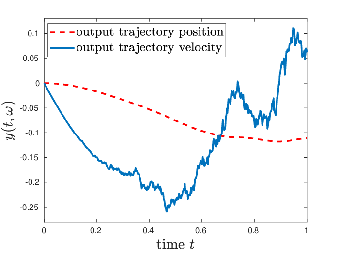
Refer to caption
Figure 1: Trajectory of position and velocity in the middle of the string.
Refer to caption
Figure 2: Trajectory errors between full model and ROM of size r=6r=6.
Refer to caption
Figure 3: Mean errors for position and velocity for r=6r=6.
Refer to caption
Figure 4: Worst case mean error for several dimensions of the ROM.

Figure 2 shows the output trajectory, i.e., the position and the velocity in the middle of the string for one particular sample over the time window [0,1][0,1]. The trajectory of the velocity is as rough as the noise process, whereas the trajectory for the position is smooth as it is the integral of the velocity. Figure 2 plots the respective point-wise errors between the full model of dimension n=1000n=1000 and ROM of dimension r=6r=6 for fixed trajectories. In Figure 4 the expected value of the output error of the full and the reduced model is plotted. Both in Figure 2 for the sample error and in Figure 4 for the mean error we observe that the output error is smaller for the position than for the velocity as this is a smoother function.

Finally, we use Algorithm 1 in order to compute several ROMs of dimensions r=2,…,18r=2,\ldots,18 and the corresponding worst case error supt∈[0,T]𝔼⁡‖y⁡(t)−y^​(t)‖\sup_{t\in[0,T]}\mathbb{E}\left\|y(t)-\hat{y}(t)\right\|, which we plotted in Figure 4. We observe that the error decreases as the size of the ROM increases, as one would expect. We also see that the output error in the position is consistently about one magnitude smaller than the output error in the velocity.

Additive noise

For the additive case in (27) we use α=0.1\alpha=0.1, f1​(z)=cos⁡(2​z)f_{1}(z)=\cos(2z), f2,1​(z)=sin⁡(z)f_{2,1}(z)=\sin(z) and f2,2​(z)=sin⁡(z)​exp⁡(−(z−π/2)2)f_{2,2}(z)=\sin(z)\exp(-(z-\pi/2)^{2}). As input function we take u≡1u\equiv 1, such that ‖u‖LT2=1\|u\|_{L_{T}^{2}}=1. For systems with additive noise (18a) we compare the two approaches considered in this paper for computing a ROM. In this example we only consider the position for the output. Qualitatively we obtain the same results for the velocity, the error is typically larger by one magnitude, as we have seen for the case of multiplicative noise.

Refer to caption
Figure 5: Bounds ℰ1\mathcal{E}_{1}, ℰ2\mathcal{E}_{2} and ℰ3\mathcal{E}_{3} from (21) and (3.2) for different dimensions of the ROM.
Refer to caption
Figure 6: Mean errors for the output when using the one step or two step modified linear IRKA.

First, we use Theorems 2.2 and 2.4 (a) in order to compute the stochastic ℋ2\mathcal{H}_{2}-distance ‖H−H^‖ℒ2​(𝒲)2=tr⁡(C​P​CT)−tr⁡(C^​P^​C^T)\left\|H-\hat{H}\right\|^{2}_{\mathcal{L}^{2}(\mathcal{W})}=\operatorname{tr}(CPC^{T})-\operatorname{tr}(\hat{C}\hat{P}{\hat{C}}^{T}), between a full order model and a ROM for several dimensions of the reduced system, after computing an optimal reduced system of dimensions r=1,…,16r=1,\ldots,16. This allows us to compute ℰ1\mathcal{E}_{1}, ℰ2\mathcal{E}_{2} and ℰ3\mathcal{E}_{3} from (21) and (3.2), which are plotted in Figure 6. Clearly, all errors decrease with increasing size of the ROM. However, we observe that the error ℰ2\mathcal{E}_{2} decreases much more rapidly than the errors ℰ1\mathcal{E}_{1} and ℰ3\mathcal{E}_{3}, which behave similarly. Hence, if we would like to produce a ROM which has an error of at most 2​e−022e-02, we can deduce from Figure 6 that we need r=16r=16 for the first reduced model in (20), r=4r=4 in the second reduced model in (20) and r=16r=16 for the reduced model (23). One can see that there are potential savings by using a smaller reduced dimension and still obtain sufficiently small errors. For this particular case we computed the ROMs both for Algorithm 3 with r=16r=16 and Algorithm 2 with r=16r=16 for the first reduced model and r=4r=4 for the second one. The results are shown in Figure 6. We observe that the worst case mean errors of one step and two step modified linear IRKA are of size 2.99​e−042.99e-04 and 8.20​e−048.20e-04, respectively. The errors are of the same order, despite reducing the subsystem corresponding to the stochastic part to a smaller size.

5 Conclusions

We have derived optimization based model order reduction methods for stochastic systems. In particular we explained the link between the output error for stochastic systems, both with additive and multiplicative noise, and modified versions of the ℋ2\mathcal{H}_{2}-norm for both linear and bilinear deterministic systems. We then developed optimality conditions for minimizing the error bounds computing reduced order models for stochastic systems. This approach revealed that modified versions of iterative rational Krylov methods are in fact natural schemes for reducing large scale stochastic systems with both additive and multiplicative noise. In addition, we have introduced a splitting method for linear systems with additive noise, where the deterministic and the noise part are treated independently. This is advantageous if one of the systems can be reduced easier than the other. It also allows for a different model order reduction method in one of the systems, which we did not discuss in this paper.

Appendix A Ito product rule

In this section, we formulate an Ito product rule for semimartingales on a complete filtered probability space (Ω,ℱ,(ℱt)t≥0,ℙ)\left(\Omega,\mathcal{F},(\mathcal{F}_{t})_{t\geq 0},\mathbb{P}\right). Semimartingales ZZ are stochastic processes that are càdlàg (right-continuous with exiting left limits) that have the representation

Z⁡(t)=M⁡(t)+A⁡(t),t≥0,\displaystyle Z(t)=M(t)+A(t),\quad t\geq 0,

where MM is a càdlàg martingale with respect to (ℱt)t≥0(\mathcal{F}_{t})_{t\geq 0} and AA is a càdlàg process with bounded variation.

Now, let Z1,Z2Z_{1},Z_{2} be scalar semimartingales with jumps Δ​Zi​(s):=Zi​(s)−Zi​(s−)\Delta Z_{i}(s):=Z_{i}(s)-Z_{i}(s-) (i=1,2i=1,2). Then, the Ito product formula is given as follows:

Z1​(t)​Z2​(t)=Z1​(0)​Z2​(0)+∫0tZ1​(s−)​d​Z2​(s)+∫0tZ2​(s−)​d​Z1​(s)+[Z1,Z2]t\displaystyle Z_{1}(t)Z_{2}(t)=Z_{1}(0)Z_{2}(0)+\int_{0}^{t}Z_{1}(s-)dZ_{2}(s)+\int_{0}^{t}Z_{2}(s-)dZ_{1}(s)+[Z_{1},Z_{2}]_{t} (28)

for t≥0t\geq 0, see [21]. By [16, Theorem 4.52], the compensator process [Z1,Z2][Z_{1},Z_{2}] is given by

[Z1,Z2]t=⟨M1c,M2c⟩t+∑0≤s≤tΔ​Z1​(s)​Δ​Z2​(s)\displaystyle[Z_{1},Z_{2}]_{t}=\left\langle M_{1}^{c},M_{2}^{c}\right\rangle_{t}+\sum_{0\leq s\leq t}\Delta Z_{1}(s)\Delta Z_{2}(s) (29)

for t≥0t\geq 0, where M1cM_{1}^{c} and M2cM_{2}^{c} are the square integrable continuous martingale parts of Z1Z_{1} and Z2Z_{2} (cf. [16, Theorem 4.18]). The process ⟨M1c,M2c⟩\left\langle M_{1}^{c},M_{2}^{c}\right\rangle is the uniquely defined angle bracket process that guarantees that M1c​M2c−⟨M1c,M2c⟩M_{1}^{c}M_{2}^{c}-\left\langle M_{1}^{c},M_{2}^{c}\right\rangle is an (ℱt)t≥0(\mathcal{F}_{t})_{t\geq 0}- martingale, see [21, Proposition 17.2]. As a consequence of (28), we obtain the following product rule in the vector valued case.

Lemma A.1.

Let YY be an ℝd\mathbb{R}^{d}-valued and ZZ be an ℝn\mathbb{R}^{n}-valued semimartingale, then we have

Y⁡(t)​ZT​(t)=Y⁡(0)​ZT​(0)+∫0td​Y​(s)​ZT​(s−)+∫0tY⁡(s−)​d​ZT​(s)+([Y(i),Z(j)]t)i=1,…,dj=1,…,n\displaystyle Y(t)Z^{T}(t)=Y(0)Z^{T}(0)+\int_{0}^{t}dY(s)Z^{T}(s-)+\int_{0}^{t}Y(s-)dZ^{T}(s)+\left([Y^{(i)},Z^{(j)}]_{t}\right)_{{i=1,\ldots,d}\atop{j=1,\ldots,n}}

for all t≥0t\geq 0, where Y(i)Y^{(i)} and Z(j)Z^{(j)} are the iith and jjth components of YY and ZZ, respectively.

Appendix B Proof of Lemma 2.1

In order to ease notation, we prove the result for s=0s=0. Let us assume that LL and L^\hat{L} have mm columns denoted by lkl_{k}, l^k\hat{l}_{k}, such that we can decompose L=[l1,…,lm]L=\left[l_{1},\ldots,l_{m}\right] and L^=[l^1,…,l^m]\hat{L}=\left[\hat{l}_{1},\ldots,\hat{l}_{m}\right]. we obtain

Φ⁡(t)​L​L^T​Φ^T​(t)=∑k=1mYk​(t)​ZkT​(t),\displaystyle\Phi(t)L\hat{L}^{T}\hat{\Phi}^{T}(t)=\sum_{k=1}^{m}Y_{k}(t)Z_{k}^{T}(t), (30)

where we set Yk​(t)=Φ⁡(t)​lkY_{k}(t)=\Phi(t)l_{k} and Zk​(t)=Φ^​(t)​l^kZ_{k}(t)=\hat{\Phi}(t)\hat{l}_{k}. We apply Corollary A.1 to every summand of (30). This yields

Yk​(t)​ZkT​(t)=lk​l^kT+∫0td⁡(Yk​(s))​ZkT​(s−)+∫0tYk​(s−)​d​ZkT​(s)+([ei1T​Yk,ei2T​Zk]t)i1=1,…,ni2=1,…,r,\displaystyle Y_{k}(t)Z_{k}^{T}(t)=l_{k}\hat{l}_{k}^{T}+\int_{0}^{t}d(Y_{k}(s))Z_{k}^{T}(s-)+\int_{0}^{t}Y_{k}(s-)dZ_{k}^{T}(s)+\left(\left[e_{i_{1}}^{T}Y_{k},e_{i_{2}}^{T}Z_{k}\right]_{t}\right)_{{i_{1}=1,\ldots,n}\atop{i_{2}=1,\ldots,r}}, (31)

where ei1e_{i_{1}} and ei2e_{i_{2}} are unit vectors of suitable dimension. We determine the expected value of the compensator process of ei1T​Yke_{i_{1}}^{T}Y_{k} and ei2T​Zke_{i_{2}}^{T}Z_{k}. Using (29), it can be seen that this process only depends on the jumps and the continuous martingale parts of YkY_{k} and ZkZ_{k}. Taking (4) and the corresponding equation for the fundamental solution of the reduced system into account, we see that

ℳk​(t):=∑i=1m2∫0tNi​Yk​(s)​d​Mi​(s),ℳ^k​(t):=∑i=1m2∫0tN^i​Zk​(s)​d​Mi​(s)\displaystyle\mathcal{M}_{k}(t):=\sum_{i=1}^{m_{2}}\int_{0}^{t}N_{i}Y_{k}(s)dM_{i}(s),\quad\hat{\mathcal{M}}_{k}(t):=\sum_{i=1}^{m_{2}}\int_{0}^{t}\hat{N}_{i}Z_{k}(s)dM_{i}(s)

are the martingale parts of YkY_{k} and ZkZ_{k} which furthermore contain all the jumps of these processes. This gives

[ei1T​Yk,ei2T​Zk]t=[ei1T​ℳk,ei2T​ℳ^k]t.\displaystyle\left[e_{i_{1}}^{T}Y_{k},e_{i_{2}}^{T}Z_{k}\right]_{t}=\left[e_{i_{1}}^{T}\mathcal{M}_{k},e_{i_{2}}^{T}\hat{\mathcal{M}}_{k}\right]_{t}.

We apply Corollary A.1 to ℳk​ℳ^kT{\mathcal{M}}_{k}\hat{\mathcal{M}}_{k}^{T} and obtain

ℳk​(t)​ℳ^kT​(t)=∫0td⁡(ℳk​(s))​ℳ^kT​(s−)+∫0tℳk​(s−)​d​ℳ^kT​(s)+([ei1T​ℳk,ei2T​ℳ^k]t)i1=1,…,ni2=1,…,r.\displaystyle{\mathcal{M}}_{k}(t)\hat{\mathcal{M}}_{k}^{T}(t)=\int_{0}^{t}d({\mathcal{M}}_{k}(s))\hat{\mathcal{M}}_{k}^{T}(s-)+\int_{0}^{t}{\mathcal{M}}_{k}(s-)d\hat{\mathcal{M}}_{k}^{T}(s)+\left(\left[e_{i_{1}}^{T}{\mathcal{M}}_{k},e_{i_{2}}^{T}\hat{\mathcal{M}}_{k}\right]_{t}\right)_{{i_{1}=1,\ldots,n}\atop{i_{2}=1,\ldots,r}}.

Since ℳk{\mathcal{M}}_{k} and ℳ^k\hat{\mathcal{M}}_{k} are mean zero martingales [23], the above integrals with respect to these processes have mean zero as well [18]. Hence, we have

𝔼⁡[ℳk​(t)​ℳ^kT​(t)]=𝔼​([ei1T​ℳk,ei2T​ℳ^k]t)i1=1,…,ni2=1,…,r=𝔼​([ei1T​Yk,ei2T​Zk]t)i1=1,…,ni2=1,…,r.\displaystyle\mathbb{E}[{\mathcal{M}}_{k}(t)\hat{\mathcal{M}}_{k}^{T}(t)]=\mathbb{E}\left(\left[e_{i_{1}}^{T}{\mathcal{M}}_{k},e_{i_{2}}^{T}\hat{\mathcal{M}}_{k}\right]_{t}\right)_{{i_{1}=1,\ldots,n}\atop{i_{2}=1,\ldots,r}}=\mathbb{E}\left(\left[e_{i_{1}}^{T}Y_{k},e_{i_{2}}^{T}Z_{k}\right]_{t}\right)_{{i_{1}=1,\ldots,n}\atop{i_{2}=1,\ldots,r}}.

We apply the expected value to both sides of (31) leading to

𝔼⁡[Yk​(t)​ZkT​(t)]=lk​l^kT+𝔼⁡[∫0td⁡(Yk​(s))​ZkT​(s−)]+𝔼⁡[∫0tYk​(s−)​d​ZkT​(s)]+𝔼⁡[ℳk​(t)​ℳ^kT​(t)].\displaystyle\mathbb{E}[Y_{k}(t)Z_{k}^{T}(t)]=l_{k}\hat{l}_{k}^{T}+\mathbb{E}\left[\int_{0}^{t}d(Y_{k}(s))Z_{k}^{T}(s-)\right]+\mathbb{E}\left[\int_{0}^{t}Y_{k}(s-)dZ_{k}^{T}(s)\right]+\mathbb{E}[{\mathcal{M}}_{k}(t)\hat{\mathcal{M}}_{k}^{T}(t)].

We insert d​YkdY_{k} and d​ZkdZ_{k} (given through (4)) into the above equation and exploit that an Ito integral has mean zero, and obtain

𝔼⁡[Yk​(t)​ZkT​(t)]=lk​l^kT+∫0tA​𝔼​[Yk​(s)​ZkT​(s)]​𝑑s+∫0t𝔼⁡[Yk​(s)​ZkT​(s)]​A^T​𝑑s+𝔼⁡[ℳk​(t)​ℳ^kT​(t)].\displaystyle\mathbb{E}[Y_{k}(t)Z_{k}^{T}(t)]=l_{k}\hat{l}_{k}^{T}+\int_{0}^{t}A\mathbb{E}\left[Y_{k}(s)Z_{k}^{T}(s)\right]ds+\int_{0}^{t}\mathbb{E}\left[Y_{k}(s)Z_{k}^{T}(s)\right]\hat{A}^{T}ds+\mathbb{E}[{\mathcal{M}}_{k}(t)\hat{\mathcal{M}}_{k}^{T}(t)].

Notice that we replaced the left limits by the function values above and hence changed the integrand only on Lebesgue zero sets since the processes have only countably many jumps on bounded time intervals [3]. The Ito isometry [23] now yields

𝔼⁡[ℳk​(t)​ℳ^kT​(t)]=∑i,j=1m2∫0tNi​𝔼​[Yk​(s)​ZkT​(s)]​N^jT​ki​j​𝑑s.\displaystyle\mathbb{E}[{\mathcal{M}}_{k}(t)\hat{\mathcal{M}}_{k}^{T}(t)]=\sum_{i,j=1}^{m_{2}}\int_{0}^{t}N_{i}\mathbb{E}[Y_{k}(s)Z_{k}^{T}(s)]\hat{N}_{j}^{T}k_{ij}ds.

Combining this result with (30) proves the claim of this lemma.

Appendix C Proof of Theorem 2.5

We only show the result for the optimality condition (c) in (13). All the other optimality conditions (a), (b) and (d) are derived similarly. We first reformulate optimality condition (c). Defining Ψ^i:=∑j=1m2N^j​ki​j\hat{\Psi}_{i}:=\sum_{j=1}^{m_{2}}{\hat{N}}_{j}k_{ij} and Ψi:=∑j=1m2Nj​ki​j\Psi_{i}:=\sum_{j=1}^{m_{2}}{N}_{j}k_{ij} for i=1,…,m2i=1,\ldots,m_{2}, we have that

Q^​Ψ^i​P^=Q2​Ψi​P2⇔(S−T​Q^)​Ψ^i​(P^​ST)=(S−T​Q2)​Ψi​(P2​ST)\displaystyle\hat{Q}\hat{\Psi}_{i}\hat{P}=Q_{2}\Psi_{i}P_{2}\Leftrightarrow(S^{-T}\hat{Q})\hat{\Psi}_{i}(\hat{P}S^{T})=(S^{-T}Q_{2})\Psi_{i}(P_{2}S^{T})
⇔tr((S−TQ^)Ψ^i(P^ST)emekT)=tr((S−TQ2)Ψi(P2ST)emekT)∀k,m=1,…,r,\displaystyle\Leftrightarrow\operatorname{tr}\left((S^{-T}\hat{Q})\hat{\Psi}_{i}(\hat{P}S^{T})e_{m}e_{k}^{T}\right)=\operatorname{tr}\left((S^{-T}Q_{2})\Psi_{i}(P_{2}S^{T})e_{m}e_{k}^{T}\right)\quad\forall k,m=1,\ldots,r,

where SS is the factor of the spectral decomposition of A^\hat{A}. Using the relation between the trace and the vectorization vec⁡(⋅)\operatorname{vec}(\cdot) of a matrix as well as the Kronecker product ⊗\otimes of two matrices, we obtain an equivalent formulation of the optimality condition (c) in (13), i.e. Q^​Ψ^i​P^=Q2​Ψi​P2\hat{Q}\hat{\Psi}_{i}\hat{P}=Q_{2}\Psi_{i}P_{2} is equivalent to

⇔vecT⁡(Q^​S−1)​(ek​emT⊗Ψ^i)​vec⁡(P^​ST)=vecT⁡(Q2T​S−1)​(ek​emT⊗Ψi)​vec⁡(P2​ST)\displaystyle\Leftrightarrow\operatorname{vec}^{T}(\hat{Q}S^{-1})(e_{k}e_{m}^{T}\otimes\hat{\Psi}_{i})\operatorname{vec}(\hat{P}S^{T})=\operatorname{vec}^{T}(Q_{2}^{T}S^{-1})(e_{k}e_{m}^{T}\otimes\Psi_{i})\operatorname{vec}(P_{2}S^{T}) (32)

for all k,m=1,…,rk,m=1,\ldots,r. We now use Algorithm 1 to show that this equality holds. We multiply (10) with STS^{T} and (14) with S−1S^{-1} from the right to find the equations for P^​ST\hat{P}S^{T} and Q^​S−1\hat{Q}S^{-1}. Subsequently, we vectorize these equations and get

vec⁡(Q^​S−1)\displaystyle\operatorname{vec}(\hat{Q}S^{-1}) =−𝒦^−Tvec(C^TC~)and\displaystyle=-\hat{\mathcal{K}}^{-T}\operatorname{vec}(\hat{C}^{T}\tilde{C})\quad\text{and} (33)
vec⁡(P^​ST)\displaystyle\operatorname{vec}(\hat{P}S^{T}) =−𝒦^−1​vec⁡(B^1​𝒲​(B~1​𝒲)T),\displaystyle=-\hat{\mathcal{K}}^{-1}\operatorname{vec}(\hat{B}_{1}\mathcal{W}(\tilde{B}_{1}\mathcal{W})^{T}), (34)

where 𝒦^:=(I⊗A^)+(D⊗I)+∑i,j=1m2(N~i⊗N^j)​ki​j\hat{\mathcal{K}}:=(I\otimes\hat{A})+(D\otimes I)+\sum_{i,j=1}^{m_{2}}(\tilde{N}_{i}\otimes\hat{N}_{j})k_{ij} and recalling that D=S​A^​S−1,B~1=S​B^1,C~=C^​S−1,N~i=S​N^i​S−1D=S\hat{A}S^{-1},~\tilde{B}_{1}=S\hat{B}_{1},~\tilde{C}=\hat{C}S^{-1},~\tilde{N}_{i}=S\hat{N}_{i}S^{-1}.

With 𝒦:=(I⊗A)+(D⊗I)+∑i,j=1m2(N~i⊗Nj)​ki​j{\mathcal{K}}:=(I\otimes A)+(D\otimes I)+\sum_{i,j=1}^{m_{2}}(\tilde{N}_{i}\otimes N_{j})k_{ij}, and the definition of the reduced matrices A^=(WT​V)−1​WT​A​V\hat{A}=(W^{T}V)^{-1}W^{T}AV, B^1=(WT​V)−1​WT​B1\hat{B}_{1}=(W^{T}V)^{-1}W^{T}B_{1}, C^=C​V\hat{C}=CV and N^i=(WT​V)−1​WT​Ni​V\hat{N}_{i}=(W^{T}V)^{-1}W^{T}N_{i}V in Algorithm 1 we furthermore have that

−vec⁡(C^T​C~)\displaystyle-\operatorname{vec}(\hat{C}^{T}\tilde{C}) =−vec⁡(VT​CT​C~)=−(I⊗VT)​vec⁡(CT​C~)=(I⊗VT)​𝒦T​vec⁡(W)\displaystyle=-\operatorname{vec}(V^{T}C^{T}\tilde{C})=-(I\otimes V^{T})\operatorname{vec}(C^{T}\tilde{C})=(I\otimes V^{T})\mathcal{K}^{T}\operatorname{vec}(W)
=(I⊗VT)​𝒦T​vec⁡(W​(VT​W)−1​VT​W)\displaystyle=(I\otimes V^{T})\mathcal{K}^{T}\operatorname{vec}(W(V^{T}W)^{-1}V^{T}W)
=(I⊗VT)​𝒦T​(I⊗W​(VT​W)−1​VT)​vec⁡(W)=𝒦^T​(I⊗VT)​vec⁡(W)\displaystyle=(I\otimes V^{T})\mathcal{K}^{T}(I\otimes W(V^{T}W)^{-1}V^{T})\operatorname{vec}(W)=\hat{\mathcal{K}}^{T}(I\otimes V^{T})\operatorname{vec}(W)

and

−vec⁡(B^1​𝒲​(B~1​𝒲)T)\displaystyle-\operatorname{vec}(\hat{B}_{1}\mathcal{W}(\tilde{B}_{1}\mathcal{W})^{T}) =−vec⁡((WT​V)−1​WT​B1​𝒲​(B~1​𝒲)T)\displaystyle=-\operatorname{vec}((W^{T}V)^{-1}W^{T}B_{1}\mathcal{W}(\tilde{B}_{1}\mathcal{W})^{T})
=−(I⊗(WT​V)−1​WT)​vec⁡(B1​𝒲​(B~1​𝒲)T)\displaystyle=-(I\otimes(W^{T}V)^{-1}W^{T})\operatorname{vec}(B_{1}\mathcal{W}(\tilde{B}_{1}\mathcal{W})^{T})
=(I⊗(WT​V)−1​WT)​𝒦​vec⁡(V)\displaystyle=(I\otimes(W^{T}V)^{-1}W^{T})\mathcal{K}\operatorname{vec}(V)
=(I⊗(WT​V)−1​WT)​𝒦​vec⁡(V​(WT​V)−1​WT​V)\displaystyle=(I\otimes(W^{T}V)^{-1}W^{T})\mathcal{K}\operatorname{vec}(V(W^{T}V)^{-1}W^{T}V)
=(I⊗(WT​V)−1​WT)​𝒦​(I⊗V​(WT​V)−1​WT)​vec⁡(V)\displaystyle=(I\otimes(W^{T}V)^{-1}W^{T})\mathcal{K}(I\otimes V(W^{T}V)^{-1}W^{T})\operatorname{vec}(V)
=𝒦^​(I⊗(WT​V)−1​WT)​vec⁡(V)\displaystyle=\hat{\mathcal{K}}(I\otimes(W^{T}V)^{-1}W^{T})\operatorname{vec}(V)

We insert both results into (33) and obtain expressions for vec⁡(Q^​S−1)\operatorname{vec}(\hat{Q}S^{-1}) and vec⁡(P^​ST)\operatorname{vec}(\hat{P}S^{T}) in terms of the projection matrices from Algorithm 1:

vec⁡(Q^​S−1)=(I⊗VT)​vec⁡(W)andvec⁡(P^​ST)=(I⊗(WT​V)−1​WT)​vec⁡(V).\displaystyle\operatorname{vec}(\hat{Q}S^{-1})=(I\otimes V^{T})\operatorname{vec}(W)\quad\text{and}\quad\operatorname{vec}(\hat{P}S^{T})=(I\otimes(W^{T}V)^{-1}W^{T})\operatorname{vec}(V).

Hence, the left hand side of the optimality condition (32) can be written as

vecT⁡(Q^​S−1)​(ek​emT⊗Ψ^i)​vec⁡(P^​ST)\displaystyle\operatorname{vec}^{T}(\hat{Q}S^{-1})(e_{k}e_{m}^{T}\otimes\hat{\Psi}_{i})\operatorname{vec}(\hat{P}S^{T})
=vecT⁡(W)​(I⊗V)​(ek​emT⊗Ψ^i)​(I⊗(WT​V)−1​WT)​vec⁡(V)\displaystyle=\operatorname{vec}^{T}(W)(I\otimes V)(e_{k}e_{m}^{T}\otimes\hat{\Psi}_{i})(I\otimes(W^{T}V)^{-1}W^{T})\operatorname{vec}(V)
OPEN=vecT⁡(W)​(I⊗V​(WT​V)−1​WT))​(ek​emT⊗Ψi)​(I⊗V​(WT​V)−1​WT)​vec⁡(V)\displaystyle=\operatorname{vec}^{T}(W)(I\otimes V(W^{T}V)^{-1}W^{T}))(e_{k}e_{m}^{T}\otimes\Psi_{i})(I\otimes V(W^{T}V)^{-1}W^{T})\operatorname{vec}(V)
=vecT⁡(W)​(ek​emT⊗Ψi)​vec⁡(V),\displaystyle=\operatorname{vec}^{T}(W)(e_{k}e_{m}^{T}\otimes\Psi_{i})\operatorname{vec}(V),

where we have used properties of the Kronecker product again. It remains to show that P2​ST=VP_{2}S^{T}=V and Q2T​S−1=WQ_{2}^{T}S^{-1}=W for the optimality condition to hold. This is obtained by multiplying (11) with STS^{T} from the right and (15) with S−TS^{-T} from the left. Hence (32) holds which concludes the proof.

References

  • [1] B. Anić, C. Beattie, S. Gugercin, and A.C. Antoulas. Interpolatory weighted-ℋ2\mathcal{H}_{2} model reduction. Automatica, 49(5):1275–1280, 2013.
  • [2] A.C. Antoulas. Approximation of large-scale dynamical systems. Advances in Design and Control 6. Philadelphia, PA: SIAM, 2005.
  • [3] D. Applebaum. Lévy Processes and Stochastic Calculus. 2nd ed. Cambridge Studies in Advanced Mathematics 116. Cambridge: Cambridge University Press, 2009.
  • [4] S. Becker and C. Hartmann. Infinite-dimensional bilinear and stochastic balanced truncation with explicit error bounds. Mathematics of Control, Signals, and Systems, 31(2):1–37, 2019.
  • [5] S. Becker, C. Hartmann, M. Redmann, and L. Richter. Feedback control theory & Model order reduction for stochastic equations. arXiv preprint 1912.06113, 2019.
  • [6] P. Benner and T. Breiten. Interpolation-based ℋ2\mathcal{H}_{2}-model reduction of bilinear control systems. SIAM J. Matrix Anal. Appl, 33(3):859–885, 2012.
  • [7] P. Benner and T. Damm. Lyapunov equations, energy functionals, and model order reduction of bilinear and stochastic systems. SIAM J. Control Optim., 49(2):686–711, 2011.
  • [8] P. Benner and M. Redmann. Model Reduction for Stochastic Systems. Stoch PDE: Anal Comp, 3(3):291–338, 2015.
  • [9] T. Breiten, C. Beattie, and S. Gugercin. Near-optimal frequency-weighted interpolatory model reduction. System & Control Letters, 78:8–18, 2015.
  • [10] T. Damm and P. Benner. Balanced truncation for stochastic linear systems with guaranteed error bound. Proceedings of MTNS–2014, Groningen, The Netherlands, pages 1492–1497, 2014.
  • [11] G. Flagg and S. Gugercin. Multipoint volterra series interpolation and ℋ2\mathcal{H}_{2} optimal model reduction of bilinear systems. SIAM J. Matrix Anal. Appl, 36(2):549–579, 2015.
  • [12] S. Gugercin, A.C. Antoulas, and C. Beattie. ℋ2\mathcal{H}_{2} Model Reduction for Large-Scale Linear Dynamical System. SIAM J. Matrix Anal. Appl, 30(2):609–638, 2008.
  • [13] Y. Halevi. Frequency weighted model reduction via optimal projection. IEEE Trans. Automat. Control, 37(10):1537–1542, 1992.
  • [14] C. Hartmann. Balanced model reduction of partially observed langevin equations: an averaging principle. Math. Comput. Model. Dyn. Syst., 17(5):463–490, 2011.
  • [15] D. Hyland and D. Bernstein. The optimal projection equations for model reduction and the relationships among the methods of Wilson, Skelton, and Moore. IEEE Transactions on Automatic Control,, 30(12):1201–1211, 1985.
  • [16] J. Jacod and A.N. Shiryaev. Limit Theorems for Stochastic Processes. 2nd ed. Grundlehren der Mathematischen Wissenschaften. 288. Berlin: Springer, 2003.
  • [17] R.Z. Khasminskii. Stochastic stability of differential equations. Monographs and Textbooks on Mechanics of Solids and Fluids. Mechanics: Analysis, 7. Alphen aan den Rijn, The Netherlands; Rockville, Maryland, USA: Sijthoff & Noordhoff., 1980.
  • [18] H.-H. Kuo. Introduction to Stochastic Integration. Universitext. New York, NJ: Springer, 2006.
  • [19] L. Meier and D. Luenberger. Approximation of linear constant systems. IEEE Transactions on Automatic Control, 12(5):585—588, 1967.
  • [20] Y. Liu and B.D.O. Anderson. Singular perturbation approximation of balanced systems. Int. J. Control, 50(4):1379–1405, 1989.
  • [21] M. Metivier. Semimartingales: A Course on Stochastic Processes. De Gruyter Studies in Mathematics, 2. Berlin - New York: de Gruyter, 1982.
  • [22] B.C. Moore. Principal component analysis in linear systems: Controllability, observability, and model reduction. IEEE Trans. Autom. Control, 26:17–32, 1981.
  • [23] S. Peszat and J. Zabczyk. Stochastic Partial Differential Equations with Lévy Noise. An evolution equation approach. Encyclopedia of Mathematics and Its Applications 113. Cambridge: Cambridge University Press, 2007.
  • [24] M. Redmann. Type II singular perturbation approximation for linear systems with Lévy noise. SIAM J. Control Optim., 56(3):2120–2158., 2018.
  • [25] M. Redmann. The missing link between the output and the ℋ2\mathcal{H}_{2}-norm of bilinear systems. arXiv e-print:1910.14427, 2019.
  • [26] M. Redmann and P. Benner. Approximation and Model Order Reduction for Second Order Systems with Lévy-Noise. AIMS Proceedings, pages 945–953, 2015.
  • [27] M. Redmann and P. Benner. Singular Perturbation Approximation for Linear Systems with Lévy Noise. Stochastics and Dynamics, 18(4), 2018.
  • [28] M. Redmann and M.A. Freitag. Balanced model order reduction for linear random dynamical systems driven by Lévy-Noise. J. Comput. Dyn., 5(1&2):33–59, 2018.
  • [29] D.A. Wilson. Optimum solution of model-reduction problem. In Proceedings of the Institution of Electrical Engineers, volume 117, pages 1161–1165. IET, 1970.
  • [30] L. Zhang and J. Lam. On H2H_{2} model reduction of bilinear systems. Automatica, 38(2):205–216, 2002.