Nested Hybrid Cylindrical Array Design and DoA Estimation for Massive IoT NetworksThanks: This work was supported in part by the National Natural Science Foundation of China (NSFC) under Grants 61671072, and in part by the Beijing Natural Science Foundation under Grants L192025. (Corresponding author: Tiejun Lv.) Z. Lin and T. Lv are with the School of Information and Communication Engineering, BUPT, Beijing, China (email: {linlzp, lvtiejun}@bupt.edu.cn). Z. Lin is also with the School of Electrical and Data Engineering, UTS, Sydney, Australia. W. Ni is with the Data61, CSIRO, Sydney, Australia (e-mail: Wei.Ni@data61.csiro.au). J. A. Zhang and R. P. Liu are with the School of Electrical and Data Engineering, UTS, Sydney, Australia (e-mail: {Andrew.Zhang, RenPing.Liu}@uts.edu.au).

According to (10), the element positions of the difference coarray are the (self) differences between the locations of original physical antenna elements.

Based on the definition of difference coarray, we can define a cross difference coarray, which corresponds to the cross differences between the element locations of two arrays with $N$ and $M$ elements:

According to (10) and (11), we can see that the concept of difference coarray arises naturally in the second-order statistics of the impinging signals. For example, we consider that a signal $\mathbf{x}_{\mathbf{w}_{n}}\in\mathbb{C}^{N\times 1}$ is received at the $n$-th element of an antenna array. The cross-correlation between the signals received at the $n_{1}$-th and $n_{2}$-th elements of the array is given by

where $\mathbf{R}_{(\mathbf{w}_{n_{1}}-\mathbf{w}_{n_{2}})}$ can be viewed as a signal sample received by a (larger) difference coarray with virtual array elements located at $(\mathbf{w}_{n_{1}}-\mathbf{w}_{n_{2}})\in\mathbb{D}_{\textrm{dc}}$ [12].

By adequately designing the element locations, i.e., $\mathbb{D}_{\textrm{a}}$, we can increase the number of virtual elements in the difference coarray after computing the autocorrelation. If we use the samples from the difference coarray to perform spectral estimation, the parameters of much more targets can be estimated.

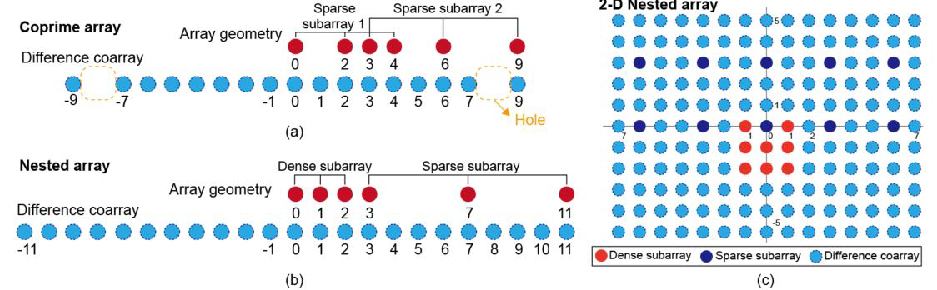
We proceed to introduce the concept of sparse array. An array is said to be sparse if the spacing between a majority or all of adjacent elements is more than one (half-wavelength) [12, 15]. By applying the concept of sparse array to antenna design, we can significantly improve the number of distinguishable targets using a small number of physical antenna elements [27]. Some well-known 1-D sparse arrays include MRA [13], MHA [14], nested arrays [12], and coprime arrays [15]. With $O(N)$ physical array elements, both MRA and MHA can construct difference coarrays with the size of $O(N^{2})$. However, their geometries need to be constructed by using searching algorithms, e.g., integer programming [14, 28]. Nested and coprime arrays were proposed in [12, 15] with closed-form expressions for element locations, and both of them can construct difference coarrays with the same DoF as MRA and MHA. An example of nested and coprime arrays, and their difference coarrays are shown in Figs. 2(a) and 2(b). Nested arrays can offer larger difference coarray DoF than coprime arrays, as shown in Fig. 2(b), where both of them have six physical elements. In addition, the difference coarrays of nested arrays consist of evenly spaced virtual elements with no holes, so that the subspace-based estimation algorithms, such as MUSIC and ESPRIT, can be utilized on the coarray domain without creating ambiguities [28]. For the details of these arrays, interested readers can refer to [13, 14, 12, 15].

In the next subsection, we design the phase shifter matrix $\mathbf{B}_{\textrm{ps}}$. $\mathbf{B}_{\textrm{ps}}$ can transform the UCyA steering vectors from the element space into a phase space, where the phases of the array steering vectors are linear to the element locations. From (12), we see that if we want to construct a difference coarray with a similar geometry to that of the original array, e.g., the UCyA in our system, the phase of the array steering vectors should vary linearly with the element locations. However, due to the special geometry of the UCyA, if we directly calculate the cross correlation of the array steering vectors, it would generate a virtual non-UCyA composed of multiple non-UCAs [24], leading to an increased computational complexity and degraded the estimation accuracy.

The analog beamforming matrix $\mathbf{B}_{\textrm{rf}}=\mathbf{B}_{\textrm{ps}}\mathbf{B}_{\textrm{rfc}}\in\mathbb{C}^{M_{\textrm{bs}}\times M_{\textrm{rf}}}$ is composed of a phase shifter matrix $\mathbf{B}_{\textrm{ps}}\in\mathbb{C}^{M_{\textrm{bs}}\times M_{\textrm{bsr}}}$ and an RF-chain connection matrix $\mathbf{B}_{\textrm{rfc}}\in\mathbb{C}^{M_{\textrm{bsr}}\times M_{\textrm{rf}}}$, where $M_{\textrm{bsr}}$ is the number of output ports of the phase-shifter matrix. An illustration of the RF front-end structure is shown in Fig. 3. Here, we design $\mathbf{B}_{\textrm{ps}}$ based on circular phase-space transformation [29], to transform the nonlinear phase of UCyA steering vectors to be linear to the element locations.

We decouple $\mathbf{B}_{\textrm{{ps}}}$ between the vertical and horizontal planes, i.e., $\mathbf{B}_{\textrm{ps}}=\mathbf{B}_{\textrm{vps}}\otimes\mathbf{B}_{\textrm{hps}}$ with $\mathbf{B}_{\textrm{vps}}\in\mathbb{C}^{M_{\textrm{v}}\times M_{\textrm{vr}}}$ and $\mathbf{B}_{\textrm{hps}}\in\mathbb{C}^{M_{\textrm{h}}\times M_{\textrm{hr}}}$, and thus $M_{\textrm{bsr}}=M_{\textrm{vr}}M_{\textrm{hr}}$, where $M_{\textrm{vr}}$ and $M_{\textrm{hr}}$ are the number of the phase-shifter output ports along the vertical and horizontal directions, respectively. According to the phase-space transformation of UCAs [29], we design $\mathbf{B}_{\textrm{hps}}$ as $\left[\mathbf{B}_{\textrm{hps}}\right]_{m_{\textrm{h}},m_{\textrm{hr}}+P+1}=e^{-j\frac{2\pi(m_{\textrm{h}}-1)}{M_{\textrm{h}}}m_{\textrm{hr}}},$ where $M_{\textrm{hr}}=2P+1$, $m_{\textrm{hr}}=-P,-P+1,\ldots,P$, and $P$ is the highest phase-space dimension. Thus, the $M_{\textrm{h}}$-dimensional array steering vector $\mathbf{a}_{\textrm{h}}(\theta_{k},\phi_{k})$ can be transformed into a $(2P+1)$-dimensional phase space, i.e., $\mathbf{a}_{\textrm{hps}}(\theta_{k},\phi_{k})=\mathbf{B}_{\textrm{hps}}^{H}\mathbf{a}_{\textrm{h}}(\theta_{k},\phi_{k})\in\mathbb{C}^{(2P+1)\times 1}$. The value of the highest phase-space dimension, $P$, can be configured based on the following theorem.

We set $\mathbf{B}_{\textrm{vps}}=\mathbf{I}_{M_{\textrm{v}}}$ to preserve the recurrence relations among UCAs. According to Theorem 1, the array steering vectors $\mathbf{a}_{\textrm{bs}}(\theta_{k},\phi_{k})$ after the hybrid beamformer is given by

where $\mathbf{B}_{\textrm{bb}}$ is a diagonal matrix used to guarantee the power constraint [30]. Without loss of generality, we set $\mathbf{B}_{\textrm{bb}}=\mathbf{I}_{M_{\textrm{bsr}}}$ in this paper. According to two properties of the Khatri-Rao product: $(\mathbf{A}\otimes\mathbf{B})^{H}=\mathbf{A}^{H}\otimes\mathbf{B}^{H}$ and $(\mathbf{A}\otimes\mathbf{B})(\mathbf{C}\otimes\mathbf{D})=\mathbf{AC}\otimes\mathbf{BD}$ [31], (14) can be rewritten as

where $\mathbf{a}_{\textrm{vps}}(\theta_{k})\in\mathbb{C}^{M_{\textrm{vr}}\times 1}$, $\mathbf{a}_{\textrm{hps}}(\theta_{k},\phi_{k})\in\mathbb{C}^{M_{\textrm{hr}}\times 1}$, $M_{\textrm{vr}}=M_{\textrm{v}}$, and $M_{\textrm{hr}}=2P+1$.

According to Theorem 1, we have

From (16) and (17), we see that, through the proposed $\mathbf{B}_{\textrm{ps}}$, the phases of the array steering vectors become linear to the element locations. This is important to exploit the property of the sparse array theory to design the RF-chain connection matrix $\mathbf{B}_{\textrm{rfc}}$.

In this subsection, we apply the sparse array technique to design $\mathbf{B}_{\textrm{rfc}}$, which enables the DoAs of a large number of devices to be estimated with a marginal accuracy loss while significantly reducing the number of required RF chains. We aim to use as few RF chains as possible to achieve the same, or even larger, DoF than the fully connected beamforming array³³ 3 Due to the use of phase shifter network, the antenna DoF of UCyA depends on the scale of the phase shifter network. Thus, if we use a fully connected beamforming array, $(2P+1)M_{\textrm{v}}$ RF chains are needed, which can provide $\mathcal{O}(PM_{\textrm{v}})$ DoFs. . This objective is different from the previous sparse array researches, which have typically focused on maximizing the size of difference coarrays under the constraint of a fixed number of physical antenna elements.

We first flatten the 3-D RF-chain connection network of UCyA into a 2-D plane, as shown in Fig. 4, by disjoining the RF-chain connection network at the first column phase shifters of every UCA. Different from typical 2-D arrays, due to the periodicity of UCAs, the first and the last phase-shifter output ports of every row in the flattened 2-D RF-chain connection network are identical, as shown in Fig. 4, where the dotted circles denote the last-column phase shifters.

After the flattening processing, the 3-D RF-chain connection network becomes a quasi-2D rectangular array with size of $(M_{\textrm{hr}}+1)\times M_{\textrm{vr}}$, where the increased dimension is due to the repeated phase-shifter output ports, as shown in Fig. 4. The idea of 2-D sparse arrays can be applied to design a 3-D RF-chain connection network of UCyA⁴⁴ 4 Although the RF-chain connection network actually does not have the exact shape, according to the array steering vectors in (16) and (17), we can also regard the network as an UCyA.. In this paper, we design the RF-chain connection network based on a 2-D nested array. This is because (1) a nested array can generate larger hole-free difference coarrays than a coprime array under the same setting, as discussed in Section III-A; and (2) it has simple closed-form expressions for a large number of elements, which cannot be achieved in MRA and MHA. There are also some other frequently-used 2-D sparse arrays, e.g., hourglass arrays and open box arrays (OBAs) [28, 32]. We will compare the RF-chain connection networks designed based on those array geometries with our design in Section V-C.

Our proposed sparse RF-chain connection network is developed from the “Configuration II” nested array [17]. In the general “Configuration II” nested array, when there are $N_{\textrm{dense}}=N_{\textrm{vd}}N_{\textrm{hd}}-1$ and $N_{\textrm{sparse}}=N_{\textrm{vs}}N_{\textrm{hs}}$ elements in the dense and sparse subarrays, respectively, the constructed hole-free difference coarray has $N_{\textrm{dc}}=N_{\textrm{vdc}}N_{\textrm{hdc}}=(2N_{\textrm{vd}}N_{\textrm{vs}}-1)N_{\textrm{hd}}N_{\textrm{hs}}$ elements [17], as shown in Fig. 2(c). Here, $N_{\textrm{vd}}$ and $N_{\textrm{hd}}$ are the numbers of elements in the dense subarray along the vertical and horizontal directions, respectively; $N_{\textrm{vs}}$ and $N_{\textrm{hs}}$ are the numbers of elements in the sparse subarray along the vertical and horizontal directions, respectively; and $N_{\textrm{vdc}}$ and $N_{\textrm{hdc}}$ are the numbers of elements in the difference coarray along the vertical and horizontal directions, respectively. We wish to find the distribution of the RF chains between the sparse and the dense arrays that use as few RF chains as possible to achieve the same DoF as the fully connected beamforming array.

Due to the above-mentioned periodicity of UCAs, when we apply the sparse array technique into our hybrid front-end design, two cases need to be considered for UCyAs. Fig. 5(a) shows the first case, where the first and the last columns of the difference coarray overlap. From Fig. 5(a), we can see that because one column (first or last) of the difference coarray is redundant, two elements of the sparse subarray can be omitted to reduce the element number. A drawback is that this case requires $M_{\textrm{hr}}=(N_{\textrm{hs}}-1)N_{\textrm{hd}}$, which would impose a strict requirement on the number of phase shifters on the horizontal plane. The second case is shown in Fig. 5(b), which requires the constructed difference coarray to be larger than the original UCyA, to achieve the same DoF as a fully connected beamforming array on the horizontal space. In this case, $N_{\textrm{hd}}N_{\textrm{hs}}\geq M_{\textrm{hr}}>(N_{\textrm{hs}}-1)N_{\textrm{hd}}/2$.

In our system, due to the new phase shifter network designed in Section III-B, we have $M_{\textrm{hr}}=2P+1$ (which is an odd number). Since in the Configuration II nested array, the dense and sparse subarrays are symmetric, i.e., both $N_{\textrm{hs}}$ and $N_{\textrm{hd}}$ are odd, we have $(N_{\textrm{hs}}-1)N_{\textrm{hd}}$ is even, and only the above-mentioned second case needs to be considered in our system. We formulate the optimization problem as

(C1) and (C2) guarantee the DoF requirements for the constructed difference coarray of the RF-chain connection network. (C3) avoids solutions that degenerate to 1-D arrays. (C4) is due to the fact that the dense array in Configuration II is symmetrical, and $N_{\textrm{hd}}$ and $N_{\textrm{vd}}$ are invariant factors [18] of the array distribution matrix.

The solution for (18) can be obtained by adopting the following strategy. According to (C1) and (C2), since $N_{\textrm{vs}},N_{\textrm{hs}}\in\mathbb{Z}^{+}$, we can obtain $N_{\textrm{vs}}=\left\lceil(M_{\textrm{vr}}-1)/2N_{\textrm{vd}}\right\rceil$ and $N_{\textrm{hs}}=\left\lceil M_{\textrm{hr}}/N_{\textrm{hd}}\right\rceil$. The optimization problem (18) becomes

Given $M_{\textrm{vr}}$ and $M_{\textrm{hr}}$, we see that (19) exhibits the form of $y=x+\frac{a}{x}$, where $a>0$ is a constant and $y=x+\frac{a}{x}\geq 2\sqrt{a}$. Because $y=2\sqrt{a}$ iff $x=\frac{a}{x}$, the minimum $M_{\textrm{rf}}$ can be obtained when the difference between $N_{\textrm{vd}}N_{\textrm{hd}}$ and $\left\lceil(M_{\textrm{vr}}-1)/2N_{\textrm{vd}}\right\rceil\left\lceil M_{\textrm{hr}}/N_{\textrm{hd}}\right\rceil$ is the smallest. Since $N_{\textrm{vd}},N_{\textrm{hd}},N_{\textrm{vs}},N_{\textrm{hs}}\in\mathbb{Z}^{+}$, we can determine the approximate value ranges of $N_{\textrm{vd}}N_{\textrm{hd}}$ and $\left\lceil(M_{\textrm{vr}}-1)/2N_{\textrm{vd}}\right\rceil\left\lceil M_{\textrm{hr}}/N_{\textrm{hd}}\right\rceil$, and (19) is an integer programming problem. According to (C3) and (C4), the optimal solutions of $N_{\textrm{vd}},N_{\textrm{hd}},N_{\textrm{vs}},$ and $N_{\textrm{hs}}$ to (19) can be obtained by using brute-force search with the value range between $N_{\textrm{vd}}N_{\textrm{hd}}$ and $\left\lceil(M_{\textrm{vr}}-1)/2N_{\textrm{vd}}\right\rceil\left\lceil M_{\textrm{hr}}/N_{\textrm{hd}}\right\rceil$.

In the proposed sparse RF-chain connection network, the RF chains only need to connect the phase shifters located in the dense and sparse subarrays. Based on the calculated values of $N_{\textrm{vd}},N_{\textrm{hd}},N_{\textrm{vs}},$ and $N_{\textrm{hs}}$, now we provide the element locations in the dense and sparse arrays. For illustration convenience, we define the overlapping point of the sparse and dense arrays as the origin of the nested array⁵⁵ 5 Because the parameter estimation depends on the difference between array elements, the changed absolute positions of array elements does not effect the estimation performance.. Let $\mathbf{m}_{\textrm{sp}}=(m_{\textrm{v\_sp}},m_{\textrm{h\_sp}})$ and $\mathbf{m}_{\textrm{de}}=(m_{\textrm{v\_de}},m_{\textrm{h\_de}})$ as the locations of elements in the dense and sparse arrays (to which the RF chains connect), respectively. We have

where $n_{\textrm{vs}}=1,2,\ldots,N_{\textrm{vs}}$; $n_{\textrm{hs}}=1,2,\ldots,N_{\textrm{hs}}$; $n_{\textrm{vd}}=1,2,\ldots,N_{\textrm{vd}}$; and $n_{\textrm{hd}}=1,2,\ldots,N_{\textrm{hd}}$. Let $\mathbb{M}_{\textrm{rf\_d}}=\left\{\mathbf{m}_{\textrm{v\_de}}\otimes\mathbf{m}_{\textrm{h\_de}}\right\}$ and $\mathbb{M}_{\textrm{rf\_s}}=\left\{\mathbf{m}_{\textrm{v\_sp}}\otimes\mathbf{m}_{\textrm{h\_sp}}\right\}$ denote the sets of the RF-chain connection points in the dense and sparse arrays, respectively. $\mathbf{m}_{\textrm{v\_de}}\in\mathbb{C}^{N_{\textrm{vd}}\times 1}$ and $\mathbf{m}_{\textrm{h\_de}}\in\mathbb{C}^{N_{\textrm{hd}}\times 1}$ are the element locations of the dense array along the vertical and horizontal directions, respectively. $\mathbf{m}_{\textrm{v\_sp}}\in\mathbb{C}^{N_{\textrm{vs}}\times 1}$ and $\mathbf{m}_{\textrm{h\_sp}}\in\mathbb{C}^{N_{\textrm{hs}}\times 1}$ are the element locations of the sparse array along the vertical and horizontal directions, respectively. The set of RF-chain connection points is $\mathbb{M}_{\textrm{rfc}}=\left\{\mathbb{M}_{\textrm{rf\_d}}\cup\mathbb{M}_{\textrm{rf\_s}}\right\}.$ The constructed RF-chain connection matrix $\mathbf{B}_{\textrm{rfc}}$ is given by

By deploying the proposed sparse RF-chain connection network and using the second-order statistics of the received signal for channel estimation, the DoF of the proposed network is $O((2N_{\textrm{vd}}N_{\textrm{vs}}-1)\times M_{\textrm{hr}})$. In other words, according to [18], we can estimate the channel parameters of $(N_{\textrm{vdc}}-1)(N_{\textrm{hdc}}-1)$ devices by using the proposed hybrid front-end. Because there is an overlapping point at the origin, the total number of RF chains required in our network is $M_{\textrm{rf}}=N_{\textrm{vd}}N_{\textrm{hd}}+N_{\textrm{vs}}N_{\textrm{hs}}-1$, as shown in (18)⁶⁶ 6 It can also be proved that the phase shifter at this location is useless and does not need to be connected [17]. However, for ease of description, here we assume that this phase shifter is connected in our network, which does not affect the results in this paper.. Due to the periodicity of UCAs, there are only up to $N_{\textrm{hdc}}=M_{\textrm{hr}}$ virtual elements on the horizontal plane of the constructed 3-D difference coarray of the RF-chain connection network. Along the vertical direction, the number of virtual elements is $N_{\textrm{vdc}}=2N_{\textrm{vd}}N_{\textrm{vs}}-1$.

According to the element locations of the dense and sparse arrays in (20) and (21), we also provide the element locations of the constructed difference coarray. Let $\mathbf{m}_{\textrm{dc}}=(m_{\textrm{v\_dc}},m_{\textrm{h\_dc}})$, where $m_{\textrm{v\_dc}}$ and $m_{\textrm{h\_dc}}$ correspond to the locations along the vertical and horizontal directions, respectively. We have

where $n_{\textrm{vdc}}=1,2,\ldots,N_{\textrm{vdc}}$ and $n_{\textrm{hdc}}=1,2,\ldots,N_{\textrm{hdc}}$. The shape of the constructed 3-D difference coarray RF-chain connection network is the same as the UCyA, but the former has a larger DoF.

The signals through the proposed RF-chain connection network are given by

where

The elements of $\mathbf{a}_{\textrm{{sn,s}v}}(\theta_{k})\in\mathbb{C}^{N_{\textrm{vs}}\times 1}$ and $\mathbf{a}_{\textrm{{sn,s}h}}(\theta_{k},\phi_{k})\in$ $\mathbb{C}^{N_{\textrm{hs}}\times 1}$ are $a_{\textrm{{sn,s}v},n_{\textrm{vs}}}(\theta_{k})=a_{\textrm{vs,}m_{\textrm{v\_sp}}}(\theta_{k})$ and $a_{\textrm{{sn,s}h},n_{\textrm{hs}}}(\theta_{k},\phi_{k})=$ $a_{\textrm{hs},m_{\textrm{h\_sp}}}(\theta_{k},\phi_{k})$, respectively, where $a_{\textrm{vs,}m_{\textrm{v\_sp}}}(\theta_{k})$ and $a_{\textrm{hs},m_{\textrm{h\_sp}}}(\theta_{k},\phi_{k})$ are the array steering vectors of the sparse subarray along the vertical and horizontal directions, respectively. The elements of the array steering vectors of the dense subarray, i.e., $\mathbf{a}_{\textrm{{sn,d}v}}(\theta_{k})\in\mathbb{C}^{N_{\textrm{vd}}\times 1}$ and $\mathbf{a}_{\textrm{{sn,d}h}}(\theta_{k},\phi_{k})\in\mathbb{C}^{N_{\textrm{hd}}\times 1}$, can be written in the same way. Here, $\mathbf{n}_{\textrm{sn},m_{\textrm{t}}}\in\mathbb{C}^{M_{\textrm{rf}}\times 1}$ is the noise component through the RF-chain connection network.

The signal model (25) can also be rewritten as

where $\mathbf{A}_{\textrm{sn}}=[\mathbf{a}_{\textrm{sn}}(\phi_{1},\theta_{1}),\mathbf{a}_{\textrm{sn}}(\phi_{2},\theta_{2}),\ldots,\mathbf{a}_{\textrm{sn}}(\phi_{K},\theta_{K})]\in\mathbb{C}^{M_{\textrm{rf}}\times K}$ and $\mathbf{s}_{m_{\textrm{t}}}=[s_{m_{\textrm{t}},1},s_{m_{\textrm{t}},2},\ldots,s_{m_{\textrm{t}},K}]^{T}\in\mathbb{C}^{K\times 1}$.

By calculating the autocorrelation of $\mathbf{x}_{\textrm{sn},m_{\textrm{t}}}$, we have

where $\mathbf{R}_{\textrm{ss},m_{\textrm{t}}}=\textrm{diag}\left(\mathbf{\sigma}_{\textrm{s},m_{\textrm{t}},1}^{2},\ldots,\mathbf{\sigma}_{\textrm{s},m_{\textrm{t}},K}^{2}\right)$ and $\mathbf{R}_{\textrm{nn},m_{\textrm{t}}}=\textrm{diag}\left(\mathbf{\sigma}_{\textrm{n},m_{\textrm{t}},1}^{2},\ldots,\mathbf{\sigma}_{\textrm{n},m_{\textrm{t}},K}^{2}\right)$ are the autocorrelation matrices of $\mathbf{s}_{m_{\textrm{t}}}$ and $\mathbf{n}_{\textrm{sn},m_{\textrm{t}}}$, respectively.

We vectorize $\mathbf{R}_{\textrm{sn,}m_{\textrm{t}}}$ as

where $\left[\mathbf{d}_{m_{\textrm{t}}}\right]_{k,1}=\mathbf{\sigma}_{\textrm{s},m_{\textrm{t}},k}^{2}$, and $\mathbf{\sigma}_{\textrm{s},m_{\textrm{t}},k}^{2}$ is the power of the $k$-th signal. The $k$-th column of the matrix $\left[\mathbf{A}_{\textrm{sn}}^{*}\diamond\mathbf{A}_{\textrm{sn}}\right]$ contains elements representing the cross-differences between sparse and dense subarrays, i.e., $a_{\textrm{sn,s},\mathbf{m}_{\textrm{sp}}}^{*}(\phi_{k},\theta_{k})a_{\textrm{sn,d},\mathbf{m}_{\textrm{de}}}(\phi_{k},\theta_{k})$ and $a_{\textrm{sn,s},\mathbf{m}_{\textrm{de}}}^{*}(\phi_{k},\theta_{k})a_{\textrm{sn,d},\mathbf{m}_{\textrm{sp}}}(\phi_{k},\theta_{k}),$ and the self-differences of sparse and dense subarrays, i.e., $a_{\textrm{sn,s},\mathbf{m}_{\textrm{sp},1}}^{*}(\phi_{k},\theta_{k})a_{\textrm{sn,s},\mathbf{m}_{\textrm{sp},2}}(\phi_{k},\theta_{k})$ and $a_{\textrm{sn,d},\mathbf{m}_{\textrm{de,1}}}^{*}(\phi_{k},\theta_{k})a_{\textrm{sn,d},\mathbf{m}_{\textrm{de,2}}}(\phi_{k},\theta_{k})$. Here, $\mathbf{m}_{\textrm{sp},1}$ and $\mathbf{m}_{\textrm{sp},2}$ denote that $a_{\textrm{sn,s},\mathbf{m}_{\textrm{sp},1}}(\phi_{k},\theta_{k})$ and $a_{\textrm{sn,s},\mathbf{m}_{\textrm{sp},2}}(\phi_{k},\theta_{k})$ are different elements in the sparse subarray, and $\mathbf{m}_{\textrm{de,1}}$ and $\mathbf{m}_{\textrm{de,2}}$ denote that $a_{\textrm{sn,d},\mathbf{m}_{\textrm{de,1}}}(\phi_{k},\theta_{k})$ and $a_{\textrm{sn,d},\mathbf{m}_{\textrm{de,2}}}(\phi_{k},\theta_{k})$ are different elements in the dense subarray.

We sort the rows of $\mathbf{\mathbf{y}_{\textrm{vR{,}$m_{\textrm{t}}$}}}$ in the ascending order of their phases, and then remove the redundant rows with the same phases. Then, we can obtain the array steering vector of the difference coarray $\mathbf{A}_{\textrm{df}}\in\mathbb{C}^{N_{\textrm{vdc}}N_{\textrm{hdc}}\times 1}$ from $\left[\mathbf{A}_{\textrm{sn}}^{*}\diamond\mathbf{A}_{\textrm{sn}}\right]$. We also calculate and store the mean of the “nonzero” rows of $\textrm{vec}(\mathbf{R}_{\textrm{nn},m_{\textrm{t}}})$⁷⁷ 7 All the rows of $\textrm{vec}(\mathbf{R}_{\textrm{nn},m_{\textrm{t}}})$ with nonzero value correspond to the phase difference of 0 in the different coarray, which are produced by the self difference of sparse and dense subarrays. Because the noise is temporally and spatially white with power $\mathbf{\sigma}_{\textrm{n}}^{2}$, by averaging the value of these rows, we have $\mathbf{\sigma}_{\textrm{n}}^{2}=\sum_{k=1}^{K}\mathbf{\sigma}_{\textrm{n},m_{\textrm{t}},k}^{2}$., and obtain

where $\left[\mathbf{A}_{\textrm{df}}\right]_{:,k}=\mathbf{a}_{\textrm{df}}(\phi_{k},\theta_{k})=\mathbf{a}_{\textrm{{df}v}}(\theta_{k})\otimes\mathbf{a}_{\textrm{{df}h}}(\theta_{k},\phi_{k})$ and $\mathbf{e}_{\textrm{df}}\in\mathbb{C}^{N_{\textrm{vdc}}N_{\textrm{hdc}}\times 1}$ is a vector of all zeros except a “1” at the $(P+1)N_{\textrm{vd}}N_{\textrm{vs}}$-th entry. The element phases of $\mathbf{a}_{\textrm{{df}v}}(\theta_{k})\in\mathbb{C}^{N_{\textrm{vdc}}\times 1}$ and $\mathbf{a}_{\textrm{{df}h}}(\theta_{k},\phi_{k})\in\mathbb{C}^{N_{\textrm{hdc}}\times 1}$ are given by

where $\xi_{m_{\textrm{h\_dc}}}\left(\theta_{k}\right)=M_{\textrm{h}}j^{m_{\textrm{h\_dc}}}J_{m_{\textrm{h\_ds},1}}\left(\gamma(\theta_{k})\right)J_{m_{\textrm{h\_ds},2}}\left(\gamma(\theta_{k})\right),$ and $m_{\textrm{h\_dc}}=m_{\textrm{h\_ds},1}-m_{\textrm{h\_ds},2}$ ($m_{\textrm{h\_ds},1},m_{\textrm{h\_ds},2}\in\mathcal{M}_{\textrm{h\_ds}})$. $\mathcal{M}_{\textrm{h\_ds}}=\left\{m_{\textrm{h\_de}},m_{\textrm{h\_sp}}\right\}$ collects the horizontal locations of the elements in the dense and sparse arrays. (29) can be viewed as the signal $\mathbf{d}_{m_{\textrm{t}}}$ received at an array with steering matrix $\mathbf{A}_{\textrm{df}}$.

Now we formulate the received samples in the tensor form. We first decompose $\mathbf{\mathbf{y}_{\textrm{df{,}$m_{\textrm{t}}$}}}$ into the vertical and horizontal domains (corresponding to the first and second modes of the tensor model), as given by $\mathbf{\mathbf{Y}_{\textrm{df{,}$m_{\textrm{t}}$}}}=\textrm{invec}(\mathbf{\mathbf{y}_{\textrm{df{,}$m_{\textrm{t}}$}}})\in\mathbb{C}^{(2N_{\textrm{vd}}N_{\textrm{vs}}-1)\times M_{\textrm{hr}}}$. Then, we collect $\mathbf{Y}_{\textrm{df{,}$m_{\textrm{t}}$}}$ at all time frames, and store them in the time domain (corresponding to the third mode of the tensor model). Thus, the received samples can be expressed as

References

- [1] B. P. S. Sahoo, C. Chou, C. Weng, et al., “Enabling millimeter-wave 5G networks for massive IoT applications: A closer look at the issues impacting millimeter-waves in consumer devices under the 5G framework,” IEEE Consumer Elect. Mag., vol. 8, no. 1, pp. 49–54, Jan. 2019.
- [2] F. Qamar, M. N. Hindia, K. Dimyati, et al., “Investigation of future 5G-IoT millimeter-wave network performance at 38 GHz for urban microcell outdoor environment,” Electronics, vol. 8, no. 495, pp. 1–26, May 2019.
- [3] University of Waterloo, “Researchers develop low-power, low-cost network for 5G connectivity,” https://uwaterloo.ca/math/news/researchers-develop-low-power-low-cost-network-5g, Aug. 2019.
- [4] J. Zou, H. Yu, W. Miao, et al., “Packet-based preamble design for random access in massive IoT communication systems,” IEEE Access, vol. 5, pp. 11759–11767, Jun. 2017.
- [5] T. Lv, Z. Lin, P. Huang, et al., “Optimization of the energy-efficient relay-based massive IoT network,” IEEE Internet Things J., vol. 5, no. 4, pp. 3043–3058, Aug. 2018.
- [6] R. Tian, Y. Liang, X. Tan, et al., “Overlapping user grouping in IoT oriented massive MIMO systems,” IEEE Access, vol. 5, pp. 14177–14186, Jul. 2017.
- [7] A. Alkhateeb, O. E. Ayach, G. Leus, et al., “Channel estimation and hybrid precoding for millimeter wave cellular systems,” IEEE J. Sel. Topics Signal Process., vol. 8, no. 5, pp. 831–846, Oct. 2014.
- [8] J. A. Zhang, X. Huang, V. Dyadyuk, et al., “Massive hybrid antenna array for millimeter-wave cellular communications,” IEEE Wireless Commun., vol. 22, no. 1, pp. 79–87, Feb. 2015.
- [9] R. W. Heath Jr., N. G. Prelcic, S. Rangan, et al., “An overview of signal processing techniques for millimeter wave MIMO systems,” IEEE J. Sel. Topics Signal Process., vol. 10, no. 3, pp. 436–453, Apr. 2016.
- [10] A. F. Molisch, V. V. Ratnam, S. Han, et al., “Hybrid beamforming for massive MIMO: A survey,” IEEE Commun. Mag., vol. 55, no. 9, pp. 134–141, Sep. 2017.
- [11] S. Haghighatshoar and G. Caire, “Massive MIMO channel subspace estimation from low-dimensional projections,” IEEE Trans. Signal Process., vol. 65, no. 2, pp. 303–318, Jan. 2017.
- [12] P. Pal and P. P. Vaidyanathan, “Nested arrays: A novel approach to array processing with enhanced degrees of freedom,” IEEE Trans. Signal Process., vol. 58, no. 8, pp. 4167–4181, Jan. 2010.
- [13] A. T. Moffet, “Minimum-redundancy linear arrays,” IEEE Trans. Antennas Propag., vol. 16, no. 2, pp. 172–175, Mar. 1968.
- [14] E. Vertatschitsch and S. Haykin, “Nonredundant arrays,” Proc. IEEE, vol. 74, no. 1, pp. 217–217, Jan. 1986.
- [15] P. Pal and P. P. Vaidyanathan, “Sparse sensing with co-prime samplers and arrays,” IEEE Trans. Signal Process., vol. 59, no. 2, pp. 1053–1058, Feb. 2011.
- [16] L. Zhu and J. Zhu, “Optimal design of uniform circular antenna array in mmWave LOS MIMO channel,” IEEE Access, vol. 6, no. c, pp. 61022–61029, Sep. 2018.
- [17] P. Pal and P. P. Vaidyanathan, “Nested arrays in two dimensions, Part I: Geometrical considerations,” IEEE Trans. Signal Process., vol. 60, no. 9, pp. 4694–4705, Sep. 2012.
- [18] P. Pal and P. P. Vaidyanathan, “Nested arrays in two dimensions, Part II: Application in two dimensional array processing,” IEEE Trans. Signal Process., vol. 60, no. 9, pp. 4706–4718, Sep. 2012.
- [19] Z. Lin, T. Lv, and P. T. Mathiopoulos, “3-D indoor positioning for millimeter-Wave massive MIMO systems,” IEEE Trans. Commun., vol. 66, no. 6, pp. 2472–2486, Jun. 2018.
- [20] P. Forster and G. Ginolhac, “Derivation of the theoretical performance of a tensor MUSIC algorithm,” Signal Process., vol. 129, no. 1, pp. 97–105, Dec. 2016.
- [21] C. -L. Liu and P. P.Vaidyanathan, “Tensor music in multidimensional sparse arrays,” in Proc. IEEE Asil. Conf. on Sig., Sys., and Comp., Pacific Grove, CA, USA, Nov. 2015, pp. 1783–1787.
- [22] Z. Zhou, J. Fang, L. Yang, et al., “Low-rank tensor decomposition-aided channel estimation for millimeter wave MIMO-OFDM systems,” IEEE J. Sel. Areas Commun., vol. 35, no. 7, pp. 1524–1538, Jul. 2017.
- [23] T. Basikolo, K. Ichige, and H. Arai, “Direction of arrival estimation for quasi-stationary signals using nested circular array,” in Proc. Int. Workshop Compressed Sens. Theory Appl. Radar, Sonar Remote Sens. (CoSeRa), Aachen, Germany, Sep. 2016, pp. 193–196.
- [24] T. Basikolo, K. Ichige, and H. Arai, “Nested circular array and its concentric extension for underdetermined direction of arrival estimation,” IEICE Trans. Commun., vol. 101, no. 4, pp. 1084–1096, Apr. 2018.
- [25] L. D. Lathauwer, B. D. Moor, and J. Vandewalle, “A multilinear singular value decomposition,” SIAM J. Matrix Anal. Appl., vol. 21, no. 4, pp. 1253–1278, Mar. 2000.
- [26] L. Zhao, G. Geraci, T. Yang, et al., “A tone-based AoA estimation and multiuser precoding for millimeter wave massive MIMO,” IEEE Trans. Commun., vol. 65, no. 12, pp. 5209–5225, Dec. 2017.
- [27] X. Shen and A. I. Zayed, Multiscale signal analysis and modeling, Springer, New York, USA, 2013.
- [28] C. -L. Liu and P. P.Vaidyanathan, “Hourglass arrays and other novel 2-D sparse arrays with reduced mutual coupling,” IEEE Trans. Signal Process., vol. 65, no. 13, pp. 3369–3383, Jul. 2017.
- [29] R. J. Mailloux, Phased Array Antenna Handbook, Artech House, USA, 2nd edition, 2005.
- [30] S. Han, C. I, Z. Xu, et al., “Large-scale antenna systems with hybrid analog and digital beamforming for millimeter wave 5G,” IEEE Commun. Mag., vol. 53, no. 1, pp. 186–194, Jan. 2015.
- [31] D. H. Johnson and D. E. Dudgeon, Array Signal Processing: Concepts and Techniques, NJ: Prentice-Hall, Englewood Cliffs, USA, 1993.
- [32] R. T. Hoctor and S. A. Kassam, “The unifying role of the coarray in aperture synthesis for coherent and incoherent imaging,” Proc. IEEE, vol. 78, no. 4, pp. 735–752, Apr. 1990.
- [33] M. C. Vanderveen, A. J. van der Veen, and A. Paulraj, “Estimation of multipath parameters in wireless communications,” IEEE Trans. Signal Process., vol. 46, no. 3, pp. 682–690, Mar. 1998.
- [34] W.-K. Ma, T.-H. Hsieh, and C.-Y. Chi, “DOA estimation of quasistationary signals via Khatri-Rao subspace,” in Proc. Int. Conf. Acoust., Speech Signal Process. (ICASSP), Taipei, Taiwan, Apr. 2009, pp. 2165–2168.
- [35] T. G. Kolda and B. W. Bader, “Tensor decompositions and applications,” SIAM Rev., vol. 51, no. 3, pp. 455–500, Sep. 2009.
- [36] H. Wang and M. Kaveh, “Coherent signal-subspace processing for the detection and estimation of angles of arrival of multiple wide-band sources,” IEEE Trans. Acoust. Speech Signal Process., vol. 33, no. 4, pp. 823–831, Aug. 1985.
- [37] L. N. Ribeiro, S. Schwarz, M. Rupp, et al., “Energy efficiency of mmwave massive MIMO precoding with low-resolution DACs,” IEEE J. Sel. Topics Signal Process., vol. 12, no. 2, pp. 298–312, May 2018.
- [38] F. Wen, N. Garcia, J. Kulmer, et al., “Tensor decomposition based beamspace ESPRIT for millimeter wave MIMO channel estimation,” in Proc. IEEE Int. Global Commun. (GLOBECOM), Abu Dhabi, United Arab Emirates, Dec. 2018, pp. 1–7.
- [39] D. Wang, M. Fattouche, and X. Zhan, “Pursuance of mm-level accuracy: Ranging and positioning in mmWave systems,” IEEE Systems J., vol. 13, no. 2, pp. 1169–1180, Jun. 2019.
- [40] G. N. Watson, A Treatise on the Theory of Bessel Functions, Cambridge Univ. Press, Cambridge, UK, 2nd edition, 1952.
![[Uncaptioned image]](2007.10155v1/Author_ZhipengLin.png) |
Zhipeng Lin (S’17) is currently working toward the dual Ph.D. degrees in communication and information engineering with the School of Information and Communication Engineering, Beijing University of Posts and Telecommunications, Beijing, China, and the School of Electrical and Data Engineering, University of Technology of Sydney, Sydney, NSW, Australia. His current research interests include millimeter-wave communication, massive MIMO, hybrid beamforming, wireless localization, and tensor processing. |
![[Uncaptioned image]](2007.10155v1/Author_TiejunLv.png) |
Tiejun Lv (M’08-SM’12) received the M.S. and Ph.D. degrees in electronic engineering from the University of Electronic Science and Technology of China (UESTC), Chengdu, China, in 1997 and 2000, respectively. From January 2001 to January 2003, he was a Postdoctoral Fellow with Tsinghua University, Beijing, China. In 2005, he was promoted to a Full Professor with the School of Information and Communication Engineering, Beijing University of Posts and Telecommunications (BUPT). From September 2008 to March 2009, he was a Visiting Professor with the Department of Electrical Engineering, Stanford University, Stanford, CA, USA. He is the author of 3 books, more than 80 published IEEE journal papers and 180 conference papers on the physical layer of wireless mobile communications. His current research interests include signal processing, communications theory and networking. He was the recipient of the Program for New Century Excellent Talents in University Award from the Ministry of Education, China, in 2006. He received the Nature Science Award in the Ministry of Education of China for the hierarchical cooperative communication theory and technologies in 2015. |
![[Uncaptioned image]](2007.10155v1/Author_WeiNi.png) |
Wei Ni (M’09-SM’15) received the B.E. and Ph.D. degrees in Electronic Engineering from Fudan University, Shanghai, China, in 2000 and 2005, respectively. Currently, he is a Group Leader and Principal Research Scientist at CSIRO, Sydney, Australia, and an Adjunct Professor at the University of Technology Sydney and Honorary Professor at Macquarie University, Sydney. He was a Postdoctoral Research Fellow at Shanghai Jiaotong University from 2005 – 2008; Deputy Project Manager at the Bell Labs, Alcatel/Alcatel-Lucent from 2005 to 2008; and Senior Researcher at Devices R&D, Nokia from 2008 to 2009. His research interests include signal processing, stochastic optimization, learning, as well as their applications to network efficiency and integrity. Dr Ni is the Chair of IEEE Vehicular Technology Society (VTS) New South Wales (NSW) Chapter since 2020 and an Editor of IEEE Transactions on Wireless Communications since 2018. He served first the Secretary and then Vice-Chair of IEEE NSW VTS Chapter from 2015 to 2019, Track Chair for VTC-Spring 2017, Track Co-chair for IEEE VTC-Spring 2016, Publication Chair for BodyNet 2015, and Student Travel Grant Chair for WPMC 2014. |
![[Uncaptioned image]](2007.10155v1/Author_AndrewZhang.png) |
J. Andrew Zhang (M’04-SM’11) received the B.Sc. degree from Xi’an JiaoTong University, China, in 1996, the M.Sc. degree from Nanjing University of Posts and Telecommunications, China, in 1999, and the Ph.D. degree from the Australian National University, in 2004. Currently, Dr. Zhang is an Associate Professor in the School of Electrical and Data Engineering, University of Technology Sydney, Australia. He was a researcher with Data61, CSIRO, Australia from 2010 to 2016, the Networked Systems, NICTA, Australia from 2004 to 2010, and ZTE Corp., Nanjing, China from 1999 to 2001. Dr. Zhang’s research interests are in the area of signal processing for wireless communications and sensing. He has published more than 180 papers in leading international Journals and conference proceedings, and has won 5 best paper awards. He is a recipient of CSIRO Chairman’s Medal and the Australian Engineering Innovation Award in 2012 for exceptional research achievements in multi-gigabit wireless communications. |
![[Uncaptioned image]](2007.10155v1/Author_RenPingLiu.png) |
Ren Ping Liu (M’09-SM’14) received his B.E. and M.E. degrees from Beijing University of Posts and Telecommunications, China, and the Ph.D. degree from the University of Newcastle, Australia. He is currently a Professor and Head of Discipline of Network & Cybersecurity at University of Technology Sydney. Professor Liu was the co-founder and CTO of Ultimo Digital Technologies Pty Ltd, developing IoT and Blockchain. Prior to that he was a Principal Scientist and Research Leader at CSIRO, where he led wireless networking research activities. He specialises in system design and modelling and has delivered networking solutions to a number of government agencies and industry customers. His research interests include wireless networking, Cybersecurity, and Blockchain. Professor Liu was the founding chair of IEEE NSW VTS Chapter and a Senior Member of IEEE. He served as Technical Program Committee chairs and Organising Committee chairs in a number of IEEE Conferences. Prof Liu was the winner of Australian Engineering Innovation Award and CSIRO Chairman medal. He has over 200 research publications. |