Quantifying Model Uncertainty in Inverse Problems via Bayesian Deep Gradient Descent

In practice, we use iterative methods to optimise the resulting Tikhonov functional. The associated minimisation problem for recovering the signal $x$ from the measurements $y$ is given by

where $D(y,Ax)$ is a data fidelity term, $A$ the forward operator describing the data formation mechanism, $R(x)$ a penalty term expressing a priori knowledge about the signal $x$, $\mathcal{C}$ a constraint set, and $\lambda\in\mathbb{R}^{+}$ a regularisation parameter that balances the data fidelity term and the regularisation term $R(x)$. In an unrolled iteration scheme, one constructs a cascade of convolutional neural networks (CNNs) that mimic an iterative minimisation algorithm, and each block within the cascade learns the update for the next iteration:

where $f_{\phi_{k}}$ denotes one block of the cascade and $\phi_{k}$ is the corresponding parameter vector. Note that $f_{\phi_{k}}$ can incorporate a feasibility projection operator $P_{\mathcal{C}}$. At each iteration, $x_{k-1}$ is updated by the information passed through the gradient $\nabla D\left(y,Ax_{k-1}\right)$. In this way the reconstruction procedure recurrently incorporates the information about $A$ and its adjoint, which often encodes various important physical laws of the inverse problem. Fig. 1 shows the network architecture of a single block, how it mimics the gradient update, and the overall cascade. The two branches within each block analyse the information conveyed by $x_{k-1}$ and $\nabla D\left(y,Ax_{k-1}\right)$ separately. The analysis resulting from these two branches is then merged and further processed to give the update $\delta x_{k-1}$. The update is done by $x_{k}=x_{k-1}+\delta x_{k-1}$, where $\delta x_{k-1}$ is the output of the block before the skip connection and mimics the product of step size and update direction in a gradient descent type algorithm. By applying the blocks sequentially for $K$ iterations, the reconstructed image is given by:

where $x_{0}$ is the initial guess.

To provide epistemic uncertainty for the reconstructed signal, we use Bayesian convolutional neural networks [26] and learn an approximate posterior distribution $q_{\psi}(\theta)$, parametrised by $\psi$, over each block’s parameters $\theta$ via stochastic VI. For notational simplicity, we drop the subscript $\psi$. Compared to vanilla deterministic DNNs, where the parameters are represented by point estimates, BNNs place prior distributions over the parameters, and obtain a posterior distribution via approximate inference [39]. Accordingly, we place distributions over the parameters of each block. To distinguish between deterministic and stochastic parameters, below we use $\phi$ and $\theta$, respectively.

Given a training dataset $\mathcal{D}=\{(x_{i},y_{i})\}_{i=1}^{N}$, denoted by $\{X,Y\}$, where $Y$ is the observation matrix and $X$ is the ground truth matrix, we train the cascade using a greedy approach, i.e., block by block. One important issue is to interpret the resulting greedy scheme in a statistical context. To this end, we recursively define the prior distribution and likelihood function of $\Theta_{k}:=(\theta_{1},\ldots,\theta_{k})$ for training the $k$-th block. Specifically, when training the $k$-th block, we have trained the previous $k-1$ blocks, from $f_{\theta_{1}}$ to $f_{\theta_{k-1}}$, and computed the optimal approximate posterior distribution $q^{*}(\Theta_{k-1})$. Then we define the joint prior distribution as $p(\Theta_{k})=q^{*}(\Theta_{k-1})p(\theta_{k}|\Theta_{k-1})$, where the (conditional) prior $p(\theta_{k}|\Theta_{k-1})=\mathcal{N}(0,I)$, and take the likelihood function to be $p(x|y,\Theta_{k})=\mathcal{N}(f_{\Theta_{k}}(\nabla D,x_{0}),\sigma_{k}^{2}I)$, where $\sigma^{2}_{k}$ is an additional trainable parameter. The variational family $\mathcal{Q}_{k}$ for approximating the true posterior distribution $p(\Theta_{k}|X,Y)$ is chosen to be of the form $q(\Theta_{k})=q^{*}(\Theta_{k-1})q(\theta_{k}|\Theta_{k-1})$, where $q(\theta_{k}|\Theta_{k-1})$ is a mean field Gaussian distribution on $\theta_{k}$. Thus, $q(\theta_{k}|\Theta_{k-1})=\prod^{D}_{d=1}\mathcal{N}(\mu_{k,d},\sigma_{k,d}^{2})$, where $\psi_{k}=\{(\mu_{k,d},\sigma_{k,d}^{2})\}^{D}_{d=1}$ are the variational parameters of the mean field approximation and $D$ is the number of parameters per block. The optimal approximate posterior $q^{*}(\Theta_{k})$ is then learned by minimising the following constrained loss function over $\mathcal{Q}_{k}$ with respect to the variational parameters

where KL($\cdot||\cdot$) is the Kullback–Leibler divergence [40]. We employ the local reparametrization trick to compute the gradients [41, 42]. Minimising Eq. (4) is equivalent to the following constrained KL minimising problem

where $p(\Theta_{k}|X,Y)$ is given by Bayes’ rule with likelihood function $p(X|Y,\Theta_{k})$ and prior distribution $p(\Theta_{k})$. It is worth noting that by its very construction, the approximate posterior distribution automatically admits a factorisation form with respect to the blocks, i.e., $q^{*}(\Theta_{k})=q^{*}(\theta_{1})\prod_{i=2}^{k}q^{*}(\theta_{i}|\Theta_{i-1})$.

To illustrate the framework we provide a simple example with two blocks. Let $\theta_{1}$ and $\theta_{2}$ be the parameters of the first and second blocks, respectively. When training the first block, we minimise the problem

Here $p(\theta_{1})$ is the prior distribution of $\theta_{1}$, which is usually taken to be a standard Gaussian distribution, and $q(\theta_{1})$ is the approximate distribution in the mean field Gaussian family. By optimising $\mathcal{L}_{1}(p,q)$, we obtain an optimal approximate posterior distribution of $\theta_{1}$, i.e., $q^{*}(\theta_{1})$, and we then use it to construct the joint prior distribution of $\theta_{1},\theta_{2}$. The joint prior distribution of $\theta_{1}$ and $\theta_{2}$ is defined by $p(\theta_{1},\theta_{2})=q^{*}(\theta_{1})p(\theta_{2}|\theta_{1})$, where $p(\theta_{2}|\theta_{1})$ is the standard Gaussian distribution. The optimal approximate joint distribution $q^{*}(\theta_{1},\theta_{2})$ is found within the constrained family

by minimising the corresponding loss

equivalently

Note that with a sample of $\theta_{1}\sim q^{*}(\theta_{1})$ and a sample of $\theta_{2}\sim q^{*}(\theta_{2}|\theta_{1})$, the composition of the two blocks $f_{\Theta_{2}}(\nabla D,x_{0})$ outputs the mean of $p(x|y,\theta_{1},\theta_{2})$.

Generally, VI methods need some tuning to perform well, especially on CNNs; otherwise they may exhibit slow convergence, which can significantly compromise accuracy [43]. Therefore, in the proposed framework we use a composition of maps $f_{\theta_{k}}\circ f_{\phi_{k}}$ to model the $k$-th block. Specifically, in the $k$-th block, we denote the parameters of the last layer by $\theta_{k}$, which is a random variable, and parameters of remaining layers in the block by $\phi_{k}$, which is regarded as a deterministic variable, c.f., Fig. 1 (Bottom). It is worth noting that we perform VI on the parameters $\theta_{k}$’s in a greedy manner, and we are still optimising with respect to $\phi_{k}$’s. In doing so, we regard $\phi_{k}$’s as hyperparameters, use the likelihood functions with hyperparameters $p_{\Phi_{k}}(x|y,\Theta_{k})$ and for the $k$-th block solve for the following problem

Again, for notational simplicity, in this section we omit the notation of $\Phi$ and, for instance, denote $(f_{\theta_{k}}\circ f_{\phi_{k}}\circ\cdots\circ f_{\theta_{1}}\circ f_{\phi_{1}})(\nabla D,x_{0})$ by $f_{\Theta_{k}}(\nabla D,x_{0})$, instead of $f_{\Phi_{k},\Theta_{k}}(\nabla D,x_{0})$. Methodologically, this is equivalent to the variational family being a delta approximation (i.e., mean field with zero variance) on some parameters, but a Gaussian mean field approximation on the remaining ones. Naturally, the hybrid approach can greatly reduce the number of variational parameters, especially if the Bayesian component is only a small portion of each block, and the resulting cascade has an overall complexity comparable with its deterministic counterpart. The resulting construction retains the Bayesian strength for quantifying epistemic uncertainty, while only slightly increasing the computational efforts and memory requirements.

Once all the blocks in the cascade have been trained, the cascade can be used for inference. Each sampling step amounts to a feed forward propagation through the framework, which is computationally very efficient (especially when compared with classical iterative reconstruction algorithms). Recall that the likelihood function of $\Theta_{K}$ is $p(x|y,\Theta_{K})=\mathcal{N}(f_{\Theta_{K}}(\nabla D,x_{0}),\sigma^{2}_{K}I)$, and the approximate posterior distribution is given by $q^{*}(\Theta_{K})=q^{*}(\theta_{1})\prod_{k=2}^{K}q^{*}(\theta_{k}|\Theta_{k-1})$. One can use Monte Carlo (MC) estimators to estimate the statistics of the distribution

Specifically, $\mathbb{E}_{q^{*}(x|y)}[x]$ can be estimated with an unbiased empirical estimator

with $T$ samples of $\hat{\Theta}_{K}$ from $q^{*}(\Theta_{K})$, i.e., $\{\hat{\Theta}^{(t)}_{K}\}_{t=1}^{T}$. Moreover, the predictive uncertainty of $q^{*}(x|y)$ can be estimated by

where $x^{\otimes 2}=xx^{\top}$. Indeed,

and

It now follows that $\hat{\mathbb{E}}[x]$ and $\widehat{\mathrm{Cov}}[x]$ are unbiased MC estimators of $\mathbb{E}_{q*(x|y)}[x]$ and $\mathrm{Cov}_{q*(x|y)}[x]=\mathbb{E}_{q^{*}\left(x|y\right)}\left[x^{\otimes 2}\right]-\mathbb{E}_{q^{*}\left(x|y\right)}[x]^{\otimes 2}$ with $T$ samples. The training and inference procedures of our proposed framework are summarised by Algorithms 1 and 2, respectively. For clarity purposes, in both algorithms we reinstate the subscripts $\psi,\Psi$ and $\phi,\Phi$.

After each block has been trained, we reconstruct the next update $x_{k}$ with 1 MC sample and compute the gradient of the data fidelity term. At the inference stage of our implementation, we use 100 MC samples to estimate the mean image and pixel-wise variance, $\widehat{\mathrm{Var}}[x]=\mathrm{diag}(\widehat{\mathrm{Cov}}[x])$.

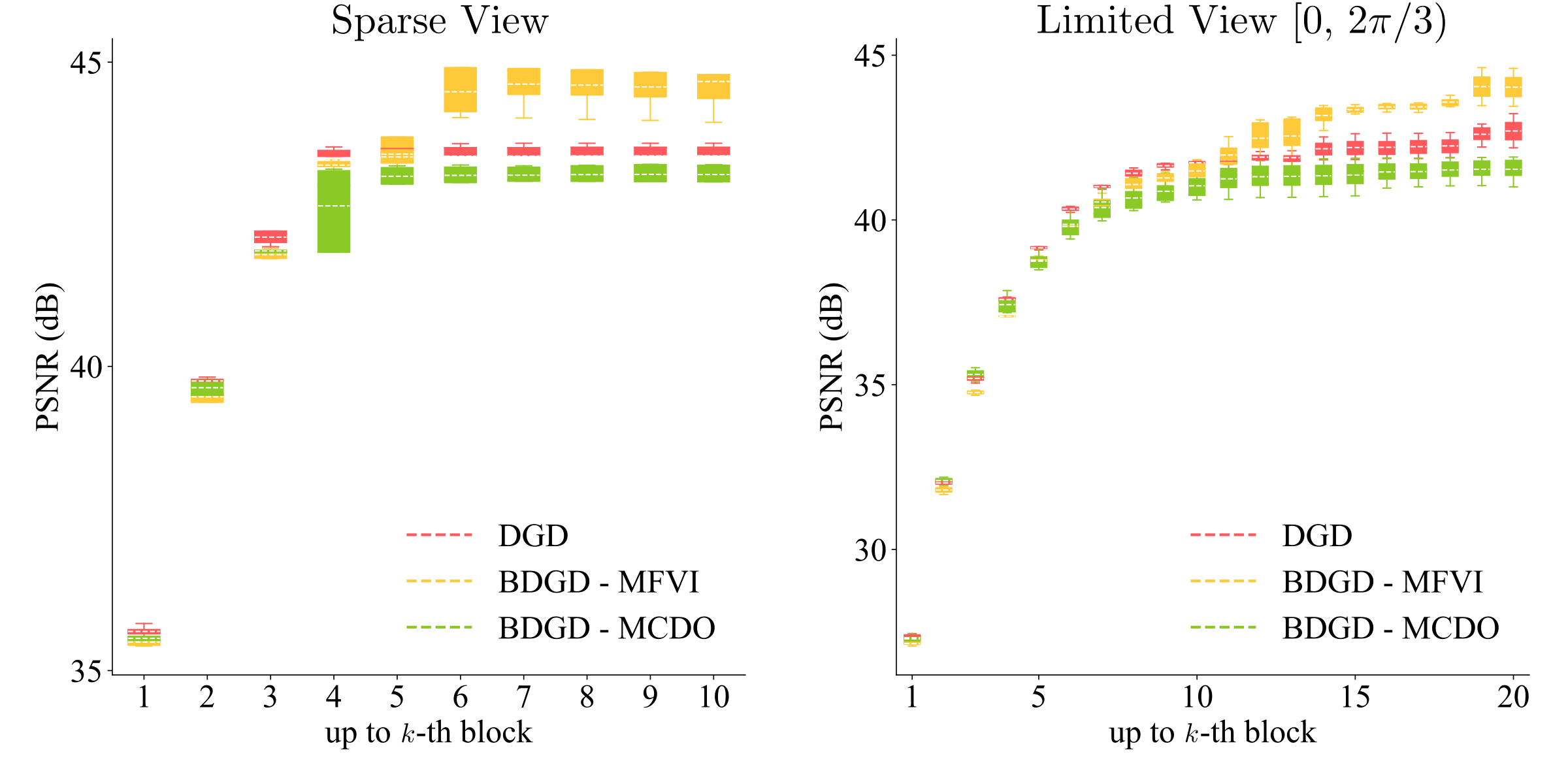
In Table I, we present numerical results for sparse view CT with 30 directions uniformly taken from 0 to $\pi$, computed with $K=10$ (further increasing the cascade’s depth does not lead to better reconstructions). Table I indicates that BDGD-MFVI outperforms all other methods on both test cases, with the only exception being LPD on the ellipses. In Fig. 2, we show the reconstructions of the SL phantom, and to shed insights into the working mechanisms of BDGD, we show the mean and pixel variance after the first, fifth, and tenth blocks. It is observed that both BDGD-MFVI and BDGD-MCDO show large pixel variance at $k=1$, which is reduced at $k=5$. However, BDGD-MFVI shows larger pixel variance at $k=10$ than at $k=5$, whereas BDGD-MCDO still presents low epistemic uncertainty. The boxplot in Fig. 3 (Left) shows the evolution of PSNR with the number $k$ of blocks. Interestingly, during the first few blocks, BDGD-MFVI and BDGD-MCDO perform comparably, but BDGD-MFVI allows further improvement with additional blocks.

In BDGD-MFVI there appear two distinct phases from a variance standpoint. In the first phase, i.e., the reconstruction phase, the method gradually improves the sample quality and reduces the overall uncertainty. For instance, Fig. 2 shows that BDGD-MFVI exhibits high variance up to the first block, i.e., the reconstructions disagree the most. As the method progresses up to the fifth block, the reconstruction shows reduced epistemic uncertainty. In the second phase, i.e., the fine-tuning phase, the method improves the sample quality and gradually reveals more uncertainty for fine details. That is, the greedy training strategy actually incrementally improves the reconstruction. Overall, BDGD-MFVI performs better than BDGD-MCDO, which, in terms of PSNR, behaves nearly identically to the deterministic counterpart (DGD) on the ellipses (we also fail to observe a fine-tuning phase), whereas on the SL phantom, BDGD-MCDO outperforms DGD, showing again the benefit of being Bayesian.

We show results for limited view $[0,2\pi/3)$, using $K=20$; see Table II for PSNR. As before, BDGD-MFVI outperforms other methods on both datasets in terms of PSNR. Fig. 4 shows the reconstruction of an ellipse phantom, along with the pixel variance for BDGD (for both MFVI and MCDO). In the phantom, a larger ellipse almost blends into the background, which is very challenging to reconstruct for all the methods under consideration. However, the presence of the ellipse is well captured by the variance in BDGD-MFVI. Thus, being Bayesian indeed allows a more thorough analysis of the reconstructed image. Note that the uncertainties by BDGD-MFVI capture far more detail about the ellipse edges than those by BDGD-MCDO, and thus are potentially more informative than the latter. Fig. 3 (Right) shows the boxplot of the evolution of PSNR with the number of blocks, which exhibits a similar behaviour to the sparse view case.

One of the serious issues with CT reconstructions is the introduction of artefacts due to insufficient information in the data. Thus, it is of significant interest to have indicators on such artefacts. Interestingly, BDGD can provide indicative information by allocating higher variances in related regions, cf. Fig. 5, which also includes a more challenging scenario, i.e., limited view $[0,\pi/3)$. In particular, as the view angle range decreases, the magnitude and significant areas of the variance increase, flaring up potential issues with the reconstruction in relevant regions.

A very similar phenomenon can be observed, in an even more striking way, in the out-of-distribution test data. In this test, we have added the text “ICPR 2020” in the ground truth phantom, following the work [20]. Having abnormal objects in the ellipses patterns, large uncertainty quantities now concentrate on the area around the text, indicating potentially serious issues in the region. This shows the benefit of conveying a notion of uncertainty in addition to a point estimate.

References

- [1] A. N. Tikhonov and V. Y. Arsenin, Solutions of Ill-posed Problems. V. H. Winston & Sons, Washington, D.C.: John Wiley & Sons, New York-Toronto, Ont.-London, 1977.
- [2] H. W. Engl, M. Hanke, and A. Neubauer, Regularization of Inverse Problems. Kluwer Academic, Dordrecht, 1996.
- [3] K. Ito and B. Jin, Inverse Problems: Tikhonov Theory and Algorithms. World Scientific Publishing Co. Pte. Ltd., Hackensack, NJ, 2015.
- [4] J. Sun, H. Li, Z. Xu, and Y. Yan, “Deep ADMM-Net for compressive sensing MRI,” in NIPS, 2016, pp. 10–18.
- [5] K. Hammernik, T. Klatzer, E. Kobler, M. P. Recht, D. K. Sodickson, T. Pock, and F. Knoll, “Learning a variational network for reconstruction of accelerated MRI data,” Mag. Reson. Med., vol. 79, no. 6, pp. 3055–3071, 2018.
- [6] H. Gupta, K. H. Jin, H. Q. Nguyen, M. T. McCann, and M. Unser, “CNN-based projected gradient descent for consistent CT image reconstruction,” IEEE Trans. Med. Imag., vol. 37, no. 6, pp. 1440–1453, 2018.
- [7] J. Adler and O. Öktem, “Learned primal-dual reconstruction,” IEEE Trans. Med. Imag., vol. 37, no. 6, pp. 1322–1332, 2018.
- [8] B. Zhu, J. Z. Liu, S. F. Cauley, B. R. Rosen, and M. S. Rosen, “Image reconstruction by domain-transform manifold learning,” Nature, vol. 555, pp. 487–492, 2018.
- [9] D. Ulyanov, A. Vedaldi, and V. Lempitsky, “Deep image prior,” in CVPR, June 2018.
- [10] S. Arridge, P. Maass, O. Öktem, and C.-B. Schönlieb, “Solving inverse problems using data-driven models,” Acta Numerica, vol. 28, pp. 1–174, 2019.
- [11] K. Zhang, W. Zuo, Y. Chen, D. Meng, and L. Zhang, “Beyond a Gaussian denoiser: Residual learning of deep CNN for image denoising,” IEEE Trans. Imag. Proc., vol. 26, no. 7, pp. 3142–3155, 2017.
- [12] C. Dong, C. C. Loy, K. He, and X. Tang, “Image super-resolution using deep convolutional networks,” IEEE Trans. Pattern Anal. Mach. Intel., vol. 38, no. 2, pp. 295–307, 2015.
- [13] C. M. Hyun, H. P. Kim, S. M. Lee, S. Lee, and J. K. Seo, “Deep learning for undersampled MRI reconstruction,” Phys. Med. Biol., vol. 63, no. 13, p. 135007, 2018.
- [14] Q. Yang, P. Yan, Y. Zhang, H. Yu, Y. Shi, X. Mou, M. K. Kalra, Y. Zhang, L. Sun, and G. Wang, “Low-dose CT image denoising using a generative adversarial network with Wasserstein distance and perceptual loss,” IEEE Trans. Med. Imag., vol. 37, no. 6, pp. 1348–1357, 2018.
- [15] A. Hauptmann, F. Lucka, M. Betcke, N. Huynh, J. Adler, B. Cox, P. Beard, S. Ourselin, and S. Arridge, “Model-based learning for accelerated, limited-view 3-D photoacoustic tomography,” IEEE Trans. Med. Imag., vol. 37, no. 6, pp. 1382–1393, 2018.
- [16] K. Gregor and Y. LeCun, “Learning fast approximations of sparse coding,” in ICML, 2010, pp. 1–8.
- [17] P. Putzky and M. Welling, “Recurrent inference machines for solving inverse problems,” arXiv:1706.04008, 2017.
- [18] V. Monga, Y. Li, and Y. C. Eldar, “Algorithm unrolling: Interpretable, efficient deep learning for signal and image processing,” arXiv:1912.10557, 2019.
- [19] G. Ongie, A. Jalal, R. G. Baraniuk, C. A. Metzler, A. G. Dimakis, and R. Willett, “Deep learning techniques for inverse problems in imaging,” IEEE J. Sel. Areas Inf. Theory, pp. 39 – 56 in press, 2020.
- [20] V. Antun, F. Renna, C. Poon, B. Adcock, and A. C. Hansen, “On instabilities of deep learning in image reconstruction and the potential costs of AI,” PNAS, 2020.
- [21] Y. Gal, “Uncertainty in Deep Learning,” Ph.D. dissertation, University of Cambridge, 2016.
- [22] J. Kaipio and E. Somersalo, Statistical and Computational Inverse Problems. Springer-Verlag, New York, 2005.
- [23] J. Adler and O. Öktem, “Deep Bayesian inversion,” arXiv:1811.05910, 2018.
- [24] C. Zhang and B. Jin, “Probabilistic residual learning for aleatoric uncertainty in image restoration,” arXiv:1908.01010, 2019.
- [25] A. Graves, “Practical variational inference for neural networks,” in NIPS, 2011, pp. 2348–2356.
- [26] C. Blundell, J. Cornebise, K. Kavukcuoglu, and D. Wierstra, “Weight uncertainty in neural networks,” arXiv:1505.05424, 2015.
- [27] D. Gamerman and H. F. Lopes, Markov Chain Monte Carlo: Stochastic Simulation for Bayesian Inference. CRC Press, 2006.
- [28] T. Papamarkou, J. Hinkle, M. Young, and D. Womble, “Challenges in Bayesian inference via Markov chain Monte Carlo for neural networks,” arXiv:1910.06539, 2019.
- [29] A. Repetti, M. Pereyra, and Y. Wiaux, “Scalable Bayesian uncertainty quantification in imaging inverse problems via convex optimization,” SIAM J. Imaging Sci., vol. 12, no. 1, pp. 87–118, 2019.
- [30] D. M. Blei, A. Kucukelbir, and J. D. McAuliffe, “Variational inference: A review for statisticians,” J. Amer. Stat Assoc., vol. 112, no. 518, pp. 859–877, 2017.
- [31] C. Zhang, J. Butepage, H. Kjellstrom, and S. Mandt, “Advances in variational inference,” IEEE Trans. Pattern Anal. Mach. Intell., vol. 41, no. 8, pp. 2008–2026, 2019.
- [32] K. Osawa, S. Swaroop, M. E. E. Khan, A. Jain, R. Eschenhagen, R. E. Turner, and R. Yokota, “Practical deep learning with Bayesian principles,” in NIPS, 2019.
- [33] S. Rossi, P. Michiardi, and M. Filippone, “Good initializations of variational bayes for deep models,” in ICML, 2019, pp. 5487–5497.
- [34] N. Srivastava, G. Hinton, A. Krizhevsky, I. Sutskever, and R. Salakhutdinov, “Dropout: a simple way to prevent neural networks from overfitting,” J. Mach. Learn. Res., vol. 15, no. 1, pp. 1929–1958, 2014.
- [35] Y. Gal and Z. Ghahramani, “Dropout as a Bayesian approximation: Representing model uncertainty in deep learning,” in ICML, 2016, pp. 1050–1059.
- [36] I. Osband, “Risk versus uncertainty in deep learning: Bayes, bootstrap and the dangers of dropout,” 2016.
- [37] A. Y. Foong, D. R. Burt, Y. Li, and R. E. Turner, “Pathologies of factorised Gaussian and MC dropout posteriors in Bayesian neural networks,” arXiv:1909.00719, 2019.
- [38] C. Riquelme, G. Tucker, and J. Snoek, “Deep Bayesian bandits showdown: An empirical comparison of Bayesian deep networks for Thompson sampling,” arXiv:1802.09127, 2018.
- [39] C. M. Bishop, Pattern Recognition and Machine Learning. Springer, 2006.
- [40] S. Kullback and R. A. Leibler, “On information and sufficiency,” Ann. Math. Statistics, vol. 22, pp. 79–86, 1951.
- [41] D. P. Kingma and M. Welling, “Auto-encoding variational Bayes,” arXiv:1312.6114, 2013.
- [42] D. P. Kingma, T. Salimans, and M. Welling, “Variational dropout and the local reparameterization trick,” in NIPS, 2015, pp. 2575–2583.
- [43] M. E. Khan, D. Nielsen, V. Tangkaratt, W. Lin, Y. Gal, and A. Srivastava, “Fast and scalable Bayesian deep learning by weight-perturbation in ADAM,” arXiv:1806.04854, 2018.
- [44] J. Hron, A. G. d. G. Matthews, and Z. Ghahramani, “Variational Bayesian dropout: pitfalls and fixes,” arXiv:1807.01969, 2018.
- [45] L. I. Rudin, S. Osher, and E. Fatemi, “Nonlinear total variation based noise removal algorithms,” 1992, vol. 60, no. 1-4, pp. 259–268.
- [46] J. Adler, H. Kohr, and O. Oktem, “Operator discretization library (odl),” Software available from https://github.com/odlgroup/odl, 2017.
- [47] W. Van Aarle, W. J. Palenstijn, J. Cant, E. Janssens, F. Bleichrodt, A. Dabravolski, J. De Beenhouwer, K. J. Batenburg, and J. Sijbers, “Fast and flexible X-ray tomography using the ASTRA toolbox,” Optics Expr., vol. 24, no. 22, pp. 25 129–25 147, 2016.