Anisotropic Neutron Stars Modelling: Constraints in Krori-Barua Spacetime

Very early in the study of pulsars it was realized that anisotropies inside the star can grow due to superfluidity [1, 2] (see [3] for a modern review) and solidification [4, 5, 6, 7]. An anisotropic core may also originate [8] from hyperons [9], quarks [10] as well as pion and kaon condensates [11, 12]. In addition, nuclear matter in a magnetic field becomes anisotropic, with different pressures in directions along and transverse to the field [13, 14]. The electromagnetic energy-momentum tensor is naturally anisotropic. Accounting for all these theoretical predictions it seems more realistic that pulsars contain an anisotropic core, rather than an ideally isotropic one.

The theory of anisotropic compact objects in General Relativity has been developing for half a century. Bowers & Liang [15] calculated the anisotropic generalization of Tolman-Oppenheimer-Volkov equation and generalized Bondi’s analysis [16]. An isotropic solution involves the emergence of a tangential pressure $p_{t}=p_{\theta}=p_{\phi}$ in the angular directions that is different than the radial pressure $p_{r}\neq p_{t}$. If the anisotropy parameter is positive $\Delta\equiv p_{t}-p_{r}>0$ an additional repulsive anisotropic force enhances stability, enabling more compact stable configurations to appear in the anisotropic than in the isotropic case [17]. It is in particular proposed [18, 19] that anisotropic compact stars may be arbitrarily compact up to compactness $C=2GM/Rc^{2}$ equal to one. Heintzmann & Hillebrandt [20] estimated the maximum mass of anisotropic compact stars $M_{\rm max}\sim 4M_{\odot}$ by use of semi-realistic equations of state. The Jeans stability criterion has been extended in the anisotropic case by Herrera & Santos [21].

A lot of anisotropic solutions and anisotropic compact star models have been proposed and studied [22, 23, 24, 25, 26, 27, 28, 29, 30, 31, 32]. Ivanov has calculated general bounds on the redshift for any anisotropic compact star in Ref. [33]. We will work here in a metric ansatz introduced by Krori & Barua [34]. Anisotropic compact star models in the Krori-Barua spacetime in General Relativity have been studied in Refs. [35, 36, 37, 38, 39, 40] and in modified theories of gravity in Refs. [41, 42, 43, 44, 45, 46, 47, 48, 49, 50, 51].

We will perform a general analysis of physical viability and stability of anisotropic solutions in KB-spacetime without preassuming an equation of state. We introduce dimensionless variables in which the KB-solutions can be parametrized with respect to the compactness. We impose general conditions for stability and physical consistency, which imply constraints on the maximum allowed compactness. We further use pulsars’ observational data of total mass and radius to estimate the boundary density of the core within our model and calculate the predicted mass-radius curve under a certain boundary condition.

To this end we have to use measurements of the mass and radius of pulsars, which are independent and do not rely on pre-assumptions regarding the equation of state in the core. We shall use six pulsars, members of low-mass X-ray binaries, which present thermonuclear bursts and therefore is possbile to get correlated $M-R$ constraints [52, 53]. More importantly we shall use data from additional two rotation-powered millisecond pulsars, PSR J0437-4715 and PSR J0030+0451, for which there exist reliable measurements of their radius independent from measurements of their mass and also not depending on assumptions regarding the equation of state [53, 54, 55, 56]. These two pulsars are special in that such measurements are as yet very rare. Both pulsars data are found to be consistent with the same boundary density which amazingly turns out to equal the nuclear saturation density that typically designates the boundary of the neutron core.

In addition, we shall use data regarding the recent gravitational-wave signals GW170817 [57, 58] and GW190814 [59]. We will finally supplement our analysis with data regarding quiescent low-mass X-ray binaries [60, 61] and pulsars presenting thermonuclear bursts [62].

In the next section we review KB-spacetime and introduce our dimensionless variables. In section 3 we perform the physics and stability analysis. In section 4 we discuss observational data and in the final section we discuss our conclusions.

A general spherically symmetric metric in General Relativity may be written in the spherical coordinates $(t,r,\theta,\phi)$ as

where $\alpha(r)$ and $\beta(r)$ are unknown functions of $r$. The spherically symmetric, anisotropic energy momentum tensor may be written as

where $\rho$, $p_{r}$, $p_{t}$ denote the mass density, the radial pressure and the tangential pressure, respectively. We denote $u^{\mu}$ the four-velocity and $\xi^{\mu}$ is the unit space-like vector in the radial direction. The energy-momentum tensor can always be brought in the diagonal form $T^{\mu}_{\nu}={\rm diag}(\rho c^{2},-p_{r},-p_{t},-p_{t})$.

Einstein equations give

where prime denotes derivative w.r.t the radial coordinate $r$.

Following Krori & Barua [34] we assume the following ansatz for the metric potentials

where however we use the dimensionless variable

and the star is assumed to be extended up to the radius $r=R$. The parameters $a_{0}$, $a_{1}$, $a_{2}$ in our ansatz are dimensionless and will be determined from the matching conditions on the boundary. The KB ansatz (6) ensures that the gravitational potentials and their derivatives are finite at the center.

We further introduce the characteristic density

which we use to scale the density and pressures, getting the dimensionless variables

Here $\Delta(r)=p_{t}-p_{r}$ is the anisotropic parameter of the star. Note that for a typical radius of neutron stars $R=10{\rm km}$ we get $\rho_{\star}=5.4\cdot 10^{14}{\rm gr/cm^{3}}$ that is twice the nuclear saturation density $\rho_{\rm sat}=2.7\cdot 10^{14}{\rm gr/cm^{3}}$. Using the dimensionless variables (9) and substituting (6) in the system (3)-(5) we get

The mass contained within a radius $r$ of the sphere is defined as

Substituting the density we get

where $M$ denotes the total mass of the star and $C$ is the compactness

We match the interior solution with the Schwartzschild solution at the boundary of the star $r=R$. In addition we assume that the radial pressure vanishes at the boundary. Our boundary conditions are therefore

By use of Eqs. (6), (11), the boundary conditions (17) give the dimensionless parameters $a_{0}$, $a_{1}$ and $a_{2}$ with respect to the compactness of the star as follows

Note also that since $C<1$ we get

Thus, we parametrized any neutron star model in KB-spacetime with respect to the compactness of the star. The quantities $\tilde{\rho}(x;C)$, $\tilde{p}_{r}(x;C)$, $\tilde{p}_{t}(x;C)$ are the same for stars with the same compactness $C$. In Figure 1 is evident that the equation of state $p_{r}=p_{r}(\rho)$, $p_{t}=p_{t}(\rho)$ is well fitted by a linear fit. In Figures 1, 1 we plot the slope of the fit with respect to compactness. It is evident that causality is violated for sufficiently high compactness. We discuss in detail the constraints imposed by requiring that the solution is stable and physical in the next section.

We impose the following reasonable physical requirements to a KB-spacetime (outlined in general very nicely in [63]).

1. i

   The gravitational potentials $\exp(\alpha(r))$, $\exp(\beta(r))$ and the physical quantities $\rho(r)$, $p_{r}(r)$, $p_{t}(r)$ should be well defined in the center as well as regular and singularity free throughout the interior of the star. These properties are directly implied by Eqs. (6), (10), (11), (12).

2. ii

   The anisotropy parameter should be positive throughout the whole interior of the star [64, 65]. Indeed, we have that

   $$e^{a_{2}x^{2}}-1-a_{2}x^{2}-a_{0}(a_{2}-a_{0})x^{4}=\sum_{n=3}^{\infty}\frac{1}{n!}(a_{2}x^{2})^{n}+\frac{1}{2}(a_{2}-a_{0})^{2}x^{4}+\frac{1}{2}a_{0}^{2}x^{4}>0.$$

   (20)

   From Eq. (13) follows directly that $\Delta>0$ for all $a_{0}$, $a_{2}$, $r$. It should also be vanishing in the center. Indeed, we have

   $$\tilde{p}_{r}(0)=\tilde{p}_{t}(0)=2a_{0}-a_{2}.$$

   (21)

3. iii

   The energy density, the radial and tangential pressures should be positive at the center. The energy density at the center is

   $$\tilde{\rho}(0)=3a_{2}>0.$$

   (22)

   It is positive also throughout the stellar interior. Indeed

   $$e^{a_{2}r^{2}}-1+2a_{2}r^{2}=1+a_{2}r^{2}+\sum_{n=2}^{\infty}\frac{1}{n!}(a_{2}r^{2})^{n}-1+2a_{2}r^{2}=\sum_{n=2}^{\infty}\frac{1}{n!}(a_{2}r^{2})^{n}+3a_{2}r^{2}>0$$

   (23)

   which, considering Eq. (10), implies $\rho>0$. Regarding the radial and tangential pressure from Eq. (18) we get

   $$a_{0}=a_{2}f(C),\quad{\rm where}\,f(C)\equiv\frac{1}{2}\frac{C}{(1-C)\ln(1-C)^{-1}}\,.$$

   (24)

   Since $C<1$ we have $f(C)>1/2$. This is straightforward because $f(0)=1/2$ and $df/dC>0$. Thus

   $$a_{0}>\frac{a_{2}}{2}.$$

   (25)

   from which it follows $p_{r}(0)>0$, $p_{t}(0)>0$ where the central pressures are given in (21). The radial pressure is positive also throughout the whole interior of the star since

   $$1-e^{a_{2}x^{2}}+2a_{0}x^{2}=\frac{(1-C)^{x^{2}}-(1-C)}{(1-C)^{x^{2}+1}}>0,$$

   (26)

   because $C<1$ and $x\leq 1$. Considering Eq. (11), it follows that $p_{r}>0$. Since the anisotropy parameter is positive, the tangential pressure is also positive throughout the interior of a star.

4. iv

   The density and the pressures should be decreasing functions of $r$. We have

   	$\displaystyle\tilde{\rho}{\,}^{\prime}$	$\displaystyle=2\frac{e^{-a_{2}x^{2}}}{x^{3}}\left(-e^{a_{2}x^{2}}+1+a_{2}x^{2}-2a_{2}^{2}x^{4}\right)\,,$		(27)
   	$\displaystyle\tilde{p}_{r}{}^{\prime}$	$\displaystyle=2\frac{e^{-a_{2}x^{2}}}{x^{3}}\left(e^{a_{2}x^{2}}-1-a_{2}x^{2}-2a_{0}a_{2}x^{4}\right)\,,$		(28)
   	$\displaystyle\tilde{p}_{t}{}^{\prime}$	$\displaystyle=2xe^{-a_{2}x^{2}}\left(a_{0}^{2}+a_{2}^{2}-3a_{0}a_{2}-a_{0}a_{2}(a_{0}-a_{2})x^{2}\right)\,,$		(29)

   where prime denotes derivative with respect to $x$. We have

   $$-e^{a_{2}x^{2}}+1+a_{2}x^{2}-2a_{2}^{2}x^{4}=-\sum_{n=2}^{\infty}\frac{1}{n!}(a_{2}x^{2})^{n}-2a_{2}^{2}x^{4}<0\,,$$

   (30)

   which, considering Eq. (27), implies $\rho^{\prime}<0$. Regarding now $p_{r}^{\prime}$, we have by use of (18) that on the boundary the derivative is negative

   $$e^{a_{2}}-1-a_{2}-2a_{0}a_{2}=\frac{C-\ln(1-C)^{-1}}{1-C}<0\Rightarrow p_{r}^{\prime}(x=1)<0\,.$$

   (31)

   Since we have proven that $p_{r}>0$, it is possible for $p_{r}$ to be increasing somewhere in the interval $x\in(0,1)$ if and only if there exists $x_{0}$ such that

   $$\tilde{p}_{r}^{\prime\prime}(x_{0})=0\Rightarrow 1-e^{a_{2}x_{0}^{2}}+2a_{0}x_{0}^{2}=-2a_{0}x_{0}^{2}\,.$$

   (32)

   However we have that

   $$\tilde{p}_{r}>0\Rightarrow 1-e^{a_{2}x^{2}}+2a_{0}x^{2}>0\,,\quad\forall x\in(0,1)$$

   (33)

   and thus Eq. (32) is impossible. Since $p_{r}$ is positive in the interval $x\in[0,1)$, vanishes in the boundary $x=1$, and has no inflection point in the interval $(0,1)$ it follows that it is a decreasing function in $[0,1]$. The case of tangential pressure is more involved because there do exist inflection points of $p_{t}$. This occurs at high compactness and at low distance from the center, as depicted in Figure 2. We calculate numerically that for $p_{t}$ being a monotonically decreasing function the compactness should satisfy that

   $$C<0.94\,.$$

   (34)

   

   

5. v

   We require that causality holds, namely that the speed of sound $v^{2}=\frac{dp}{d\rho}$ is lower than the speed of light

   $$0\leq v_{r}\leq c\,,\quad 0\leq v_{t}\leq c,.$$

   (35)

   The radial and transverse velocity of sound are

   	$\displaystyle v_{r}{}^{2}$	$\displaystyle=\frac{dp_{r}}{d\rho}=c^{2}\frac{1+a_{2}x^{2}+2a_{0}a_{2}x^{4}-e^{a_{2}x^{2}}}{e^{a_{2}x^{2}}-1-a_{2}x^{2}+2a_{2}{}^{2}x^{4}},$		(36)
   	$\displaystyle v_{t}{}^{2}$	$\displaystyle=\frac{dp_{t}}{d\rho}=c^{2}\frac{x^{4}(3a_{0}a_{2}-a_{0}a_{2}{}^{2}x^{2}+a_{0}{}^{2}a_{2}x^{2}-a_{2}{}^{2}-a_{0}{}^{2})}{e^{a_{2}x^{2}}-1-a_{2}x^{2}+2a_{2}{}^{2}x^{4}}\,.$		(37)

   We find numerically that the inequalities (35) impose constraints on maximum allowed compactness. The radial velocity imposes that $C<0.86$ and the tangential velocity that $C<0.87$, therefore causality is satisfied if

   $$C<0.86.$$

   (38)

   These results are also in accordance with the linear fit of Figure 1. The fact that causality is not satisfied for sufficiently high compactness is depicted in Figure 3.

   

   

6. vi

   We require stability against cracking which is satisfied if [66, 67]

   $$0<v_{r}{}^{2}-v_{t}{}^{2}<c^{2}\,.$$

   (39)

   This condition imposes an additional constraint on maximum allowed compactness

   $$C<0.78.$$

   (40)

   The fact that cracking stability is violated for sufficiently high compactness is depicted in Figure 4.

   

   

7. vii

   We require that the strong energy condition (SEC) [68, 63] holds

   $$\rho c^{2}-p_{r}-2p_{t}>0\,.$$

   (41)

   It places an additional constraint to the maximum allowed compactness, which we calculate numerically to be

   $$C\leq 0.715\,.$$

   (42)

   In Figure 5 is depicted that indeed for sufficiently high compactness, SEC is violated.

   

   

8. viii

   Our model satisfies the stability condition for the adiabatic index [69, 70]

   $$\Gamma\equiv\frac{\rho+p_{r}}{p_{r}}\frac{dp_{r}}{d\rho}>\frac{4}{3}.$$

   (43)

   The adiabatic index may be written as

   $$\Gamma(x;C)=\frac{2x^{2}(a_{0}+a_{2})(1+a_{2}x^{2}+2a_{0}a_{2}x^{4}-e^{a_{2}x^{2}})}{(1-e^{a_{2}x^{2}}+2a_{0}x^{2})(e^{a_{2}x^{2}}-1-a_{2}x^{2}+2a_{2}{}^{2}x^{4})}.$$

   (44)

   From inequalities (26), (30) it follows that $\Gamma>0$. We verify numerically that $\Gamma$ is a monotonically increasing function for all $C\in[0,1]$ and $x\in[0,1]$, with $a_{0}=a_{0}(C)$, $a_{2}=a_{2}(C)$ as in Eq. (18). This is depicted in Figure (6). We also have that

   $$\Gamma(x=0)=\frac{4}{5}\frac{(\frac{a_{0}}{a_{2}}+1)(2\frac{a_{0}}{a_{2}}+\frac{1}{2})}{2\frac{a_{0}}{a_{2}}-1}>\frac{7}{5}\left(1+\frac{2\sqrt{6}}{7}\right),$$

   (45)

   where $\frac{a_{0}}{a_{2}}>\frac{1}{2}$ as in (25). The inequality (45) follows from the monotonicity of the function

   $$h(z)=\frac{4}{5}\frac{(z+1)(2z+\frac{1}{2})}{2z-1}$$

   (46)

   in the interval $z>\frac{1}{2}$. The function $h(z)$ presents a minimum at $z_{\rm min}=\frac{1}{2}+\frac{\sqrt{6}}{4}$. It is $h(z_{\rm min})=\frac{7}{5}\left(1+\frac{2\sqrt{6}}{7}\right)$. It follows that $\Gamma>4/3$ for all $x$ and $C$ in the interval $[0,1]$.

   

To conclude, we find that conditions (i), (ii), (iii), (viii) are all satisfied by KB-spacetime for any compactness value. Conditions (iv), (v), (vi), (vii) impose constraints to compactness given by (34), (38), (40), (42), respectively. Combining these constraints we get that it should hold

for a stable, physical solution within a KB-spacetime.

Independent mass measurements of neutron stars are relatively easy. Their fast pulsation is ideal for timing measurements and since the pulsar is often a member of a binary system, this precise timing can be used to measure its orbital motion with astonishing precision [53]. On the other hand the independent radius measurement, depending on the thermal emmision of the stellar surface, is much more difficult.

Rotation-powered millisecond pulsars allow for the measurement of radius based on thermal emmision in soft X-rays [53, 54]. The mass of the pulsar can be measured independently by radio-timing measurements. There exist two such pulsars, PSR J0437-4715 (we shall call J0437) and PSR J0030+0451 (we shall call J0030), for which there exist very recent independent and reliable measurements from NICER [55, 56].

In addition to J0437 and J0030 we consider the gravitational-wave signals GW170817[57, 58] and GW190814 [59]. GW170817 was the first detection of coalescence of two neutron stars [57]. The subsequent analysis of LIGO/Virgo collaboration [58] constrained significantly the radii and masses of the two neutron stars. GW190814 was the first detection of an object within the mass-gap [59] with mass $M=2.6{\rm M}_{\odot}$. If this component is a neutron star and not a black hole the equation of state is further constrained.

We supplement our analysis with data regarding two quiescent low-mass X-ray binaries [60, 61] and six pulsars, members of low-mass X-ray binaries, that present thermonuclear X-ray bursts. For such pulsars it is possible to get correlated $M-R$ constraints [52, 53] independent from assumptions regarding the equation of state.

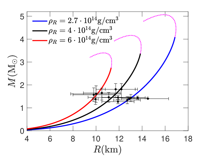
In Table 1 we see that the boundary density of all pulsars within a KB-spacetime lies in the range $(2.5-6.5)\cdot 10^{14}{\rm gr/cm^{3}}$. These values are consistent with a neutron core. All pulsars are consistent with a linear equation of state as already shown in Figure 1. The corresponding slope is depicted in the last column of Table 1.

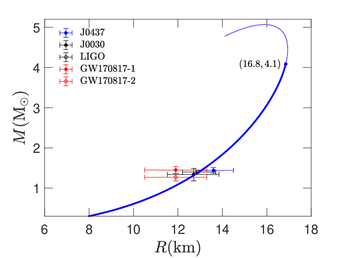
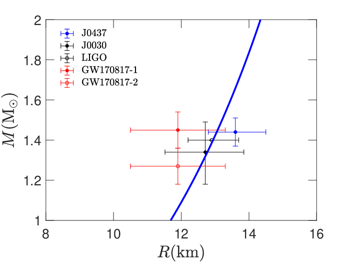
In Figure 7 is plotted the mass-radius curve with a certain boundary condition. It is evident that the most recent and reliable independent data from NICER and LIGO are consistent with the same boundary density which amazingly turns out to equal the nuclear saturation density $\rho_{\rm sat}=2.7\cdot 10^{14}{\rm gr/cm^{3}}$. This value perfectly describes a neutron core since typically it designates core’s boundary. Furthermore, anisotropies can grow down to this density. In Ref. [5] is argued that solidification occurs at the nuclear density $\rho_{\rm solid}=2.8\cdot 10^{14}{\rm gr/cm^{3}}$, and similar results are obtained in [73] which predict $\rho_{\rm solid}=3.7\cdot 10^{14}{\rm gr/cm^{3}}$. Even if solidification occurs at higher densities as predicted by other studies [6, 7], anisotropic superfluidity of nuclear matter appears at low densities such as $\rho=1.5\cdot 10^{14}{\rm gr/cm^{3}}$ [2].

The mass-radius curve with the boundary condition $\rho_{R}=\rho_{\rm sat}$, which fits well NICER and LIGO data, is depicted in Figure 8). We have calculated in previous section the maximum allowed compactness for a physical anisotropic core within a KB-spacetime to be $C_{\rm max}=0.71$. This limits the maximum mass to $M_{\rm max}=4.1M_{\odot}$ at $R=16.8{\rm km}$.

Our results does not exclude the possibility that the secondary component of GW190814 with mass $M=2.6{\rm M}_{\odot}$ is an anisotropic neutron star. The condition $C<0.71$ implies that it should have a radius $R>10.8{\rm km}$. The corresponding boundary density should be lower than $\rho_{R}<6.6\cdot 10^{14}{\rm g}/{\rm cm}^{3}$.

We parametrized any neutron star model in KB-spacetime with respect to the compactness of the star. This description is given by Eqs. (10), (11), (12), (18). Requiring that any KB-spacetime model of neutron stars is physical and the solution stable constraints the compactness to a maximum value

This is significantly more strict than the bound, $0.95$, obtained for general anisotropic stars in Ref. [33] and is in contrast to suggestions that anisotropic compact stars can be arbitrarily compact [18, 19].

The equations of state in a general KB-spacetime, depicted in Figure 1, are well fitted by a linear fit. A KB-spacetime fits observational data obtained from numerous pulsars of Table 1 with boundary density in the range $\rho_{R}\sim(2.5-6.5)\cdot 10^{14}{\rm gr/cm^{3}}$ consistent with an anisotropic neutron core. In Figure 7 we have calculated the mass-radius curves. An additional direct indication that KB-spacetime is realistic for anisotropic neutron stars is that the most recent data from NICER and LIGO are well fitted with boundary density which equals precisely the nuclear saturation density!

The mass-radius curve with boundary density that equals to the nuclear saturation density presents a mass maximum

when the bound (48) to compactness is also taken into account. This limits the maximum allowed mass for any consistent compact star model in KB-spacetime. This result is also in accordance with the estimated maximum mass in general spacetimes by Heintzmann & Hillebrandt [20], who use semi-realistic equations of state.

Our analysis predicts further that anisotropic neutron stars may populate partially the mass gap $(2.5-5)M_{\odot}$ regarding compact objects. An observation of a neutron star with $M>2.5M_{\odot}$ will be an indication it is composed of an anisotropic core. Especially, the possibility that the secondary component of the gravitational-wave signal GW190814 is a neutron star with an anisotropic core requires further investigation.

References

- [1] Gordon Baym, Christopher Pethick, and David Pines. Superfluidity in Neutron Stars. Nature, 224(5220):673–674, November 1969.
- [2] M. Hoffberg, et al. Anisotropic Superfluidity in Neutron Star Matter. Phys. Rev. Lett., 24(14):775–777, April 1970.
- [3] Armen Sedrakian and John W. Clark. Superfluidity in nuclear systems and neutron stars. European Physical Journal A, 55(9):167, September 2019.
- [4] P. W. Anderson and R. G. Palmer. Solidification Pressure of Nuclear and Neutron Star Matter. Nature Physical Science, 231(24):145–146, June 1971.
- [5] J. W. Clark and N. C. Chao. The Crystallization of Neutronic Matter. Nature Physical Science, 236(64):37–39, March 1972.
- [6] V. Canuto and S. M. Chitre. Solidification of Neutron Matter. Phys. Rev. Lett., 30(20):999–1002, May 1973.
- [7] Daniel Schiff. Crystallization Density of Cold Dense Neutron Matter. Nature Physical Science, 243(130):130–133, June 1973.
- [8] P. Haensel, A.Y. Potekhin, and D.G. Yakovlev. Neutron stars 1: Equation of state and structure, volume 326. Springer, New York, USA, 2007.
- [9] Shmuel Balberg and Nir Barnea. S-wave pairing of hyperons in dense matter. Phys. Rev. C, 57(1):409–416, January 1998.
- [10] D. Bailin and A. Love. Superfluidity and superconductivity in relativistic fermion systems. Phys. Rep. , 107(6):325–385, May 1984.
- [11] R. F. Sawyer. Condensed - Phase in Neutron-Star Matter. Phys. Rev. Lett., 29(6):382–385, August 1972.
- [12] T. Takatsuka and R. Tamagaki. Nucleon Superfluidity in Kaon-Condensed Neutron Stars. Progress of Theoretical Physics, 94(3):457–461, September 1995.
- [13] Efrain J. Ferrer, et al. Equation of state of a dense and magnetized fermion system. Phys. Rev. C, 82(6):065802, December 2010.
- [14] Efrain J. Ferrer and Aric Hackebill. Equation of State of a Magnetized Dense Neutron System. Universe, 5(5):104, May 2019.
- [15] Richard L. Bowers and E. P. T. Liang. Anisotropic Spheres in General Relativity. Astrophys. J., 188:657–665, 1974.
- [16] H. Bondi. Massive Spheres in General Relativity. Proceedings of the Royal Society of London Series A, 282(1390):303–317, November 1964.
- [17] B. V. Ivanov. Maximum bounds on the surface redshift of anisotropic stars. Phys. Rev. D, 65(10):104011, May 2002.
- [18] Marcelo Gleiser and Krsna Dev. Anisotropic stars: Exact solutions and stability. International Journal of Modern Physics D, 13(07):1389–1397, Aug 2004.
- [19] C G Böhmer and T Harko. Bounds on the basic physical parameters for anisotropic compact general relativistic objects. Classical and Quantum Gravity, 23(22):6479–6491, oct 2006.
- [20] H. Heintzmann and W. Hillebrandt. Neutron stars with an anisotropic equation of state: mass, redshift and stability. Astron. Astrophys., 38(1):51–55, January 1975.
- [21] L. Herrera and N. O. Santos. Jeans Mass for Anisotropic Matter. ApJ, 438:308, January 1995.
- [22] Selçuk Ş. Bayin. Anisotropic fluid spheres in general relativity. Phys. Rev. D, 26:1262–1274, Sep 1982.
- [23] L. Herrera, J. Ospino, and A. Di Prisco. All static spherically symmetric anisotropic solutions of einstein’s equations. Phys. Rev. D, 77:027502, Jan 2008.
- [24] S Thirukkanesh and S D Maharaj. Charged anisotropic matter with a linear equation of state. Classical and Quantum Gravity, 25(23):235001, nov 2008.
- [25] Ksh. Newton Singh, Piyali Bhar, and Neeraj Pant. Solutions of the Einstein’s field equations with anisotropic pressure compatible with cold star model. Astrophys. Space Sci., 361(10):339, October 2016.
- [26] S. K. Maurya, et al. Generalised model for anisotropic compact stars. The European Physical Journal C, 76(12), Dec 2016.
- [27] S. K. Maurya and M. Govender. Generating physically realizable stellar structures via embedding. The European Physical Journal C, 77(5), May 2017.
- [28] Gabino Estevez-Delgado and Joaquin Estevez-Delgado. On the effect of anisotropy on stellar models. European Physical Journal C, 78(8):673, August 2018.
- [29] Francisco Tello-Ortiz, et al. Anisotropic relativistic fluid spheres: an embedding class I approach. European Physical Journal C, 79(11):885, October 2019.
- [30] Shyam Das, Farook Rahaman, and Lipi Baskey. A new class of compact stellar model compatible with observational data. European Physical Journal C, 79(10):853, October 2019.
- [31] Joaquin Estevez-Delgado, et al. A possible representation for the neutron star PSR J0437-4715. European Physical Journal Plus, 134(12):600, December 2019.
- [32] Piyali Bhar. Anisotropic compact star model: a brief study via embedding. European Physical Journal C, 79(2):138, February 2019.
- [33] B. V. Ivanov. Maximum bounds on the surface redshift of anisotropic stars. Physical Review D, 65(10), Apr 2002.
- [34] K. D. Krori and J. Barua. A singularity-free solution for a charged fluid sphere in general relativity. Journal of Physics A Mathematical General, 8(4):508–511, April 1975.
- [35] Victor Varela, et al. Charged anisotropic matter with linear or nonlinear equation of state. Phys. Rev. D, 82:044052, Aug 2010.
- [36] Farook Rahaman, et al. Strange stars in Krori-Barua space-time. European Physical Journal C, 72:2071, July 2012.
- [37] Mehedi Kalam, et al. Central density dependent anisotropic compact stars. The European Physical Journal C, 73(4), Apr 2013.
- [38] Piyali Bhar. Strange quintessence star in Krori–Barua spacetime. Astrophys.& Space Sci., 356(2):365–373, 2015.
- [39] Piyali Bhar. Singularity-free anisotropic strange quintessence star. Astrophys. Space Sci., 356(2):309–318, April 2015.
- [40] Piyali Bhar, et al. Anisotropic charged fluids with chaplygin equation of state in ( 2 + 1 ) dimension. Astrophysics and Space Science, 360, 11 2015.
- [41] G. Abbas, Shahid Qaisar, and Abdul Jawad. Strange stars in f(T) gravity with MIT bag model. Astrophys. Space Sci., 359:17, October 2015.
- [42] M. Zubair, G. Abbas, and I. Noureen. Possible formation of compact stars in f(R,T) gravity. Astrophys. Space Sci., 361:8, January 2016.
- [43] M. Zubair and G. Abbas. Some interior models of compact stars in f(R) gravity. Astrophys. Space Sci., 361(10):342, October 2016.
- [44] M. Sharif and Arfa Waseem. Physical behavior of anisotropic compact stars inf(R,T,RT) gravity. Canadian Journal of Physics, 94(10):1024–1039, October 2016.
- [45] M. Ilyas, et al. Existence of relativistic structures in f(R,T) gravity. Astrophys. Space Sci., 362(12):237, December 2017.
- [46] Z. Yousaf, M. Zaeem-ul-Haq Bhatti, and M. Ilyas. Existence of compact structures in f( R, T) gravity. European Physical Journal C, 78(4):307, April 2018.
- [47] Ines G. Salako, Abdul Jawad, and Hooman Moradpour. Anisotropic compact stars in non-conservative theory of gravity. International Journal of Geometric Methods in Modern Physics, 15(6):1850093-595, January 2018.
- [48] M. Farasat Shamir and Adnan Malik. Behavior of Anisotropic Compact Stars in f(R, ) Gravity. Communications in Theoretical Physics, 71(5):599, May 2019.
- [49] Pameli Saha and Ujjal Debnath. Study of anisotropic compact stars with quintessence field and modified chaplygin gas in f( T) gravity. European Physical Journal C, 79(11):919, November 2019.
- [50] M. Farasat Shamir and I. Fayyaz. Charged anisotropic compact stars in Logarithmic-Corrected R2 gravity. International Journal of Modern Physics A, 35(4):2050013, February 2020.
- [51] M. Farasat Shamir and Iffat Fayyaz. Analysis of compact stars in logarithmic-corrected R2 gravity. Modern Physics Letters A, 35(2):1950354, January 2020.
- [52] F. Özel. Soft equations of state for neutron-star matter ruled out by EXO 0748 - 676. Nature, 441(7097):1115–1117, June 2006.
- [53] Feryal Özel and Paulo Freire. Masses, Radii, and the Equation of State of Neutron Stars. Ann. Rev. Astron. Astrophys., 54:401–440, September 2016.
- [54] Denis González-Caniulef, Sebastien Guillot, and Andreas Reisenegger. Neutron star radius measurement from the ultraviolet and soft X-ray thermal emission of PSR J0437-4715. MNRAS, 490(4):5848–5859, December 2019.
- [55] Slavko Bogdanov, et al. Constraining the Neutron Star Mass-Radius Relation and Dense Matter Equation of State with NICER. I. The Millisecond Pulsar X-Ray Data Set. ApJL, 887(1):L25, December 2019.
- [56] M. C. Miller, et al. PSR J0030+0451 Mass and Radius from NICER Data and Implications for the Properties of Neutron Star Matter. ApJL, 887(1):L24, December 2019.
- [57] B. P. Abbott et al. GW170817: Observation of Gravitational Waves from a Binary Neutron Star Inspiral. Phys. Rev. Lett., 119(16):161101, 2017.
- [58] B. P. Abbott, et al. Gw170817: Measurements of neutron star radii and equation of state. Phys. Rev. Lett., 121:161101, Oct 2018.
- [59] R. Abbott, et al. GW190814: Gravitational Waves from the Coalescence of a 23 Solar Mass Black Hole with a 2.6 Solar Mass Compact Object. ApJL, 896(2):L44, June 2020.
- [60] Craig O. Heinke, et al. A Hydrogen Atmosphere Spectral Model Applied to the Neutron Star X7 in the Globular Cluster 47 Tucanae. ApJ, 644(2):1090–1103, June 2006.
- [61] Natalie A. Webb and Didier Barret. Constraining the Equation of State of Supranuclear Dense Matter from XMM-Newton Observations of Neutron Stars in Globular Clusters. ApJ, 671(1):727–733, December 2007.
- [62] Feryal Özel, et al. The Dense Matter Equation of State from Neutron Star Radius and Mass Measurements. ApJ, 820(1):28, March 2016.
- [63] B. V. Ivanov. Analytical study of anisotropic compact star models. European Physical Journal C, 77(11):738, November 2017.
- [64] M. K. Mak and T. Harko. Can the galactic rotation curves be explained in brane world models? Phys. Rev. D, 70:024010, Jul 2004.
- [65] M. K. Mak and T. Harko. Quark stars admitting a one parameter group of conformal motions. Int. J. Mod. Phys., D13:149–156, 2004.
- [66] L. Herrera. Cracking of self-gravitating compact objects. Physics Letters A, 165(3):206 – 210, 1992.
- [67] H. Abreu, H. Hernández, and L. A. Núñez. Sound speeds, cracking and the stability of self-gravitating anisotropic compact objects. Classical and Quantum Gravity, 24(18):4631–4645, September 2007.
- [68] Charalampos A. Kolassis, Nilton O. Santos, and Dimitri Tsoubelis. Energy conditions for an imperfect fluid. Classical and Quantum Gravity, 5(10):1329–1338, October 1988.
- [69] R. Chan, L. Herrera, and N. O. Santos. Dynamical Instability for Shearing Viscous Collapse. MNRAS, 267:637, April 1994.
- [70] L. Herrera and N. O. Santos. Local anisotropy in self-gravitating systems. Phys. Rep. , 286:53–130, July 1997.
- [71] D. J. Reardon, et al. Timing analysis for 20 millisecond pulsars in the Parkes Pulsar Timing Array. MNRAS, 455(2):1751–1769, January 2016.
- [72] T. E. Riley, et al. A NICER View of PSR J0030+0451: Millisecond Pulsar Parameter Estimation. ApJL, 887(1):L21, December 2019.
- [73] V. Canuto. Equation of state at ultrahigh densities. Part 2. Ann. Rev. Astron. Astrophys., 13:335–380, January 1975.