Risk-Averse Equilibrium for Autonomous Vehicles in Stochastic Congestion Games
Abstract
The fast-growing market of autonomous vehicles, unmanned aerial vehicles, and fleets in general necessitates the design of smart and automatic navigation systems considering the stochastic latency along different paths in the traffic network. The longstanding shortest path problem in a deterministic network, whose counterpart in a congestion game setting is Wardrop equilibrium, has been studied extensively, but it is well known that finding the notion of an optimal path is challenging in a traffic network with stochastic arc delays. In this work, we propose three classes of risk-averse equilibria for an atomic stochastic congestion game in its general form where the arc delay distributions are load dependent and not necessarily independent of each other. The three classes are risk-averse equilibrium (RAE), mean-variance equilibrium (MVE), and conditional value at risk level equilibrium (CVaRαE) whose notions of risk-averse best responses are based on maximizing the probability of taking the shortest path, minimizing a linear combination of mean and variance of path delay, and minimizing the expected delay at a specified risky quantile of the delay distributions, respectively. We prove that for any finite stochastic atomic congestion game, the risk-averse, mean-variance, and CVaRα equilibria exist. We show that for risk-averse travelers, the Braess paradox may not occur to the extent presented originally since players do not necessarily travel along the shortest path in expectation, but they take the uncertainty of travel time into consideration as well. We show through some examples that the price of anarchy can be improved when players are risk-averse and travel according to one of the three classes of risk-averse equilibria rather than the Wardrop equilibrium.
keywords
Stochastic Congestion Games, Autonomous Vehicles, Risk-Aversion, Risk-Averse Equilibrium.1 Introduction
The intelligent transportation systems are growing faster than ever with the speedy emergence of autonomous vehicles, unmanned aerial vehicles, Amazon delivery robots, Uber/Lyft self-driving cars, and such. One of the principal components of such systems is the navigation system whose goal is to provide travelers with fast and reliable paths from their sources to destinations. In a fleet of vehicles, an equilibrium is achieved when no travelers have any incentives in a certain sense to change routes unilaterally. In the classical Wardrop equilibrium (Wardrop and Whitehead 1952, Wardrop 1952), travelers have incentives to change routes if they have an alternative route that has lower expected travel time. In other words, the optimality metric is based on minimizing the expected travel time in the Wardrop equilibrium. In the context of transportation though, collisions, weather conditions, road works, traffic signals, and varying traffic conditions can cause deviations in travel times (Ordóñez and Stier-Moses 2010). As a result, the path with the minimum expected travel time may not be reliable due to its high variability. Similarly, in the context of telecommunication networks, noise, signal degradation, interference, re-transmission, and malfunctioning equipment can cause variability in transmission time from source to destination (Ordóñez and Stier-Moses 2010). The empirical works by Abdel-Aty, Kitamura, and Jovanis 1995, Kazimi, Brownstone, and Gosh 2000, Lam and Small 2001, and Small 1999 also support the fact that taking travel time uncertainty into account is indeed an essential criterion in navigation systems.
As mentioned above, minimizing the expected travel time is inadequate in scenarios involving risk due to variability of travel times. In order to address this issue, we study a richer class of congestion games called stochastic congestion games in an atomic setting, where the travel times along different arcs of the network are random variables that are not necessarily independent of each other. In this framework, we introduce probability statements regarding the risk-averse best response of a traveler given the choice of the rest of travelers in the network. We propose three classes of risk-averse equilibria for stochastic congestion games: risk-averse equilibrium (RAE), mean-variance equilibrium (MVE), and conditional value at risk level equilibrium (CVaRαE), whose notions of risk-averse best responses are based on maximizing the probability of traveling along the shortest path (also known as Risk-Averse Best Action Decision with Incomplete Information (R-ABADI)), minimizing a linear combination of mean and variance of path delay, and minimizing the expected delay at a specified risky quantile of the delay distributions, respectively. We prove that the risk-averse, mean-variance, and CVaRα equilibria exist for any finite stochastic atomic congestion game. Note that two equilibria similar to the mean-variance and CVaR equilibria exist in the literature and are discussed in the related work section, but the probability distributions of travel times are load independent or link delays are considered to be independent in the literature, which is not the case in this article. It is noteworthy that most studies on stochastic congestion games make use of simplifying assumptions such as considering the arc delay distributions to be independent of their loads or adding independent and identically distributed errors to nominal delays of arcs neglecting their differences. In the Braess paradox (Braess 1968, Murchland 1970), which is known to be a counterintuitive example rather than a paradox, the risk-neutral/selfish travelers select the shortest path in expected travel time, which maximizes the social delay/cost incurred by the whole society. Although the focus of this article is not on deriving bounds on price of anarchy, we study the Braess paradox in a stochastic setting under the three proposed risk-averse equilibria and show that the risk-averse behavior of travelers results in improving the social delay/cost incurred by the society; and as a result, the price of anarchy is improved if travelers are risk-averse. As the result, the Braess paradox may not occur to the extent presented originally if travelers are risk-averse. Furthermore, we study the Pigou network (Pigou 1920) in a stochastic setting and observe that the price of anarchy is also improved if travelers are risk-averse in the senses discussed above. Note that the Pigou networks are prevalent in traffic/telecommunication networks. Hence, providing travelers with risk-averse navigation can decrease the social delay/cost in the real world applications.
The article is structured in the following way. The related work is discussed in Section 2. The stochastic congestion game is formally defined in Section 3. The three proposed classes of equilibria, i.e. risk-averse, mean-variance, and CVaRα equilibria, are presented in Section 4 and their existences in any finite stochastic congestion game are proven; detailed proofs can be found in the Appendix. Numerical results including the study of the Pigou and Braess networks as well as notes for practitioners are provided in Section 5. Finally, conclusions and discussion of opportunities for future work are provided in Section 6.
2 Related Work
In this section, the literature on navigation for both deterministic and stochastic networks is presented first, then the literature on deterministic and stochastic congestion games is discussed in details. The main focus of the literature review is to motivate the necessity of risk-averse algorithms for navigation and congestion games in a stochastic setting.
The problem of finding the shortest path in a transportation/telecommunication traffic network is one of the main parts of the in-vehicle navigation systems. This problem has been studied well in deterministic networks resulting in many efficient algorithms, e.g., the algorithms developed by Dijkstra 1959, and Dreyfus 1969; also see (Schrijver 2012, Fu, Sun, and Rilett 2006, Dial 1969, Tarjan 1983, Lawler 1976, Pierce 1975, Orda and Rom 1990, Kaufman and Smith 1993, Hall 1993, Chabini 1997), and (Hosseini et al. 2017). Although finding the shortest path problem is well understood in deterministic networks, the definition of an optimal path and how to identify such a path is more challenging in the stochastic version of the problem. There have been multiple approaches to define the optimal path in stochastic networks as summarized below. The least expected travel time is studied by Loui 1983 and is equivalent to the deterministic case from a computational point of view. The path with the least expected time may be sub-optimal for risk-averse travelers due to its high variability and uncertainty; as the result, the probability distributions of link travel times need to be considered explicitly to find the most reliable path. In this manner, Frank 1969 proposed the optimal path to be the one that maximizes the probability of realizing a travel time that less than a threshold, Sigal, Pritsker, and Solberg 1980 proposed the optimal path to be the one that maximizes the probability of realizing the shortest time, and Chen and Ji 2005 proposed the optimal path to be the one with minimum travel time budget required to meet a travel time reliability constraint. For more variants of the mentioned algorithms, refer to (Nie and Fan 2006, Nie and Wu 2009, Zeng et al. 2015, Xing and Zhou 2011, Howard 2012, Hall 1986, Fu and Rilett 1998, Waller and Ziliaskopoulos 2002, Miller-Hooks and Mahmassani 2000, Mirchandani et al. 1986, Mirchandani 1976, Murthy and Sarkar 1996, Fan 2003, Xiao and Lo 2013, Bell 2009, Chen, Bell, and Bogenberger 2010), and (Lo, Luo, and Siu 2006).
In the context of route selection in a fleet of vehicles, a game emerges between all travelers where the action of each traveler affects the travel time of the other travelers, which creates a competitive situation forcing travelers to strategize their decisions. In a deterministic network, the mentioned game is formalized by Wardrop and Whitehead 1952, Neumann 1928, Von Neumann and Morgenstern 1947, and Nash et al. 1950. However, it is not realistic to consider the link delays to be known prior to making a decision due to external factors that make the travel times uncertain. In order to put this in perspective, several approaches have been adopted by researchers to capture the stochastic behavior of the traffic networks. For example, Harsanyi 1967, Harsanyi 1968 proposed Bayesian games that consider the incomplete information of payoffs, Ordóñez and Stier-Moses 2010 modeled the risk-averse behavior of travelers by padding the expected travel time along paths with a safety margin, Watling 2006 proposed an equilibrium based on the optimality measure of minimizing the probability of being late or maximizing the probability of being on time, Szeto, O’Brien, and O’Mahony 2006 associated a cost with the travel time uncertainty based on travelers’ risk-averse behavior, Chen and Zhou 2010 proposed an equilibrium based on the optimality measure of minimizing the conditional expectation of travel time beyond a travel time budget, and Bell and Cassir 2002 proposed to play out all possible scenarios before making a choice. For more details in the context of traffic networks, we refer readers to (Aashtiani and Magnanti 1981, Aghassi and Bertsimas 2006, Altman et al. 2006, Hayashi, Yamashita, and Fukushima 2005, Mirchandani and Soroush 1987, Nie 2011, Connors and Sumalee 2009, Schmöcker et al. 2009, Fonzone et al. 2012, Angelidakis, Fotakis, and Lianeas 2013, Nikolova and Stier-Moses 2011, Nikolova and Stier-Moses 2015), and (Correa, Hoeksma, and Schröder 2019).
3 Problem Statement
Consider a directed graph (network) with a node set and directed link (edge) set with cardinality , where the pair indicates a directed link from node to node in the directed graph. Denote the set of source-destination (SD) pairs with , where for the SD pair , , the set of simple directed paths from to in is denoted by , and let be the number of players (travelers, vehicles, or data packages) associated with source-destination . Let be the set of all paths. A feasible assignment allocates a non-negative number of players to every path such that for all . As a result, the number of players along link denoted by is given by .
The latency (delay or travel time) along link is load-dependent which is denoted by the non-negative continuous random variable with marginal probability density function (pdf) and mean . Note that the number of players along an edge is determined by an assignment , so , , and can be used instead of , , and , respectively. Furthermore, the latency along links of the graph can be dependent, in which case, the joint pdf of latency over all links is denoted by , which can be denoted as . Given the link latency defined above, the nominal latency of player along path under a given assignment is simply with pdf and mean .
The stochastic congestion game consists of players (travelers), where player is associated with the corresponding source-destination pair . As a result, is the set of possible pure strategies (actions or paths) for player . The pure strategy profile of all players is denoted by , where , that fully specifies all actions in the game. The set of all pure strategy profiles is the Cartesian product of pure strategy sets of all players which is denoted by . Let be the pure strategies of all players except player , so . Given the pure strategy profile , the number of players on a path is given by , and the number of players on a link is given by . Let show the number of players on all paths which is fully determined by the pure strategy . As a result, given the pure strategy profile , the latency of player by choosing the path is the random variable with pdf and mean . For simplicity, instead of using , , and , we use , , and , respectively.
The mixed strategy of player is denoted by , where is the set of all probability distributions over the set of pure strategies , and is the probability that player selects path . The mixed strategy profile of all players is denoted by , where . The set of all mixed strategy profiles is the Cartesian product of mixed strategy sets of all players which is denoted by . Let be the mixed strategies of all players except player , so . The latency of player by selecting path when the other players select paths according to a mixed strategy is denoted by the random variable that has the following pdf using the law of total probability:
| (1) |
where and is the corresponding strategy of player in , and the mean of the random variable is given as
| (2) |
The expected average delay (latency) incurred by the players in the stochastic congestion game under the pure strategy profile , also known as the social cost or social delay in this context, is denoted by . The social delay under the mixed strategy is , where and is the corresponding strategy of player in . The (pure) optimal load assignment denoted by minimizes social delay among all possible (pure) load assignments which might be in contrast with the selfish behavior of players. The (pure) price of anarchy (PoA) of a congestion game is the maximum ratio over all equilibria of the game. Throughout the article, we follow the convention that means that is less than or equal to all elements of the vector .
4 Risk-Averse Equilibrium for Stochastic Congestion Games
In the following sub-section, illustrative examples are provided with analysis of their equilibria in classic and risk-averse frameworks which motivate the novel risk-averse approach for stochastic congestion games presented in this article.
4.1 Illustrative Examples
The Pigou network (Pigou 2013) is one of the simplest networks studied in congestion games. We first use the Pigou network to clearly state the motivation of the current work in the first example. We then study the more controversial network used by Braess 1968 in the famous Braess’s paradox in the second example. The two examples below set grounding for the risk-averse equilibrium for congestion games proposed in this article.
Example 4.1
Consider the Pigou network with two parallel links between source and destination as shown in Figure 1. There are players (vehicles or data packages) to travel from source to destination. The top and bottom links are labeled as and with loads and , respectively. The travel times on links and are respectively independent random variables and with expected values and and pdfs
where and are constants for which each of the two distributions integrate to one and is the indicator function.

The well-known Wardrop equilibrium (Wardrop 1952, Wardrop and Whitehead 1952), also Nash equilibrium (von Neumann and Morgenstern 1947), for the Pigou network in Example 4.1 is that all the players travel along the top link since it is the weakly dominant strategy for any player as the expected latency incurred along the top link is always less than or equal to the expected latency incurred along the bottom link, . As a result, the Wardrop equilibrium for Pigou network is with social delay . However, although the expected latency along the top link is less than or equal to that of the bottom link, , the variance of travel time along the top link at full capacity is larger than that along the bottom link, which increases the risk and uncertainty of traveling along the top link (Yekkehkhany, Murray, and Nagi 2020, Yekkehkhany et al. 2020, Yekkehkhany et al. 2019). In fact, the bottom link with higher expected travel time is more likely to have a lower delay than the top link at full capacity, i.e., . As a result, a risk-averse player selects the bottom link for commute when the top link is at full capacity, especially if it is a one-time trip. We will also shown later, the risk-averse behavior of players decreases social delay for this example. As an example, consider a traveler who wants to go from hotel to airport who has two options for this trip: taking the highway that has lower expected travel time, but is more likely to get congested due to traffic jams and crashes (top link in Pigou network), or taking the urban streets with a higher expected travel time and lower congestion (the bottom link in Pigou network). A risk-neutral player travels along the top link with lower expected latency, but a risk-averse player travels along the bottom link to assure not to incur a long delay and miss the flight. Even in everyday commutes between home and work, the expected delay over many days may not be a desirable objective to minimize. No-one desires to arrive early to work some days but late on others, and to be penalized accordingly. The Braess network, studied in the next example, further enforces the fact that minimizing the expected delay is not desirable for risk-averse players.

Example 4.2
Consider the Braess network depicted in Figure 2. There are players (vehicles or data packages) to travel from source to destination. Other than the source and destination, there are two nodes and in the network. The directed links , , , , and are referred to as links , , , , and with loads , , , , and , respectively. The travel times on links , , , , and are respectively independent random variables , , , , and with expected values , , , , and and pdfs
where and are constants for which the distributions integrate to one, is the indicator function, and . There are three paths from source to destination, , , and , that are referred to as paths , and with loads , and , respectively, where the difference between links and paths should be clear from the context. Note that the link loads are related to path loads as , , , , and , and the delays along paths are related to link delays as , , and .
The Wardrop (Nash) equilibrium for the Braess network in Example 4.2 is that all the players travel along path since it is the weakly dominant path for any player as the expected latency incurred along path is always less than or equal to the expected latency incurred along the other two paths and ,
As a result, the Wardrop equilibrium for Braess network is with social delay . However, although path has latency less than or equal to that of paths and , , the variance of travel time along path at full capacity is larger than that along paths and , which increases the risk and uncertainty of traveling along path . In fact, path (or ) with higher expected travel time is more likely to have a lower delay than the rest of the paths, i.e., . As a result, a risk-averse player selects paths or for commute when path is at full capacity, and as is shown later, the risk-averse behavior of players decreases social delay for this example.
4.2 Risk-Averse Equilibrium
In the classical Wardrop (Nash) equilibrium, the best response of player to the mixed strategy of the other players is defined as the set
In other words, the best response for player given is defined as the path that minimizes the expected travel time. However, motivated by Examples 4.1 and 4.2, the path with minimum expected latency may have a high volatility as well that causes risky scenarios for travelers. As a result, the classical Wardrop (Nash) equilibrium that ignores the distribution of path latency except for taking the expected latency into account, that does not carry any information about variance and the shape of the distribution, falls short in addressing risk-averse behavior of players. In this article, motivated by Examples 4.1 and 4.2, we propose a Risk-Averse Best Action Decision with Incomplete Information (R-ABADI) of a player to the strategy of the other players in a stochastic congestion game as follows.
Definition 4.3
Given the mixed strategy profile of players , the set of mixed strategy risk-averse best responses of player is the set of all probability distributions over the set
| (3) |
where what we mean by being less than or equal to when is that is less than or equal to for all ; otherwise, if , player only has a single option that can be played. The same randomness on the action of players is considered in for all . Given the mixed strategy of players , the risk-averse best response set of player ’s strategies is denoted by , which is in general a set-valued function.
The risk-averse equilibrium for stochastic congestion games is defined as follows.
Definition 4.4
A strategy profile is a risk-averse equilibrium if and only if for all .
The following theorem proves the existence of a risk-averse equilibrium for any stochastic congestion game with finite number of players and pure strategy sets for all with finite cardinality.
Theorem 4.5
For any finite -player stochastic congestion game, a risk-averse equilibrium exists.
As a direct result of Definitions 4.3 and 4.4, the pure strategy risk-averse best response and pure strategy risk-averse equilibrium are defined as follows. The pure strategy risk-averse best response of player to the pure strategy of players is the set
| (4) |
Given the pure strategy of players , the risk-averse best response set of player in Equation (4) is denoted by (overloading notation, is used for both pure and mixed strategy risk-averse best responses). As a result, a pure strategy profile is a pure strategy risk-averse equilibrium if and only if for all .
Strict dominance in the classical Wardrop (Nash) equilibrium is defined as follows. A pure strategy of player strictly dominates a second pure strategy of the player if
The solution concept of iterated elimination of strictly dominated strategies can also be applied to the risk-averse equilibrium using the following definition.
Definition 4.6
A pure strategy of player strictly dominates a second pure strategy of the player in the risk-averse equilibrium if
| (5) |
Consider path strictly dominates path for player ; then, for any
| (6) | ||||
where is true by the law of total probability, and is the corresponding strategy of player in , and is followed by Equation (5) in Definition 4.6. By Equation (6) and Equation (3) in Definition 4.3, a strictly dominated pure strategy cannot be a best response to any mixed strategy profile , so it can be removed from the set of strategies of player .
In order to find the risk-averse equilibrium for a stochastic congestion game, we use support enumeration. For example, hypothesize that is the support of a risk-averse equilibrium, where is the set of pure strategies of player that are played with non-zero probability and for indicates the probability mass function on the support. At equilibrium, player should be indifferent between strategies in the set , has no incentive to deviate to the rest of strategies in the set , and the probability mass function over the support should add to one. As a result, if there is a risk-averse equilibrium with the mentioned support, it is the solution of the following set of equations for :
| (7) |
As mentioned earlier in Equation (6), using the law of total probability, we have
| (8) | ||||
where is the -th element of an -dimensional vector called . Construct a risk-averse probability tensor of rank where forms the -th dimension of the tensor. Let the element associated with in the tensor be the vector . Equations (7) and (8) along with the definition of the risk-averse probability tensor provide us with an alternative approach for deriving the risk-averse equilibrium, which is to find the Wardrop (Nash) equilibrium on the risk-averse probability tensor.
The mean-variance (MV) and conditional value at risk level (CVaRα) methods are two well-known frameworks to consider risk in statistics. In the next two sub-sections, two new risk-averse equilibria based on these two concepts are proposed.
4.3 Mean-Variance Equilibrium
As seen in Examples 4.1 and 4.2, the high variance of paths with lower expected travel time can result in uncertainty and impose high latency for travelers. The mean-variance framework in statistics addresses this issue by keeping a balance between low latency and low variance. Applying this method to the proposed stochastic congestion game setting, the mean-variance best response and mean-variance equilibrium are defined as follows.
Definition 4.7
Given the mixed strategy profile of players , the set of mixed strategy mean-variance best responses of player is the set of all probability distributions over the set
| (9) |
where the variance can be calculated using the pdf of provided in Equation (1) and is a hyper-parameter capturing the absolute risk tolerance. Given the mixed strategy of players , the mean-variance best response set of player ’s strategies is denoted by , which is in general a set-valued function.
Definition 4.8
A strategy profile is a mean-variance equilibrium if and only if for all .
The existence of the mean-variance equilibrium is discussed in the following theorem.
Theorem 4.9
For any finite -player stochastic congestion game, a mean-variance equilibrium exists.
The pure strategy mean-variance best response of player to the pure strategy of players is the set
| (10) |
where . Given the pure strategy of players , the mean-variance best response set of player in Equation (10) is denoted by (overloading notation, is used for both pure and mixed strategy mean-variance best responses). As a result, a pure strategy profile is a pure strategy mean-variance equilibrium if and only if for all . The strict dominance concept is straightforward among pure strategy profiles in mean-variance equilibrium that is defined as follows. A pure strategy of player strictly dominates a second pure strategy of the player in pure strategy mean-variance equilibrium if
| (11) |
However, due to the fact that variance is not a linear operator, strict dominance may not be derived from Equation (11) for mixed strategy mean-variance equilibrium as described below.
| (12) | ||||
where is true by the definition of variance, is followed by Equation (2), is derived by expanding the second term, and is true by combining the summation over and factoring . As can be seen in Equation (12), since variance is a non-linear operator, it is not clear whether Equation (11) can result in for all . As a result, use of strict dominance in the mixed strategy mean-variance equilibrium is not advised. In certain circumstances though, we can propose conditions for strict dominance; e.g., when for all and for all which is discussed in the following definition or when for all and for all .
Definition 4.10
If for all and for all , pure strategy of player strictly dominates a second pure strategy of the player in the mean-variance equilibrium if
| (13) |
and
| (14) |
Consider that path strictly dominates path for player as defined in Definition 4.10; then, using Equation (13), for any ,
| (15) |
Note that for all , for all , and for all as a result of for all and for all . Hence, using the fact that the function is increasing for , for any we have
| (16) |
On the other hand, using Equation (14), we have
| (17) | ||||
In order to find the mean-variance equilibrium for a stochastic congestion game, we use support enumeration. For example, hypothesize to be the support of a mean-variance equilibrium, where is the set of pure strategies of player that are played with non-zero probability and for indicates the probability mass function on the support. At equilibrium, player should be indifferent between strategies in the set , has no incentive to deviate to the rest of strategies in the set , and the probability mass function over the support should add to one. As a result, if there is a mean-variance equilibrium with the mentioned support, it is the solution of the following set of equations for :
| (18) |
4.4 CVaRα Equilibrium
The conditional value at risk level (CVaRα) is another framework in statistics to measure risk and to address the risk-averse behavior. Applying this method to the proposed stochastic congestion game setting, the CVaRα best response and CVaRα equilibrium are defined below.
Definition 4.11
Given the mixed strategy profile of players , the set of mixed strategy CVaRα best responses of player is the set of all probability distributions over the set
| (19) |
where is a constant derived by solving the equality and the constant is a hyper-parameter depicting the risk level. Given the mixed strategy of players , the CVaRα best response set of player ’s strategies is denoted by , which is in general a set-valued function.
Definition 4.12
A strategy profile is a CVaRα equilibrium if and only if for all .
The existence of the CVaRα equilibrium is discussed in the following theorem.
Theorem 4.13
For any finite -player stochastic congestion game, a CVaRα equilibrium exists.
The pure strategy CVaRα best response of player to the pure strategy of players is the set
| (20) |
where is a constant derived by solving the equality and the constant is the hyper-parameter depicting risk level. Given the pure strategy of players , the CVaRα best response set of player in Equation (20) is denoted by (overloading notation, is used for both pure and mixed strategy CVaRα best responses). As a result, a pure strategy profile is a pure strategy CVaRα equilibrium if and only if for all . A pure strategy of player strictly dominates a second pure strategy of the player in pure strategy CVaRα equilibrium if
| (21) |
where and are constants derived by solving and , and the constant is the risk level hyper-parameter. However, similar to the mean-variance equilibrium, strict dominance may not be derived from Equation (21) for mixed strategy CVaRα equilibrium as described below. Using Equation (1) and , the distribution of the random variable is
| (22) |
As a result,
| (23) | ||||
where is true by using the pdf of the corresponding random variable in Equation (22) and switching the order of summation and integral and is true by multiplying and dividing by the term . As can be seen in Equation (23), it is not clear whether Equation (21) can result in for all . As a result, use of strict dominance in the mixed strategy CVaRα equilibrium is not advised due to its complication.
In order to find the CVaRα equilibrium for a stochastic congestion game, we use support enumeration. For example, hypothesize to be the support of a CVaRα equilibrium, where is the set of pure strategies of player that are played with non-zero probability and for indicates the probability mass function on the support. At equilibrium, player should be indifferent between strategies in the set , has no incentive to deviate to the rest of strategies in the set , and the probability mass function over the support should add to one. As a result, if there is a CVaRα equilibrium with the mentioned support, it is the solution of the following set of equations for :
| (24) |
Remark 4.14
It is noteworthy that the polynomial terms in Equation (7) for the risk-averse equilibrium are of degree while the polynomial terms in Equation (18) for the mean-variance equilibrium are of degree for number of players. On the other hand, it is more complicated to solve for Equation (24) as the top quantile of distributions should be calculated.
5 Numerical Results
The risk-averse, mean-variance, and CVaRα equilibria are numerically analyzed for Examples 4.1 and 4.2 in this section. The price of anarchy for each of the mentioned equilibria is calculated as well. In the end, extra examples are presented to shed light on the corner cases of each one of the equilibria and to provide insight on how to tackle such circumstances.
In order to find any of the three types of pure equilibria for the Pigou network in Example 4.1 with players, hypothesize that players choose link and players choose link and check whether any players has any incentive in the corresponding sense of the equilibrium of the interest to change route, given the pure strategy of the other players. If none of the players has any incentive to change route given the pure strategy of the rest of players, is a pure equilibrium, where denotes that players select link and players select link . By varying from zero to and taking the above procedure, the pure equilibrium is found if any exists. Given a fixed number of players that choose link , it is obvious that they all have the same incentive to change to link or stay in link , and all of the players have the same incentive to change to link or stay in link . As a result, if a specific player out of the players has no incentive to switch to link given the pure strategy of the other players, and a specific player out of the players has no incentive to switch to link given the pure strategy of the other players, is a pure equilibrium. In other words, is a pure risk-averse equilibrium if
| (25) |
where the first inequality is true since each player has two options, link and link , so , and since random variables are continuous we have , which results in . The second inequality is true due to a similar reasoning. By varying from zero to , if Equation (25) holds for , it is a pure risk-averse equilibrium.
Similar to the above approach, is a pure mean-variance equilibrium if
| (26) |
Again, by varying from zero to , if Equation (26) holds for , it is a pure mean-variance equilibrium. Similarly, is a pure CVaRα equilibrium if
| (27) |
where . By varying from zero to , if Equation (27) holds for , it is a pure CVaRα equilibrium.
Note that the equilibrium in the Pigou network in Example 4.1 is characterized by , since can be derived given . The pure risk-averse, mean-variance (), and CVaRα () equilibria are found for the mentioned Pigou network and the proportion of players who select link , i.e., , is depicted in Figure 3 for different values of . Under the Nash equilibrium, no matter what the probability distributions of latency over links look like, all players select link as it has less or equal latency in expectation. Hence, is the Nash equilibrium for all , which corresponds to as depicted in Figure 3.

The social delay/latency defined as the expected average delay/latency incurred by the players in the Pigou network in Example 4.1 under the pure strategy is , which is minimized when for an even , and and for an odd . As a result, it is socially optimal that about half of the players take the top link and the rest take the bottom link to travel from source to destination in the Pigou network, which results in a social latency close to for . If players are risk-neutral and seek to minimize their expected latency given the strategy of the rest of players, which is how the Nash equilibrium models games, the social latency in the mentioned Pigou network equals to one for the Nash equilibrium . In contrast, if players are risk-averse in the different senses discussed in this article, the social latency decreases compared to when players are risk-neutral; as a result, the price of anarchy decreases as depicted in Figure 4. In this example, it is to the benefit of the society if players are risk-averse, which is the case as numerous studies in prospect theory discuss the fact that players in the real world often behave in a risk-averse manner.
Considering the Pigou network in a non-atomic setting, which corresponds to the case with infinite number of players, the socially optimal strategy is with social latency of , where corresponds to fraction of players traveling along link and fraction of players traveling along link . We numerically calculate that the risk-averse equilibrium is with , the mean-variance equilibrium with is with , the CVaRα equilibrium with is with , and the Nash equilibrium is with .

In the Braess network in Example 4.2, there are three paths from source to destination, , , , where links , and are denoted with , and , respectively. In order to find the three types of pure equilibria for the Braess network with players, hypothesize that players select path , players select path , and players select path , then check whether any players has any incentive in the corresponding sense of the equilibrium of the interest to change route, given the pure strategy of the other players. If none of the players has any incentive to change route given the pure strategy of the rest of players, is a pure equilibrium. As a result, is a pure risk-averse equilibrium if
| (28) |
By varying from zero to and from to , if Equation (28) holds for , it is a pure risk-averse equilibrium.
Similar to the above approach, is a pure mean-variance equilibrium if
| (29) |
By varying from zero to and from to , if Equation (29) holds for , it is a pure risk-averse equilibrium.
Similar to the above approach, is a pure CVaRα equilibrium if
| (30) |
By varying from zero to and from to , if Equation (30) holds for , it is a pure CVaRα equilibrium.
Note that the equilibrium in the Braess network in Example 4.2 is characterized by and , since can be derived given and . The pure risk-averse, mean-variance (), and CVaRα () equilibria are found for the mentioned Braess network and the proportions of players who select paths and , i.e., and , are depicted in Figure 5 for different values of . Under the Nash equilibrium, no matter what the probability distributions of latency over links look like, all players select path as it has less or equal latency in expectation. Hence, is the Nash equilibrium for all , which corresponds to and as depicted in Figure 5.

The social delay/latency defined as the expected average delay/latency incurred by the players in the Braess network in Example 4.2 under the pure strategy is , which is minimized when or . As a result, it is socially optimal that about half of players take path and the rest take path to travel from source to destination in the Braess network, which results in a social latency close to for . If players are risk-neutral and seek to minimize their expected latency given the strategy of the rest of the players, which is how the Nash equilibrium models games, the social latency in the mentioned Braess network equals two for the Nash equilibrium . In contrast, if players are risk-averse in the different senses discussed in this article, the social latency decreases compared to when players are risk-neutral; as a result, the price of anarchy decreases as depicted in Figure 6. In this example, it is again to the benefit of the society if players are risk-averse.

Considering the Braess network in a non-atomic setting, which corresponds to the case with infinite number of players, the socially optimal strategy is with social latency of , where corresponds to fraction of players travel along path , fraction of players travel along path , and fraction of players travel along path . We numerically calculate that the risk-averse equilibrium is with , the mean-variance equilibrium with is with , the CVaRα equilibrium with is with , and the Nash equilibrium is with .
Although it is more prevalent to use pure equilibrium for congestion games, we analyze the mixed equilibrium of the Pigou network in Example 4.1 for two players. The underlying stochastic congestion game with the probability distributions of players’ delays, the pure and mixed Nash, risk-averse, mean-variance, and CVaR equilibria are depicted in Figure 7. Recall that the (pure) price of anarchy of a congestion game is the maximum ratio over all equilibria of the game, where is the socially optimum strategy. As mentioned earlier, the optimum strategy for the Pigou network with two players is that one of the players travels along the top link and the other player travels along the bottom link which corresponds to the social delay of . As a result, the (pure) price of anarchy for the Nash equilibria is . On the other hand, the pure price of anarchy for the risk-averse, mean-variance, and CVaR equilibria is equal to one. Furthermore, the price of anarchy among both pure and mixed equilibria for the risk-averse, mean-variance, and CVaR equilibria is , , and , respectively.
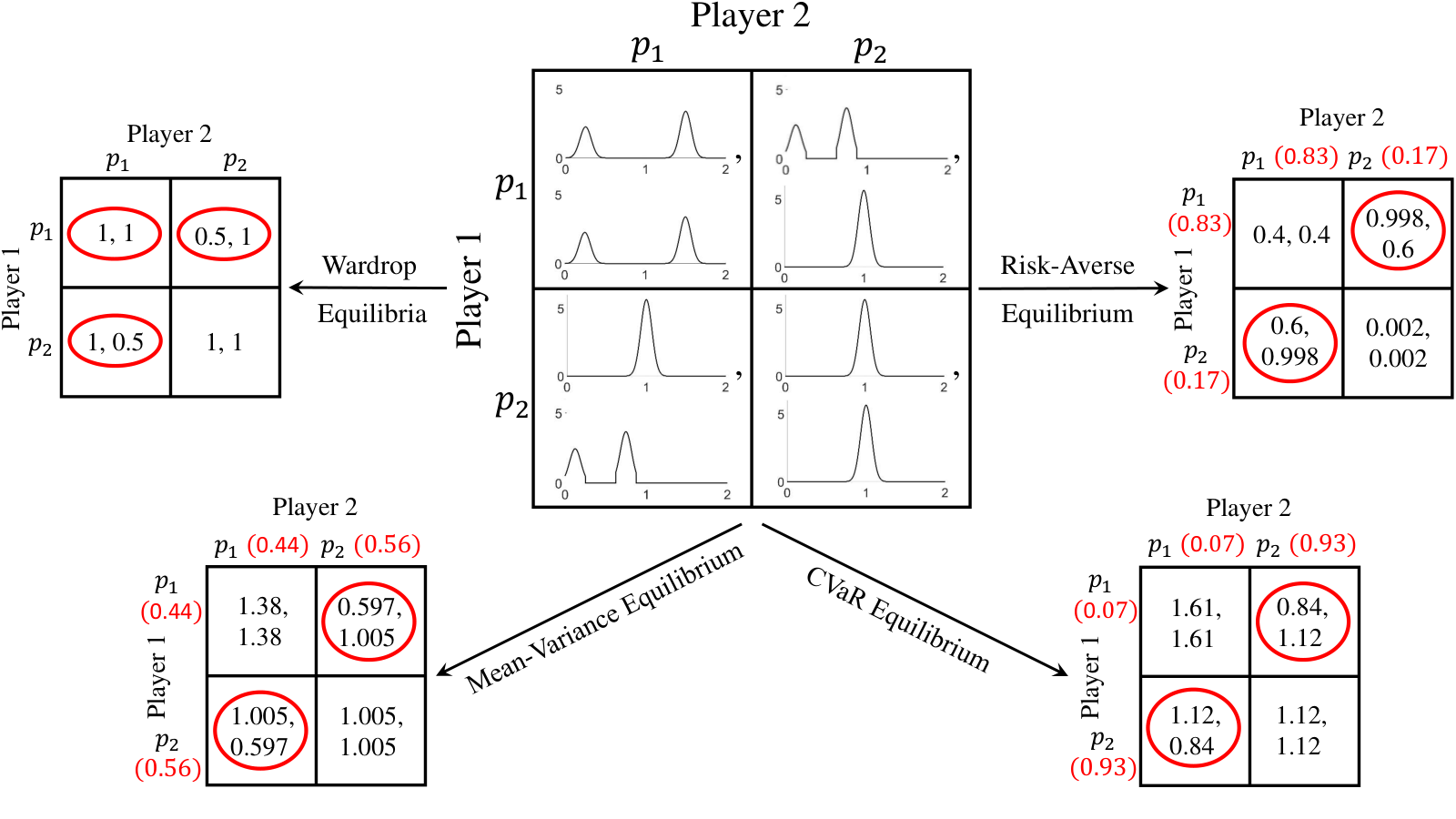
In the following, we present extra examples with the purpose of shedding light on drawbacks of the different equilibria in different scenarios and motivating more work to be done on a unified risk-averse framework. Furthermore, the following examples suggest that careful consideration should be given to the choice of the equilibrium that best fits the application of the interest.
5.1 Notes for Practitioners
The intention of this subsection is to direct the attention of practitioners planning to implement risk-averse in-vehicle navigation to cases in which each of the proposed risk-averse equilibria may provide travelers with counterintuitive guidance. To this end, three examples are discussed in the following to shed light on the implications of the three classes of risk-averse equilibria. The examples are meant to be simple to convey the idea in a straightforward manner.
Example 5.1
Consider a Pigou network with two parallel links, and , between source and destination. The travel times on links and are respectively independent random variables and with pdfs
where and are constants for which each of the two distributions integrate to one.
In Example 5.1, the means and variances of travel times along links and are , , , , respectively, and . As a result, although link has a higher variance than link , not only is link shorter than link in expectation, but link is shorter than link almost certainly. Hence, a rational traveler intends to take link for commute although its variance is higher than the variance of link . However, the mean-variance framework intends to keep a balance between lower expected travel time and lower uncertainty in travel time assuming that higher variance is against the spirit of risk-averse travelers. In Example 5.1, the mean-variance framework guides travelers to travel along link if , which is not optimal from the perspective of a risk-averse traveler. Note that both risk-averse equilibrium and CVaRα equilibrium for any guide travelers to traverse along link in this example.
Example 5.2
Consider a Pigou network with two parallel links, and , between source and destination. The travel times on links and are respectively independent random variables and with pdfs
where and are constants for which each of the two distributions integrate to one.
In Example 5.2, the means and variances of travel times along links and are , , , , respectively, and . Note that both distributions are the same over the interval ; however, the traveler has a better opportunity of experiencing shorter travel time on the lower quantile of the distribution of link compared to that of link . Hence, a rational traveler intends to take link for commute although its variance is higher than the variance of link . Furthermore, for ; hence, the CVaRα framework is indifferent between the two links when , which can result in a counterintuitive route selection in Example 5.2. The mean-variance framework also guides travelers to traverse along link if , which is not optimal from the perspective of a risk-averse traveler. Note that the risk-averse equilibrium guides travelers to traverse along link in this example as .
Example 5.3
Consider a Pigou network with two parallel links, and , between source and destination. The travel times on links and are respectively independent random variables and with pdfs
where and are constants for which each of the two distributions integrate to one.
In Example 5.3, the means and variances of travel times along links and are , , , , respectively, and . Although the expected travel time along link is less than that along link and it is more likely that the travel time along link is shorter than travel time along link , the travel time along link is concentrated around with probability which is somewhat larger than the concentration of travel time around when traveling along link . Hence, a risk-averse traveler may prefer to take link for commute although its expected travel time is higher than the expected travel time of link to avoid a long travel time. However, the risk-averse equilibrium guides travelers to traverse along link , which may not be optimal from the perspective of a risk-averse traveler. Note that the CVaRα equilibrium for and mean-variance equilibrium for guide travelers to traverse along link in this example.
6 Conclusion and Future Work
A stochastic atomic congestion game with incomplete information on travel times along arcs of a traffic/telecommunication network is studied in this work from a risk-averse perspective. Risk-averse travelers intend to make decisions based on probability statements regarding their travel options rather than simply taking the average travel time into account. In order to put this into perspective, we propose three classes of equilibria, i.e., risk-averse equilibrium (RAE), mean-variance equilibrium (MVE), and CVaRα equilibrium (CVaRαE). The MV and CVaRα equilibria are studied in the literature for networks with simplifying assumptions such as that the probability distributions of link delays are load independent or link delays are independent, which are not the case in this article. The notions of best responses in risk-averse, mean-variance, and CVaRα equilibria are based on maximizing the probability of traveling along the shortest path, minimizing a linear combination of mean and variance of path delay, and minimizing the expected delay at a specified risky quantile of the delay distributions, respectively. We prove that the risk-averse, mean-variance, and CVaRα equilibria exist for any finite stochastic atomic congestion game. Although proving bounds on the price of anarchy (PoA) is not the focus of this work, we numerically study the impact of risk-averse equilibria on PoA and observe that the Braess paradox may not occur to the extent presented originally and the PoA may improve upon using any of the proposed equilibria in both Braess and Pigou networks. Promising future directions are to study non-atomic, instead of atomic, stochastic congestion games in the proposed three classes of equilibria in their general case where the arc delay distributions are load dependent and not necessarily independent of each other, to find bounds on the price of anarchy for the proposed three classes of equilibria, and to find a unified class of equilibrium that captures risk-aversion for a broader class of travel time distributions in traffic/telecommunication networks.
References
- Aashtiani and Magnanti (1981) Aashtiani HZ, Magnanti TL, 1981 Equilibria on a congested transportation network. SIAM Journal on Algebraic Discrete Methods 2(3):213–226.
- Abdel-Aty, Kitamura, and Jovanis (1995) Abdel-Aty M, Kitamura R, Jovanis PP, 1995 Investigating effect of travel time variability on route choice using repeated-measurement stated preference data. Number 1493.
- Aghassi and Bertsimas (2006) Aghassi M, Bertsimas D, 2006 Robust game theory. Mathematical Programming 107(1-2):231–273.
- Altman et al. (2006) Altman E, Boulogne T, El-Azouzi R, Jiménez T, Wynter L, 2006 A survey on networking games in telecommunications. Computers & Operations Research 33(2):286–311.
- Angelidakis, Fotakis, and Lianeas (2013) Angelidakis H, Fotakis D, Lianeas T, 2013 Stochastic congestion games with risk-averse players. International Symposium on Algorithmic Game Theory, 86–97 (Springer).
- Bell (2009) Bell MG, 2009 Hyperstar: A multi-path astar algorithm for risk averse vehicle navigation. Transportation Research Part B: Methodological 43(1):97–107.
- Bell and Cassir (2002) Bell MG, Cassir C, 2002 Risk-averse user equilibrium traffic assignment: an application of game theory. Transportation Research Part B: Methodological 36(8):671–681.
- Braess (1968) Braess D, 1968 Über ein paradoxon aus der verkehrsplanung. Unternehmensforschung 12(1):258–268.
- Chabini (1997) Chabini I, 1997 A new algorithm for shortest paths in discrete dynamic networks. IFAC Proceedings Volumes 30(8):537–542.
- Chen and Ji (2005) Chen A, Ji Z, 2005 Path finding under uncertainty. Journal of advanced transportation 39(1):19–37.
- Chen and Zhou (2010) Chen A, Zhou Z, 2010 The -reliable mean-excess traffic equilibrium model with stochastic travel times. Transportation Research Part B: Methodological 44(4):493–513.
- Chen, Bell, and Bogenberger (2010) Chen Y, Bell MG, Bogenberger K, 2010 Risk-averse autonomous route guidance by a constrained a* search. Journal of Intelligent Transportation Systems 14(3):188–196.
- Connors and Sumalee (2009) Connors RD, Sumalee A, 2009 A network equilibrium model with travellers’ perception of stochastic travel times. Transportation Research Part B: Methodological 43(6):614–624.
- Correa, Hoeksma, and Schröder (2019) Correa J, Hoeksma R, Schröder M, 2019 Network congestion games are robust to variable demand. Transportation Research Part B: Methodological 119:69–78.
- Dial (1969) Dial RB, 1969 Algorithm 360: Shortest-path forest with topological ordering [h]. Communications of the ACM 12(11):632–633.
- Dijkstra (1959) Dijkstra E, 1959 A note on two problems in connection with graphs, numerical mathematics, vol. 1, pp. 269-271 .
- Dreyfus (1969) Dreyfus SE, 1969 An appraisal of some shortest-path algorithms. Operations research 17(3):395–412.
- Fan (2003) Fan Y, 2003 Optimal routing through stochastic networks. Ph.D. thesis, University of Southern California.
- Fonzone et al. (2012) Fonzone A, Schmöcker JD, Ma J, Fukuda D, 2012 Link-based route choice considering risk aversion, disappointment, and regret. Transportation research record 2322(1):119–128.
- Frank (1969) Frank H, 1969 Shortest paths in probabilistic graphs. Operations Research 17(4):583–599.
- Fu and Rilett (1998) Fu L, Rilett LR, 1998 Expected shortest paths in dynamic and stochastic traffic networks. Transportation Research Part B: Methodological 32(7):499–516.
- Fu, Sun, and Rilett (2006) Fu L, Sun D, Rilett LR, 2006 Heuristic shortest path algorithms for transportation applications: state of the art. Computers & Operations Research 33(11):3324–3343.
- Hall (1993) Hall E, 1993 Time-dependent, shortest-path algorithm for real-time intelligent vehicle highway system applications .
- Hall (1986) Hall RW, 1986 The fastest path through a network with random time-dependent travel times. Transportation science 20(3):182–188.
- Harsanyi (1967) Harsanyi JC, 1967 Games with incomplete information played by “Bayesian” players, i–iii part i. the basic model. Management science 14(3):159–182.
- Harsanyi (1968) Harsanyi JC, 1968 Games with incomplete information played by “Bayesian” players part ii. Bayesian equilibrium points. Management Science 14(5):320–334.
- Hayashi, Yamashita, and Fukushima (2005) Hayashi S, Yamashita N, Fukushima M, 2005 Robust nash equilibria and second-order cone complementarity problems. Journal of Nonlinear and Convex Analysis 6(2):283.
- Hosseini et al. (2017) Hosseini M, Jiang Y, Yekkehkhany A, Berlin RR, Sha L, 2017 A mobile geo-communication dataset for physiology-aware dash in rural ambulance transport. Proceedings of the 8th ACM on Multimedia Systems Conference, 158–163.
- Howard (2012) Howard RA, 2012 Dynamic probabilistic systems: Markov models, volume 1 (Courier Corporation).
- Kaufman and Smith (1993) Kaufman DE, Smith RL, 1993 Fastest paths in time-dependent networks for intelligent vehicle-highway systems application. Journal of Intelligent Transportation Systems 1(1):1–11.
- Kazimi, Brownstone, and Gosh (2000) Kazimi C, Brownstone A, Gosh T, 2000 Willingness-to-pay to reduce commute time and its variance: Evidence from the San Diego i-15 congestion pricing project. Transportation Research Board 79th Annual Meeting [CD-ROM], Washington, DC.
- Lam and Small (2001) Lam TC, Small KA, 2001 The value of time and reliability: measurement from a value pricing experiment. Transportation Research Part E: Logistics and Transportation Review 37(2-3):231–251.
- Lawler (1976) Lawler E, 1976 Combinatorial optimization: Networks and matroids. New York: Rinehart & Winston .
- Lo, Luo, and Siu (2006) Lo HK, Luo X, Siu BW, 2006 Degradable transport network: travel time budget of travelers with heterogeneous risk aversion. Transportation Research Part B: Methodological 40(9):792–806.
- Loui (1983) Loui RP, 1983 Optimal paths in graphs with stochastic or multidimensional weights. Communications of the ACM 26(9):670–676.
- Miller-Hooks and Mahmassani (2000) Miller-Hooks ED, Mahmassani HS, 2000 Least expected time paths in stochastic, time-varying transportation networks. Transportation Science 34(2):198–215.
- Mirchandani et al. (1986) Mirchandani B, Soroush H, Angrealtta G, Mason F, Serafini P, 1986 Routes and flows in stochastic networks. Advanced Schools on Stochastic in Combinatorial Optimization, eds G. Angrealtta, F. Mason and P. Serafini 129–177.
- Mirchandani and Soroush (1987) Mirchandani P, Soroush H, 1987 Generalized traffic equilibrium with probabilistic travel times and perceptions. Transportation Science 21(3):133–152.
- Mirchandani (1976) Mirchandani PB, 1976 Shortest distance and reliability of probabilistic networks. Computers & Operations Research 3(4):347–355.
- Murchland (1970) Murchland JD, 1970 Braess’s paradox of traffic flow. Transportation Research 4:391–394.
- Murthy and Sarkar (1996) Murthy I, Sarkar S, 1996 A relaxation-based pruning technique for a class of stochastic shortest path problems. Transportation science 30(3):220–236.
- Nash et al. (1950) Nash JF, et al., 1950 Equilibrium points in n-person games. Proceedings of the national academy of sciences 36(1):48–49.
- Neumann (1928) Neumann Jv, 1928 Zur theorie der gesellschaftsspiele. Mathematische annalen 100(1):295–320.
- Nie and Fan (2006) Nie Y, Fan Y, 2006 Arriving-on-time problem: discrete algorithm that ensures convergence. Transportation Research Record 1964(1):193–200.
- Nie (2011) Nie YM, 2011 Multi-class percentile user equilibrium with flow-dependent stochasticity. Transportation Research Part B: Methodological 45(10):1641–1659.
- Nie and Wu (2009) Nie YM, Wu X, 2009 Shortest path problem considering on-time arrival probability. Transportation Research Part B: Methodological 43(6):597–613.
- Nikolova and Stier-Moses (2011) Nikolova E, Stier-Moses NE, 2011 Stochastic selfish routing. International Symposium on Algorithmic Game Theory, 314–325 (Springer).
- Nikolova and Stier-Moses (2015) Nikolova E, Stier-Moses NE, 2015 The burden of risk aversion in mean-risk selfish routing. Proceedings of the Sixteenth ACM Conference on Economics and Computation, 489–506.
- Orda and Rom (1990) Orda A, Rom R, 1990 Shortest-path and minimum-delay algorithms in networks with time-dependent edge-length. Journal of the ACM (JACM) 37(3):607–625.
- Ordóñez and Stier-Moses (2010) Ordóñez F, Stier-Moses NE, 2010 Wardrop equilibria with risk-averse users. Transportation Science 44(1):63–86.
- Pierce (1975) Pierce A, 1975 Bibliography on algorithms for shortest path, shortest spanning tree, and related circuit routing problems (1956–1974). Networks 5(2):129–149.
- Pigou (1920) Pigou AC, 1920 The Economics of Welfare: By AC Pigou (Macmillan and Company, Limited).
- Pigou (2013) Pigou AC, 2013 The economics of welfare (Palgrave Macmillan).
- Schmöcker et al. (2009) Schmöcker JD, Bell MG, Kurauchi F, Shimamoto H, 2009 A game theoretic approach to the determination of hyperpaths in transportation networks. Transportation and traffic theory 2009: golden jubilee, 1–18 (Springer).
- Schrijver (2012) Schrijver A, 2012 On the history of the shortest path problem. Documenta Mathematica 17:155.
- Sigal, Pritsker, and Solberg (1980) Sigal CE, Pritsker AAB, Solberg JJ, 1980 The stochastic shortest route problem. Operations Research 28(5):1122–1129.
- Small (1999) Small KA, 1999 Valuation of travel-time savings and predictability in congested conditions for highway user-cost estimation, volume 431 (Transportation Research Board).
- Szeto, O’Brien, and O’Mahony (2006) Szeto W, O’Brien L, O’Mahony M, 2006 Risk-averse traffic assignment with elastic demands: Ncp formulation and solution method for assessing performance reliability. Networks and Spatial Economics 6(3-4):313–332.
- Tarjan (1983) Tarjan RE, 1983 Data structures and network algorithms, volume 44 (Siam).
- von Neumann and Morgenstern (1947) von Neumann J, Morgenstern O, 1947 Theory of games and economic behavior (Princeton University Press).
- Von Neumann and Morgenstern (1947) Von Neumann J, Morgenstern O, 1947 Theory of games and economic behavior, 2nd rev .
- Waller and Ziliaskopoulos (2002) Waller ST, Ziliaskopoulos AK, 2002 On the online shortest path problem with limited arc cost dependencies. Networks: An International Journal 40(4):216–227.
- Wardrop (1952) Wardrop JG, 1952 Road paper. some theoretical aspects of road traffic research. Proceedings of the institution of civil engineers 1(3):325–362.
- Wardrop and Whitehead (1952) Wardrop JG, Whitehead JI, 1952 Correspondence. some theoretical aspects of road traffic research. Proceedings of the Institution of Civil Engineers 1(5):767–768.
- Watling (2006) Watling D, 2006 User equilibrium traffic network assignment with stochastic travel times and late arrival penalty. European journal of operational research 175(3):1539–1556.
- Xiao and Lo (2013) Xiao L, Lo HK, 2013 Adaptive vehicle routing for risk-averse travelers. Procedia-Social and Behavioral Sciences 80:633–657.
- Xing and Zhou (2011) Xing T, Zhou X, 2011 Finding the most reliable path with and without link travel time correlation: A lagrangian substitution based approach. Transportation Research Part B: Methodological 45(10):1660–1679.
- Yekkehkhany et al. (2019) Yekkehkhany A, Arian E, Hajiesmaili M, Nagi R, 2019 Risk-averse explore-then-commit algorithms for finite-time bandits. 2019 IEEE 58th Conference on Decision and Control (CDC), 8441–8446.
- Yekkehkhany et al. (2020) Yekkehkhany A, Arian E, Nagi R, Shomorony I, 2020 A cost-based analysis for risk-averse explore-then commit finite-time bandits .
- Yekkehkhany, Murray, and Nagi (2020) Yekkehkhany A, Murray T, Nagi R, 2020 Risk-averse equilibrium for games. arXiv preprint arXiv:2002.08414 .
- Zeng et al. (2015) Zeng W, Miwa T, Wakita Y, Morikawa T, 2015 Application of lagrangian relaxation approach to -reliable path finding in stochastic networks with correlated link travel times. Transportation Research Part C: Emerging Technologies 56:309–334.
Appendix A Proof of Theorem 4.5
Let be the risk-averse best response function where . It is easy to see that the existence of a fixed point for the risk-averse best response function, i.e., , proves the existence of a risk-averse equilibrium. The following four conditions of the Kakutani’s Fixed Point Theorem are shown to be satisfied for the function to prove the existence of a fixed point for the function.
- 1.
The domain of function is a non-empty, compact, and convex subset of a finite dimensional Euclidean space: is the Cartesian product of non-empty simplices as each player has at least one strategy to play; furthermore, each of the elements of is between zero and one, so is non-empty, convex, bounded, and closed containing all its limit points.
- 2.
, : The set in Equation (3) is non-empty as maximum exists over a finite number of values. As a result, is non-empty for all since it is the set of all probability distributions over the corresponding mentioned non-empty set.
- 3.
The co-domain of function is a convex set for all : It suffices to prove that is a convex set for all and for all . For any , if , we need to prove that for any and for any . Let the supports of and be defined as and , respectively. It is concluded from the definition of the risk-averse best response in Definition 4.3 that , which results in . As a result, using the definition of risk-averse best response, any probability distribution over the set is a risk-averse best response to . It is trivial that the mixed strategy is a valid probability distribution over the set for any , so for any and for any that completes the convexity proof of the set .
- 4.
has a closed graph: has a closed graph if for any sequence with for all , we have . Proof by contradiction is used to show that has a closed graph. Consider by contradiction that does not have a closed graph, so there exists a sequence with for all , but . As a result, there exists some such that . Using the definition of risk-averse best response in Definition 4.3, there exists , , and some such that
(31) Since the latencies over edges are continuous random variables and , for any , there exists a sufficiently large such that we have the following for :
(32) By adding inequalities with the same direction in Equations (31) and (32), for we have
(33) For the same reason as of Equation (32), for any , there exists a sufficiently large such that we have the following for :
(34) where . By adding the inequalities with the same direction in Equations (33) and (34), for we have
(35) Equation (35) contradicts the fact that , which completes the proof that has a closed graph.
As listed above, the risk-averse best response function satisfies the four conditions of Kakutani’s Fixed Point Theorem. As a direct result, for any finite -player stochastic congestion game, there exists such that , which completes the existence proof of a risk-averse equilibrium for such games.
Appendix B Proof of Theorem 4.9
Let be the mean-variance best response function where . It is easy to see that the existence of a fixed point for the mean-variance best response function, i.e., , proves the existence of a mean-variance equilibrium. The following four conditions of the Kakutani’s Fixed Point Theorem are shown to be satisfied for the function to prove the existence of a fixed point for the function.
- 1.
The domain of function is a non-empty, compact, and convex subset of a finite dimensional Euclidean space: is the Cartesian product of non-empty simplices as each player has at least one strategy to play; furthermore, each of the elements of is between zero and one, so is non-empty, convex, bounded, and closed containing all its limit points.
- 2.
, : The set in Equation (9) is non-empty as minimum exists over a finite number of values. As a result, is non-empty for all since it is the set of all probability distributions over the corresponding mentioned non-empty set.
- 3.
The co-domain of function is a convex set for all : It suffices to prove that is a convex set for all and for all . For any , if , we need to prove that for any and for any . Let the supports of and be defined as and , respectively. It is concluded from the definition of the mean-variance best response in Definition 4.7 that , which results in . As a result, using the definition of mean-variance best response, any probability distribution over the set is a mean-variance best response to . The mixed strategy is obviously a valid probability distribution over the set for any , so for any and for any that completes the convexity proof of the set .
- 4.
has a closed graph: has a closed graph if for any sequence with for all , we have . Proof by contradiction is used to show that has a closed graph. Consider by contradiction that does not have a closed graph, so there exists a sequence with for all , but . As a result, there exists some such that . Using the definition of mean-variance best response in Definition 4.7, there exists , , and some such that
(36) Since the latencies over edges are continuous random variables and , for any , there exists a sufficiently large such that we have the following for :
(37) By adding inequalities with the same direction in Equations (36) and (37), for we have
(38) For the same reason as of Equation (37), for any , there exists a sufficiently large such that we have the following for :
(39) where . By adding the inequalities with the same direction in Equations (38) and (39), for we have
(40) Equation (40) contradicts the fact that , which completes the proof that has a closed graph.
As listed above, the mean-variance best response function satisfies the four conditions of Kakutani’s Fixed Point Theorem. As a direct result, for any finite -player stochastic congestion game, there exists such that , which completes the existence proof of a mean-variance equilibrium for such games.
Appendix C Proof of Theorem 4.13
Let be the CVaRα best response function where . It is easy to see that the existence of a fixed point for the CVaRα best response function, i.e., , proves the existence of a CVaRα equilibrium. The following four conditions of the Kakutani’s Fixed Point Theorem are shown to be satisfied for the function to prove the existence of a fixed point for the function.
- 1.
The domain of function is a non-empty, compact, and convex subset of a finite dimensional Euclidean space: is the Cartesian product of non-empty simplices as each player has at least one strategy to play; furthermore, each of the elements of is between zero and one, so is non-empty, convex, bounded, and closed containing all its limit points.
- 2.
, : The set in Equation (19) is non-empty as minimum exists over a finite number of values. As a result, is non-empty for all since it is the set of all probability distributions over the corresponding mentioned non-empty set.
- 3.
The co-domain of function is a convex set for all : It suffices to prove that is a convex set for all and for all . For any , if , we need to prove that for any and for any . Let the supports of and be defined as and , respectively. It is concluded from the definition of the CVaRα best response in Definition 4.11 that , which results in . As a result, using the definition of CVaRα best response, any probability distribution over the set is a CVaRα best response to . The mixed strategy is obviously a valid probability distribution over the set for any , so for any and for any that completes the convexity proof of the set .
- 4.
has a closed graph: has a closed graph if for any sequence with for all , we have . Proof by contradiction is used to show that has a closed graph. Consider by contradiction that does not have a closed graph, so there exists a sequence with for all , but . As a result, there exists some such that . Using the definition of CVaRα best response in Definition 4.11, there exists , , and some such that
(41) Since the latencies over edges are continuous random variables and , for any , there exists a sufficiently large such that we have the following for :
(42) By adding inequalities with the same direction in Equations (41) and (42), for we have
(43) For the same reason as of Equation (42), for any , there exists a sufficiently large such that we have the following for :
(44) where . By adding the inequalities with the same direction in Equations (43) and (44), for we have
(45) Equation (45) contradicts the fact that , which completes the proof that has a closed graph.
As listed above, the CVaRα best response function satisfies the four conditions of Kakutani’s Fixed Point Theorem. As a direct result, for any finite -player stochastic congestion game, there exists such that , which completes the existence proof of a CVaRα equilibrium for such games.