Full Quaternion Representation of Color images: A Case Study on QSVD-based Color Image Compression

Alireza Parchami Mojtaba Mahdavi Affiliation: [1ex] Department of Computer Engineering Affiliation: University of Isfahan, Iran Affiliation: alirezaprm@mehr.ui.ac.ir, m.mahdavi@eng.ui.ac.ir

1. Introduction

Image Processing and Computer Vision are widely used in many different applications and have a dominant role in industries and our lives. The increasing number of applications using color images makes image processing a crucial point in artificial intelligence. Therefore, we have witnessed rapid enhancement in different algorithms and applications derived from image processing and computer vision in many fields.

Throughout history, colors in images have seen dramatic changes. During the 20th century, black-and-white images were mostly used. Since a black-and-white image only represents intensity levels, it forms a 2D matrix consists of real numbers. As a result, the processing procedure is not complicated due to the existence of one 2D matrix. By color images, which each of them consists of three separate 2D matrices, the processing procedure would be controversial. Since there has been no holistic approach for color image processing that considers the image as one entity, two approaches are mostly used for color images that none of them is efficient enough. The first approach tries to convert a color image into a grayscale one and only cares about the intensity levels, which means it completely neglects the colors. The second approach, however, separates a color image into three scalar matrices to be processed individually by different algorithms and be masked by various filters. However, this approach is neither comprehensive nor efficient due to ignoring cross-correlation by channel separation.

The idea of using quaternion numbers in color image processing was introduced in 1996 by Sangwine, using the discrete version of Ell's Quaternion Fourier Transforms [1]. By this technique, image processing in a holistic way was made possible since quaternions empower us to consider an image as one matrix in a holistic space. This approach also enabled us to consider cross-correlation while processing color images. However, there were two main disadvantages that prevented this approach to be as much time- and space-efficient as it could be. Therefore, two other alternatives were introduced to alleviate the issues, but they also had some problems, which are completely discussed in Section 2: Related Works.

The research reported in this paper aims to introduce a method for image processing in a holistic way using full quaternion numbers, which treats the color image as a vector field that has four highly correlated dimensions, in order to exploit the maximum potential of auto- and cross-correlation of color channels.

In addition to introducing a model for full quaternion representation of color images, a compression method based on the proposed representation and Quaternion Singular Value Decomposition (QSVD) was presented in this paper as a case study. This method was evaluated by UCID dataset, and was compared with another compression method that uses pure quaternion numbers.

2. Related Works

It is believed that there are correlations between adjacent pixels of an image, whether color or grayscale one, and we can consider local correlations in different parts of an image. Chrominance and luminance change so slightly in adjacent pixels, and there is no dramatic difference between them. That is, each subpixel in R, G and B channels at coordination $(i,j)$ is correlated with its corresponding adjacent subpixels. This concept is also referred to as auto-correlation, which indicates the similarity of a signal with itself, and it was defined for pure quaternion representation of color images [2]. Figure 1 shows adjacent pixels of the green channel in a local area that are highly similar, and the difference from one subpixel to its neighbours is subtle.

Refer to caption — Figure 1: Auto-correlation of adjacent pixels in green channel

For color images, in addition to auto-correlation, there are correlations between the color channels. Capturing the inherent correlations between color channels and taking them into account, can indeed demonstrate more information than the conventional approach, which color channels were processed separately and the individual output results were combined. The concept of correlation between channels is referred to as cross-correlation, which indicates the similarity of two distinct signals, and it was defined and proved applicable for quaternion representation of color images [2, 3]. Using cross-correlation is one of the main motivations to adopt quaternions for digital color image processing.

Many methods have tried to introduce new ways of processing to enhance the efficiency of image processing and computer vision concerning the correlation of color channels. When it came to color image processing, we mainly relied on grayscale images due to the higher inherent complexity of color images and the difficulty of considering the 3D space of color images as one entity. Therefore, two basic approaches were taken toward image processing and computer vision. In the first approach, a color image was transformed into a grayscale image by using either Rec. BT.601 [4]

Gray=(0.299Red+0.587Green+0.114Blue)

or Rec. BT. 709 recommended by ITU-R¹¹ 1 International Telecommunication Union Radiocommunication Sector [5]:

Gray=(0.2126Red+0.7152Green+0.0722Blue)

By this conversion, the images was considered as a 2D grayscale matrix, and then the matrix was processed by desirable algorithms. In this case, none of the objects was distinguishable with their colors. Although this approach would be fast enough and easy to compute, it was not appropriate for many applications because the colors of objects can indeed indicate significant features, and the cross-correlation between three channels can offer useful information.

The idea of using color channels for color image processing sparked by using separate channels for primary colors, which are red, green and blue. This approach, which tried to consider colors of objects, separated a color image into three distinct channels. Therefore, we had three 2D matrices as a consequence of having three channels for color images and treated each of them as a grayscale image. Whether we used neural networks or other image processing techniques, the cross-correlation between channels was not taken into consideration due to the channel separation in this approach. As a result, we lost data related to the cross-correlation of the color channels at the very beginning step of the process because we did not consider a color image as one unique entity.

In 1998, Sangwine proposed a method based on quaternion numbers that applied the benefits of quaternion numbers into color image processing. In this method, a color image was considered as one matrix consists of pure quaternion numbers, and the matrix was processed in a holistic space. To convert an RGB image to quaternion matrix, RGB channels were simply put into the vector part of the quaternion matrix. Thus, a quaternion matrix $f_{q}(m,n)$ , which represents a color image, was formed as[1, 6]

f_{q}(m,n)=f_{R}(m,n)i+f_{G}(m,n)j+f_{B}(m,n)k

where $f_{R}(m,n)$ , $f_{G}(m,n)$ and $f_{B}(m,n)$ correspond to red, green and blue channels of the color image. By this representation, the scalar part of the matrix was actually considered as zero, which means a channel with no information. Thus, the final representation is like:

$f_{q}(m,n)=0+f_{R}(m,n)i+f_{G}(m,n)j+f_{B}(m,n)k$

In the rest of this paper, we call this approach as pure quaternion representation because it only deals with vector part of the quaternion matrix. As a consequence of the development of quaternion mathematical operations, many applications such as splicing detection [7], watermarking [8, 9, 10, 11, 12, 13], filter implementation [14, 15, 16], image classification [17], image sparse representation [18] and quaternion-type moment [19] have treated color images holistically as a vector field using the pure quaternion representation for the last 20 years.

This representation empowers us to use various quaternion mathematical operations for processing the image matrix comprehensively concerning the auto- and cross-correlation. However, it does not benefit from all components of a quaternion matrix and only concerns about the vector part, which leads to the fact that the maximum potential of quaternions is not being used. To illustrate more, with image processing using pure quaternion numbers, we have to deal with a new channel filled with zeros for the real component of the quaternion matrix. This way, a three-channel color image is actually considered as part of a four-channel image with an extra black channel that has no correlation with others and is completely unrelated with each of the channels conveying specific information. It can make procedures of processing more complicated since quaternion mathematical operations, such as QDCT or QSVD, consider all components of the quaternions and have to take a new channel into consideration which is irrelevant to others. Furthermore, the method increases both the size of the matrix and time of processes due to adding a new channel with the same size of the other channels [20], which leads to having four 2-D matrices with the same number of columns and rows as the original image.

As an alternative, a new type of representation was introduced based on trinion numbers, which have one real and two imaginary units. In this approach, a color image was represented as [20]:

$f_{q}(m,n)=f_{R}(m,n)+f_{G}(m,n)i+f_{B}(m,n)j$

This representation aimed to avoid adding a new channel and assign one component to each of the RGB channels. Some mathematical operations were also generalized to trinions for this purpose. However, only few color image processing works adopted trinion representation because the theory of trinions has not enough developed compared with the theory of quaternions [20].

As another alternative, some scientists developed another method that tries to use all four components of quaternion numbers. In this method, they captured more information and measured the depth of color images and used quaternion numbers to combine both color and depth information for different purposes such as RGB-D object recognition [21] or color image splicing detection [22]. Therefore, the quaternion matrix was formed as:

\begin{split}f_{q}(m,n)&=f_{D}(m,n)+f_{R}(m,n)i\\ &+f_{G}(m,n)j+f_{B}(m,n)k\end{split}

where $f_{D}(m,n)$ indicates the depth information. Although it has been proved to be a good technique for adopting all components of quaternion numbers, it needs additional devices to measure the depth information while capturing the photos such as Kinect, and it is not possible to use this method with ordinary cameras [21, 22]. This is the main reason that the full quaternion representation with RGB-D information has not been used widely for image processing.

With regard to the application of QSVD, color image compression is one of the fields that quaternions can be used, and singular value decomposition (SVD) is a classical mathematical tool that has been used for a long time to compress grayscale and color images. Quaternion singular value decomposition (QSVD) is the quaternion version of this useful tool and has exploited in color image processing [1, 23]. Therefore, color image compression using QSVD became possible, and it has been proved to be an appropriate application. Both SVD-based image compression using three separated channels and QSVD-based image compression using pure quaternion representation were implemented and compared with each other by Ying Li [24]. Although the comparison was entirely on the favour of SVD-based color image compression, the main downsides of QSVD-based color image compression were proved to be the long time required for QSVD calculation and lower compression rate (CR). In this paper, QSVD is used to compress color images using the full quaternion representation to put our method into practice. To solidify our compression method with full quaternion numbers, we implemented this compression method on both pure quaternion and full quaternion representations to compare them with each other.

3. Methodology

As mentioned in section 2, the pure quaternion representation processed color images comprehensively concerning the auto- and cross-correlation. However, the extra fourth dimension not only diluted the correlation of color channels but also increased processing time and matrix size. The trinion numbers tried to use correlation more effectively than the previous work, but its mathematical concepts have not been well-developed. Moreover, using RGB-D color space for quaternion representaiton required special devices that are not feasible in most of the times.

Regarding using all components of quaternion numbers, we sought for an approach which converts an RGB image into a full quaternion matrix to use quaternion mathematical operations and process images comprehensively. By this method, not only do we take full advantage of quaternion mathematical concepts and treat with color image as a full quaternion matrix, but also we use four correlated 2D matrices with a reduction in the number of columns to form the quaternion matrix that culminates in a cutback in the size and time of processing. Besides, no additional devices is needed in this approach to transform a color image into a full quaternion matrix. In the rest of this paper, we call this approach as full quaternion representation.

In the rest of this section, at first, a broad overview of the key mathematical concepts and tools used in this research are provided. Afterwards, we propose a method using an autoencoder to generate a global model and then, use the model to transform an RGB image into a quaternion one. subsequently, quaternion image compression is introduced as a case study of the proposed method.

3.1. Background

3.1.1. Quaternion Numbers

Quaternion numbers, also known as hyper-complex numbers, consist of one scalar and one vector part that has three imaginary units. In fact, a quaternion $q$ is an element of the 4-D normed algebra with basis ${1,i,j,k}$ . Quaternion number $q$ is represented in the form

q=a+bi+cj+dk

where $a,b,c,d\in\mathbb{R}$ are called components and $i,j,k$ are fundamental quaternion units [25]. Rules of the product of fundamental units are defined by

$\displaystyle ij$	$\displaystyle=-ji=k$	(1)
$\displaystyle jk$	$\displaystyle=-kj=i$
$\displaystyle ki$	$\displaystyle=-ik=j$
$\displaystyle ijk$	$\displaystyle=i^{2}=j^{2}=k^{2}=-1$

A quaternion $q\in\mathbb{H}$ can²² 2 Classically denoted by $\mathbb{H}$ in honor of Sir W.R. Hamilton who discovered them in 1843 be decomposed into a scalar part $S(q)$ and a vector part $V(q)$ :

q=S(q)+V(q)

where

S(q)=a,\ V(q)=bi+cj+dk

The quaternion $q$ is called pure quaternion if $S(q)=0$ . It is normally known as a real number if $V(q)=0$ , and it is called full quaternion if none of the scalar and vector parts are zero³³ 3 $V(q)\neq 0$ if at least one of the components $b,c,d$ is non zero.. Note that the multiplication of two quaternion numbers $p,q\in\mathbb{H}$ is not commutative due to the relation between fundamental units in (1), but it is associative for three quaternion $p,q,r\in\mathbb{H}$ [26]:

p\times q\neq q\times p

(p\times q)\times r=p\times(q\times r)

Moreover, the conjugate of a quaternion, which is denoted by $\bar{q}$ or $q^{*}$ , is defined as

\bar{q}=a-bi-cj-dk

3.1.2. Autoencoder

A Feedforward autoencoder is a type of artificial neural networks. It has the same number of nodes in input and output, and it tries to encode data in the latent layer with the purpose of reconstructing the input based on the encoded data. The connections do not form a cycle, and the nodes of the middle layers would vary widely. It is an unsupervised learning process which pursues encoding inputs into a desirable number of nodes efficiently to recover them as accurately as possible. Figure 2 shows the elements of an autoencoder.

In an autoencoder, the existence of hidden layers is not compulsory. That is, the number of encoder and decoder hidden layers would vary widely according to researchers’ purpose. However, the latent space is the key layer since input data are encoded in this layer and then, the encoded data are used for processing.

3.1.3. Quaternion Singular Value Decomposition (QSVD)

Singular Value Decomposition (SVD) is a well-known linear algebra technique which represents a matrix $A$ in a coordinate system where the covariance matrix is diagonal. SVD has been proved as an image compression method, which generalizes the eigendecomposition of a matrix by the extension of polar decomposition. The SVD of a matrix $A\in\mathbb{R}^{m\times n}$ is given as:

A=U\Sigma V^{T}

where $U\in\mathbb{R}^{m\times m}$ is left singular vector, $\Sigma\in\mathbb{R}^{m\times n}$ stands for singular values, and $V\in\mathbb{R}^{n\times n}$ is right singular vector. This concept has also been extended to quaternion numbers, known as quaternion singular value decomposition (QSVD) [27]. The proof of Quaternion Polar Decomposition and Quaternion Singular Value Decomposition is given in [28] .

There is a QSVD for every quaternion matrix $Q\in\mathbb{H}^{N\times M}$ given as:

Q=U\Sigma V^{\triangleleft}

where ^⊲ stands for conjugate transposition, $U\in\mathbb{H}^{N\times N}$ indicates left singular vector and $V\in\mathbb{H}^{M\times M}$ indicates right singular vector. $U$ and $V$ are unitary quaternion matrices, which means

S(UU^{\triangleleft})=S(VV^{\triangleleft})=I

and

V(UU^{\triangleleft})=V(VV^{\triangleleft})=O

where $S(x)$ and $V(x)$ denote the scalar and vector parts of the quaternions, respectively. In the notation, $I$ is the identity matrix (diagonal matrix of ones) and $O$ is a matrix contains only zeros [28, 29]. The same as SVD, $\Sigma\in\mathbb{R}^{m\times n}$ indicates singular values of the quaternion matrix $Q$ .

Having a compressed image based on SVD, the number of preserved columns of $U,\Sigma$ and $V$ indicates the level of compression. That is, we can modify the quality of the compressed image and the size of the compressed file by matrix truncation, which means adopting the $t\in\mathbb{N}$ largest singular values and the corresponding vectors of the left and right unitary matrices, and leaving the rest of the values as zero [24]. As the real values of $\Sigma$ arranged in decreasing magnitude order along the diagonal, the first $t$ values carry the most significant decomposition values and have a vital role in image reassembling.

3.2. Proposed Method

Taking local correlation into account, we looked for a relationship that enables us to represent a color image with four 2D real matrices, which all of them are highly correlated, to create a full quaternion matrix. For this purpose, we considered a pair of adjacent pixels at coordinations $(i,j)$ and $(i,j+1)$ where $i$ and $j$ indicate the position of row and column of pixels, respectively. Because of colorfulness of the image, we have 3 sub-pixel values in RGB color space for each pixel. Thus, there are six values for the pair above:

	$\displaystyle R(i,j)$	$\displaystyle,G(i,j),B(i,j)$
	$\displaystyle R(i,j+1)$	$\displaystyle,G(i,j+1),B(i,j+1)$

We used a full connect feedforward autoencoder to find coefficients and biases for these six subpixels to generate a model that transforms each pair of pixels into four numbers that can form a full quaternion number. Using this model for all pairs of adjacent pixels in a color image, we formed a quaternion matrix with the same number of rows as the original image and the half number of columns because each pair of adjacent pixels in RGB color space at coordinations $(i,j)$ and $(i,j+1)$ is transformed into one quaternion number. Figure 3 shows the size of both original and quaternion matrices with differences in their second and third dimensions. Original matrix is considered as a 3-D matrix of integer numbers with the size of $N\times M$ , while the quaternion matrix is a 2-D matrix of quaternion numbers with the size of $N\times\frac{M}{2}$ .

It is notable that prior to transforming a color image into a full quaternion matrix, if the image has odd number of columns, replicate padding⁴⁴ 4 In replicate padding,values outside the boundary are set equal to the nearest image border value[32]. is used to make the number of columns even. This is because we have to consider pixels two by two in order to form the quaternion matrix.

Like every color space that each component carries particular features, each component of the quaternion matrix contains specific information from the original image. Figure 4 shows each component of the quaternion matrix that was acquired from the generated model. After processing the quaternion matrix and implementing algorithms with quaternion mathematical operations, the same model was used to revert the full quaternion matrix to RGB color space in order to use the image in normal applications. That is, we decoded the encoded data to reach the RGB pixels.

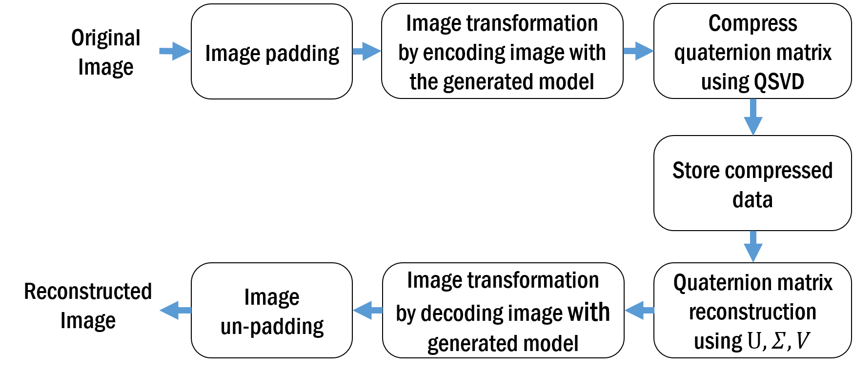
As a case study, image compression can be used as an appropriate practical application for representing an RGB image with a quaternion matrix [25, 30, 31]. Figure 5 shows the diagram of color image compression quaternion numbers.

Compression was done in three steps. As the calculation time of both of the SVD and QSVD would increase exponentially with higher resolution of images, block splitting was done to enhance the calculation time. Therefore, we tried to reach the most suitable block size concerning the QSVD calculation time and the quality of image. QSVD was calculated for each block and it was truncated by $t$ , which is our modifiable measure for compression. Finally, the truncated $U$ , $\Sigma$ and $V$ matrices were compressed by RAR algorithm using WinRAR software by setting compression method as best. Figure 6 illustrates on the steps of QSVD-based color image compression utilizing the generated model and the proposed full quaternion representation.

The quaternion matrix can be reconstructed by the formula of:

ReconstructedQuaternionMatrix=U\Sigma V^{\triangleleft}

Finally, the full quaternion matrix was decoded into a 3-D matrix of RGB by using the model generated by the designed autoencoder.

3.3. Methodology Parameters

We used a full connect feedforward autoencoder to find a global model for color image conversion into a full quaternion matrix. The autoencoder had 6 nodes for input and output layers as it received and predicted 6 subpixels of two adjacent color pixels as mentioned. It had 4 nodes in latent space and there was no hidden layer in the encoder and decoder. We also used pure linear activation function and L2 regularization method to train autoencoder with UCID dataset, so the model could be known as a regression model, which can also be considered as a lossy convertor. 60% of the available UCID dataset was used for training and the rest of it was used for testing⁵⁵ 5 The official website of UCID dataset has been out of access, and there is no other official alternative source for this dataset. The only available website is http://jasoncantarella.com/downloads. However, the dataset uploaded on this website is incomplete and contains only the first 886 images of the dataset. Therefore, we have succeeded to train the autoencoder with 536 randomly selected images (60% of the available dataset) and test the proposed method with the remaining 350 images of UCID dataset. [33].

4. Results

The quality of a reconstructed image is the primary key to evaluate the proposed model and compression method. We used 40% of the available UCID dataset for assessing the model and compression method since UCID dataset provides a wide range of raw images in many different categories. We also used three methods for measuring the performance of the model for color iamge transformation to a quaternion matrix, namely SSIM, PSNR and MSE. Moreover, to evaluate the quaternion color image compression, we used PSNR, Compression Ratio (CR) and MSE for each of the color channels. The methods for measurement are the following four.

$\bullet$ MSE: calculated for each channel separately and is given as:

MSE=\frac{1}{N*M}\sum_{i=0}^{N-1}\sum_{j=0}^{M-1}{[I_{1}(i,j)-I_{2}(i,j)]}^{2}

Where $N$ and $M$ are the number of rows and columns of matrix , and $I1$ and $I2$ are the input and output matrix.

$\bullet$ PSNR: which is given as:

PSNR=10\log_{10}{\frac{MAX_{I}^{2}}{MSE}}\\ =20\log_{10}{MAX_{I}}-10\log_{10}{MSE}

Where $MAX_{I}$ is the maximum possible value in matrix I, which is 255 for 24-bit color (true color) images.

$\bullet$ SSIM: which is given as:

SSIM=\frac{(2\mu_{I_{1}}\mu_{I_{2}}+C_{1})(2\sigma_{{I_{1}}{I_{2}}}+C_{2})}{(\mu_{I_{1}}^{2}+\mu_{I_{2}}^{2}+C_{1})(\sigma_{I_{1}}^{2}+\sigma_{I_{2}}^{2}+C_{2})}

Where $I_{1}$ and $I_{2}$ are original and reconstructed images; $\mu_{I_{1}}$ and $\mu_{I_{2}}$ are the average of $I_{1}$ and $I_{2}$ respectively; $\sigma_{I_{1}}^{2}$ and $\sigma_{I_{2}}^{2}$ are the variance of $I_{1}$ and $I_{2}$ respectively; $\sigma_{{I_{1}}{I_{2}}}$ is the covariance of $I_{1}$ and $I_{2}$ ; and

C1=(K_{1}L)^{2},\;\;C2=(K_{2}L)^{2}

with $K_{1}=0.01$ , $K_{2}=0.03$ and $L=255$ .

$\bullet$ Compression Ratio: which is straightforwardly given as:

CR=\frac{Uncompressed\ Size}{Compressed\ Size}

4.1. Transformation

Using a global model for encoding 2 adjacent pixels into one quaternion number based on local correlation leads to a lossy conversion. Although an adequate model and high correlated pixels can compensate for the reduction of the quality of reconstructed images, the act of encoding and decoding are lossy. Table 1 shows the results of PSNR, SSIM and MSE of the generated model performed on the UCID dataset. Images were straightly encoded and decoded without any additional filters or processes.

PSNR	SSIM	MSE
PSNR	SSIM	Red	Green	Blue
41.2496	0.9931	1.4578	0.7034	1.3184

Table 1: Assessment of the generated model on UCID dataset

The results in table 1 are good indicative of this fact that the act of encoding and decoding does not have distinguishable impact on images and can not be noticed by humans due to its low loss. The small values of MSE, especially in green channel, demonstrate that the differences between original and reconstructed pixels are pretty low, which can even be considered as a suitable method for image processing by machines and computers.

Since the model is actually a type of a regression model, edges of images needs closer attention. We considered Big Ben in figure 7 for model performance testing on photos full of edges. The sheer number of edges in this image makes it a perfect choice for this test. PSNR of 43.5667 and SSIM of 0.9990 show that the model encoded the photo into a full quaternion matrix and reconstructed the RGB image perfectly. The reason for this low amount of loss stands for the fact that the state of colors does not change dramatically in edge areas. That is, the chrominance and luminance change marginally in several arrays of pixels, and the auto-correlation and cross-correlation in the edges are still high. Therefore, the model performed well in these situations, and we can still count on the high correlation of corresponding subpixels in adjacent pixels.

4.2. Quaternion Image Compression

In this section, PSNR, MSE and Compression Ratio are presented for the proposed full quaternion compression method. The same measures for pure quaternion compression method are taken in section V: Discussion, where both methods are compared with each other.

In the proposed compression method, the calculation time for QSVD would be a discussing area. As QSVD considers all components of quaternion numbers comprehensively, the time of QSVD would last more than the calculation time of SVD on three separated 2D - matrices that contain only real numbers. Figure 8 shows the calculation time of QSVD of the proposed full quaternion representation splitted into $n\times n$ blocks, with $n=16,32,64,128,256$ . According to this figure, the most time-efficient block size for QSVD calculation is 64, which needs 3.8924 seconds on average using Intel® Core^TM i5-7400 processor, Matlab® R2017b, and Quaternion toolbox for Matlab[34].

Figure 9 depicts the results of measuring PSNR for compressed images. The size of compressed images were modified by adopting different $t$ for truncation of $U,\Sigma$ and $V$ . Greater $t$ equals more preserved data in the matrices $U,\Sigma$ and $V$ , which leads to higher quality and bigger file size. Based on this chart, block sizes of $32\times 32$ and $64\times 64$ have the best results because they have higher PSNR in the same compressed file size.

Compression ratio (CR) depends on $n$ , which indicates the size of blocks for block splitting, and $t$ , which indicates the number of preserved columns after matrix truncation. Figure 10 demonstrates the CR measure for various $t$ 's and $n$ 's.

Taking all measures above into account, the $64\times 64$ and $32\times 32$ block sizes seem to be the most efficient choices because they have faster QSVD calculation time and higher PSNR in the same file size. The compression method using $64\times 64$ blocks is faster while the method using $32\times 32$ blocks has a higher quality in the same compressed file size for PSNR lower than 38. As a result of better performance of these two block sizes, MSE for red, green and blue channels are given only for $32\times 32$ and $64\times 64$ block sizes in the figure 11.

Since the Cone cells are responsible for color perception in daylight (Photopic), human eyes are more sensitive to greenish-yellow light than any other color because it stimulates medium and long cone types. However, in weak light, Rod cells are more brilliant for color perception (Scoptopic), and they are more sensitive to blueish-green wavelength. These two facts, which are shown in figure 12, contribute to the notion that human eyes are more sensitive to green color than blue and red [35]. Based on the table 1 and figure 11, green, which is the most significant color for human eyes, has the least amount of error than the other colors in our proposed full quaternion representation and quaternion compression method, and this makes both of the proposed representation and compression very useful for common photography.

5. Discussion

In this section, the pure quaternion and full quaternion compression methods are compared with each other. The same as previous section, the QSVD calculation time, PSNR, compression ratio (CR) and MSE are evaluated.

According to figure 8, the QSVD calculation would take considerable time. However, since our full quaternion method reduces the number of columns of images by half, it needs much less time for QSVD calculation compared with pure quaternion approach. As mentioned in section II, the act of adding a new channel with the same size as original channels in pure quaternion representation increases the time of processing. The figure 13 indicates the comparison of QSVD calculation time for both of the discussed methods considering block sizes of 16, 32, 64, 128 and 256.

Since the QSVD calculation time is unreasonably high for block sizes of $16\times 16$ and $256\times 256$ , and results of $64\times 64$ blocks are better and faster than $128\times 128$ blocks, we continued our tests for block sizes of $32\times 32$ and $64\times 64$ .

The compressed file sizes related to PSNR for both compression methods are given in figure 14. Moreover, figure 15 demonstrates the CR for both pure quaternion and full quaternion compression. Based on these charts, it is apparent that in the same PSNR, full quaternion compression method fares better than pure quaternion one because the data are compressed more in the former method.

MSE of color channels for $64\times 64$ blocks are given in figure 16. The figure is clearly indicative of better performance of our proposed method concerning the error of reconstructed channels. The result of this test for $32\times 32$ blocks is extremely similar to figure16.

Based on the charts above, Not only does full quaternion representation lead to image processing in a holistic way, but also the salient refinement compared to the pure quaternion representation is the improvement in time- and space-efficiency.

6. Conclusion

Using cross-correlation of color images has motivated researchers to use quaternions for color image representation. Pure quaternion representation brought advantages to color image processing, especially in terms of auto- and cross-correlation of color images. Nevertheless, it introduced additional costs due to the extra fourth dimenstion. By using an autoencoder neural network, we presented a lossy model that encodes a color image into full quaternion matrix. Apart from salient advantages of quaternions, all four components of quaternion matrix are correlated in our proposed approach and the computation costs reduce significantly due to the reduction in the number of matrix columns. The average PSNR of 41.2496 and SSIM of 0.9931 on UCID dataset indicate that there is only a slight amount of error in RGB image reconstruction, which is because of using a global model that tries to convert every pair of pixels into a quaternion number. Future research on this model can improve its accuracy and may contribute to a lossless model.

Furthermore, we presented a QSVD-based color image compression method using our proposed full quaternion representation to put it into practice as a case study. The comparison of this method with compression based on pure quaternion representation was completely on the favor of our proposed approach with refinements on time, space and image quality. The compression using full quaternion representation was almost two times faster, and the quality was higher in the same compressed file size. Further research on applications of full quaternion representation could be conducted in the fields of deep learning networks and video compression.

7. Acknowledgment

The authors thank Payman Moallem for the helpful discussion on the possible arrangement of pixels for training the autoencoder.

References

[1] Sangwine, S. J. (1996). Fourier transforms of colour images using quaternion or hypercomplex, numbers. Electronics Letters, 32(21), 1979–1980.
[2] Sangwine, S. J., & Ell, T. (1999). Hypercomplex auto- and cross-correlation of color images. In Proceedings 1999 International Conference on Image Processing (Cat. 99CH36348) (Vol. 4, pp. 319–322).
[3] Moxey, C. E., Sangwine, S. J., & Ell, T. A. (2003). Hypercomplex correlation techniques for vector images. IEEE Transactions on Signal Processing, 51(7), 1941–1953.
[4] International Telecommunication Union, "BT.601 : Studio encoding parameters of digital television for standard 4:3 and wide screen 16:9 aspect ratios", 2011, Available online on:https://www.itu.int/rec/R-REC-BT.601-7-201103-I/en
[5] International Telecommunication Union, "BT.709 : Parameter values for the HDTV standards for production and international programme exchange", 2015, Available online on:https://www.itu.int/rec/R-REC-BT.709-6-201506-I/en
[6] Pei, S.-C., Ding, J.-J., & Chang, J.-H. (2001). Efficient implementation of quaternion Fourier transform, convolution, and correlation by 2-D complex FFT. IEEE Transactions on Signal Processing, 49(11), 2783–2797.
[7] Li, C., Ma, Q., Xiao, L., Li, M., & Zhang, A. (2017). Image splicing detection based on Markov features in QDCT domain. Neurocomputing, 228, 29–36.
[8] Li, J., Yu, C., Gupta, B. B., & Ren, X. (2018). Color image watermarking scheme based on quaternion Hadamard transform and Schur decomposition. Multimedia Tools and Applications, 77(4), 4545–4561.
[9] Chen, B., Zhou, C., Jeon, B., Zheng, Y., & Wang, J. (2018). Quaternion discrete fractional random transform for color image adaptive watermarking. Multimedia Tools and Applications, 77(16), 20809–20837.
[10] Hosny, K. M., & Darwish, M. M. (2018). Robust color image watermarking using invariant quaternion Legendre-Fourier moments. Multimedia Tools and Applications, 77(19), 24727–24750.
[11] Bas, P., Bihan, N. L., & Chassery, J.-M. (2003). Color image watermarking using quaternion Fourier transform. In 2003 IEEE International Conference on Acoustics, Speech, and Signal Processing, 2003. Proceedings. (ICASSP ’03). (Vol. 3, pp. 521–524).
[12] Tsougenis, E. D., Papakostas, G. A., Koulouriotis, D. E., & Karakasis, E. G. (2014). Adaptive color image watermarking by the use of quaternion image moments. Expert Systems With Applications, 41(14), 6408–6418.
[13] Wang, X., Wang, C., Yang, H., & Niu, P. (2013). A robust blind color image watermarking in quaternion Fourier transform domain. Journal of Systems and Software, 86(2), 255–277.
[14] Wang, G., Liu, Y., & Zhao, T. (2014). A quaternion-based switching filter for colour image denoising. Signal Processing, 102, 216–225.
[15] Yasmin, S., & Sangwine, S. J. (2016). Quaternion linear colour edge-sharpening filter using genetic algorithm. In 2016 8th Computer Science and Electronic Engineering (CEEC) (pp. 124–129).
[16] Sangwine, S. J., & Ell, T. A. (2000). Colour image filters based on hypercomplex convolution. IEE Proceedings - Vision, Image, and Signal Processing, 147(2), 89–93.
[17] Zeng, R., Wu, J., Shao, Z., Chen, Y., Chen, B., Senhadji, L., & Shu, H. (2016). Color image classification via quaternion principal component analysis network. Neurocomputing, 216, 416–428.
[18] Xu, Y., Yu, L., Xu, H., Zhang, H., & Nguyen, T. (2015). Vector Sparse Representation of Color Image Using Quaternion Matrix Analysis. IEEE Transactions on Image Processing, 24(4), 1315–1329.
[19] Chen, B., Shu, H., Coatrieux, G., Chen, G., Sun, X., & Coatrieux, J. L. (2015). Color Image Analysis by Quaternion-Type Moments. Journal of Mathematical Imaging and Vision, 51(1), 124–144.
[20] Assefa, D., Mansinha, L., Tiampo, K. F., Rasmussen, H., & Abdella, K. (2011). The trinion Fourier transform of color images. Signal Processing, 91(8), 1887–1900.
[21] Chen, B., Yang, J., Ding, M., Liu, T., & Zhang, X. (2016). Quaternion-type moments combining both color and depth information for RGB-D object recognition. In 2016 23rd International Conference on Pattern Recognition (ICPR) (pp. 704–708).
[22] Chen, B., Qi, X., Sun, X., & Shi, Y.-Q. (2017). Quaternion pseudo-Zernike moments combining both of RGB information and depth information for color image splicing detection. Journal of Visual Communication and Image Representation, 49, 283–290.
[23] Ell, T. A., & Sangwine, S. J. (2007). Hypercomplex Fourier Transforms of Color Images. IEEE Transactions on Image Processing, 16(1), 22–35.
[24] Li, Y., Wei, M., Zhang, F., & Zhao, J. (2017). Comparison of two SVD-based color image compression schemes. PLOS ONE, 12(3).
[25] Bihan, N. L., & Sangwine, S. J. (2003). Quaternion principal component analysis of color images. In Proceedings 2003 International Conference on Image Processing (Cat. No.03CH37429) (Vol. 1, pp. 809–812).
[26] Ell, T. A., Bihan, N. L., & Sangwine, S. J. (2014). Quaternion Fourier Transforms for Signal and Image Processing.
[27] Soo-ChangPei, Chang, J.-H., & Ding, J.-J. (2003). Quaternion matrix singular value decomposition and its applications for color image processing. In Proceedings 2003 International Conference on Image Processing (Cat. No.03CH37429) (Vol. 1, pp. 805–808).
[28] Zhang, F. (1997). Quaternions and matrices of quaternions. Linear Algebra and Its Applications, 251, 21–57.
[29] Bihan, N. L., & Mars, J. (2004). Singular value decomposition of quaternion matrices: a new tool for vector-sensor signal processing. Signal Processing, 84(7), 1177–1199.
[30] Luo, L., Feng, H., & Ding, L. (2010). Color Image Compression Based on Quaternion Neural Network Principal Component Analysis. In 2010 International Conference on Multimedia Technology (pp. 1–4).
[31] C, M. (2018). Image Compression Using Quaternion Wavelet Transform. HELIX, 8(1), 2691–2695.
[32] Gonzalez, R. C., & Woods, R. E. (2018). Digital Image Processing 4th Edition. Chapter 3
[33] Schaefer, G., & Stich, M. (2003). UCID: an uncompressed color image database. In Storage and retrieval methods and applications for multimedia. Conference (Vol. 5307, pp. 472–480).
[34] Sangwine, S. J., & Bihan, N. L. (2020) (First public release: 2005). Quaternion Toolbox for Matlab®, Version 2.8. Software library available at: http://qtfm.sourceforge.net/
[35] https://www.handprint.com/HP/WCL/ color1.html
[36] Kaiser, Peter K. & Boynton, Robert M. (1996). Human Color Vision. Optical Society of America.