Optimal Control of Joint Multi-Virus Infection and Information Spreading
Abstract
Nowadays, epidemic models provide an appropriate tool for describing the propagation of biological viruses in human or animal populations, or rumours and other kinds of information in social networks and malware in both computer and ad hoc networks. Commonly, there are exist multiple types of malware infecting a network of computing devices, or different messages can spread over the social network. Information spreading and virus propagation are interdependent processes. To capture such independencies, we integrate two epidemic models into one holistic framework, known as the modified Susceptible-Warned-Infected-Recovered-Susceptible (SWIRS) model. The first epidemic model describes the information spreading regarding the risk of malware attacks and possible preventive procedures. The second one describes the propagation of multiple viruses over the network of devices. To minimize the impact of the virus spreading and improve the protection of the networks, we consider an optimal control problem with two types of control strategies: information spreading among healthy nodes and the treatment of infected nodes. We obtain the structure of optimal control strategies and study the condition of epidemic outbreaks. The main results are extended to the case of the network of two connected clusters. Numerical examples are used to corroborate the theoretical findings.
keywords
Network Security, Optimal Control, Epidemic Process, Information Spreading.1 Introduction
Recent advances in information technologies have witnessed an exponential growth in the number of devices connected to the Internet and the rapid expansion of the use of social networks. The proliferation of devices creates opportunities to spread information more conveniently but has also created a large attack surface for the malware to exploit existing vulnerabilities of the devices and spread malicious codes over the Internet. The channels of malware spreading nowadays are not just limited to computer networks but also include mobile networks and online social networks. Moreover, the wide applications of networks generate an increasing amount of security threats. Computer virus or malware spread and attack a large number of nodes as the network connectivity increases. It can disrupt computer functionalities, collect sensitive confidential information, and gain illegal access to private computer networks at a much larger scale. Therefore, it is critical to design preventive and effective treatment strategies.
The control of malware spreading can be considered as an optimal control problem that defines a trade-off solution between the cost of fast and periodic development of patches and the value of the recovery of the devices. At the same time, information propagation of the vulnerability of the computing devices and personal accounts in social networks as well as the knowledge of the effective protection measures can help raise the awareness of the security threats and their solutions to reduce the number of infected devices. Generally, multiple types of viruses co-exist at the same time. Hence, we model the malware spreading as Susceptible-Infected-Recovered-Susceptible (SIRS) dynamics in which the population of devices is grouped into several subpopulations, i.e., the susceptible (S), the infected (I) and recovered (R). In addition, a group of infected nodes is also divided into several subgroups. The SIRS dynamics describe the evolution of the population size that can be controlled using special patching and recovery. Spreading of information is also described by the modified SIR model, which includes susceptible (S), warned (W), and recovered (R) nodes. Here, warned nodes are informed of the necessity of protection of their accounts and devices from their neighbors.
The goal of the work is to combine the two epidemic processes in one model. One epidemic process describes the dissemination of the information and the other one is the spreading of the viruses. We consider a generalized Susceptible-Warned-Infected-Recovered-Susceptible (SWIRS) model, which extends the model for information spreading by incorporating the SIRS model that describes the propagation of two types of malware. In the paper, we present the stability analysis of SWIRS model, formulate a controlled SWIRS model, and show the structure of the optimal policies of spreading information about virus protection and optimal treatment. Moreover, we carry out a series of numerical simulations to corroborate the results.
Recent literature has seen a surge of interest in using optimal control and stability equilibrium analysis to study malware protection in computer networks, social networks, and ad-hoc networks (See Fedyanin 2011; Zuzek 2015; Taynitskiy 2015; Taynitskiy 2017; Farooq and Zhu 2017; Farooq and Zhu 2019; Moon 2019; Huang and Zhu 2019a; Huang and Zhu 2019b). Moreover, the clusters of the population play an important role. Several waves of the viruses propagation might occur due to sequential propagation information from one cluster to another even when a single cluster model might predict just a monotone spreading.
In this paper, we establish a control-theoretic model to design optimal quarantining and immunization strategies to mitigate the impact of epidemics on our society. The recent spreading of ransomware (e.g., CryptoLocker, CryptoDefense, or CryptoWall) has spread using spam emails to extort money from home users and businesses alike by locking files on a PC or network storage (See Luo 2009; Newman 2016). Mean-field dynamical systems are used to model the underlying evolution of the host subpopulations. In Wang 2017, many variants of optimal control models of SIR-epidemics are investigated in the context of medical vaccination and health promotion campaigns. Previous studies have shown the application of epidemic frameworks to the models of network protection as in Mieghem 2009; Sahneh 2013; Vespignani 2015; Farooq and Zhu 2017; Farooq and Zhu 2019; Taynitskiy 2017; Taynitskiy 2018; Altman 2019. Many different research works have provided many variants of epidemic models in computer security. Spreading information on social networks is presented in Moore 2002.
The rest of the paper is organized as follows. Section 2 presents the controlled SWIRS mathematical model. In Section 2.1, we formulate the SWIRS model. Sections 2.2 and 2.3 show the stability analysis of the disease-free equilibrium. Section 2.4 describes the optimal control problem and Section 2.5 presents the structure of optimal protection and information spreading policies. In Section 3, theoretical results are applied to the case of clusterized population. Section 4 presents the series of numerical experiments. Section 5 concludes the paper.
2 Deterministic population model
2.1 Model formulation
In this section, we formulate a two-level modified SIRS model (Susceptible-Infected-Recovered-Susceptible) with two different types of viruses circulated in a population of size . This auxiliary partitioning allows capturing two processes that occur in both computer and social networks. The first process is the propagation of information on harmful malware attacks and the protection of personal data, documents, projects, etc. We consider this spreading process as the first level hierarchy in the Susceptible-Warned-Infected-Recovered-Susceptible (SWIRS) model. The second process, which corresponds to the physical propagation of antivirus software, is considered as the second level of the model, which is a modified Susceptible-Infected-Recovered-Susceptible (SIRS) model with two competitive viruses. Thereby, in contrast to classical SIRS models, where populations are divided into three groups: Susceptible , Infected , and Recovered , here the Infected subgroup is divided into two subgroups: a subgroup of nodes infected by the first type of virus and the subgroup infected by the second type . Spreading information on the first level adds a new group Warned into consideration. This group consists of the nodes, which have received information about possible the risks of virus attack/spreading and ready to use special tools for protections.

We model the epidemic process as a system of nonlinear differential equations. The total number of nodes in the network during the entire process remains constant and equal to . Let , , , , as a fraction of the Susceptible, the Warned, the Infected, and the Recovered nodes, respectively. At the beginning of the epidemic, at time , the majority of the individuals are in the Susceptible state, and a small fraction of individuals are infected by different types of virus. Hence, initial states are and
Behaviour of the system is described by a system of nonlinear differential equations:
| (1) |
where are infection rates for susceptible nodes for virus , and are infection rates for the warned nodes. On the second level of the epidemic process, we can view a self-recovery rate for virus or for virus as the probability that infected nodes from subgroups or are recovered from the infection without incurring any costs on our system. On the first level, nodes that are informed of virus attacks have recovery rate . Without loss of generality, we can say that the second virus is stronger than the first , and with the probability virus can supersede the first virus in the node infected by the first virus.
The application of antivirus patches reduces the number of the infected. It can be interpreted as control parameters by and in (1), where are the fractions of the infected under treatment, . The warned nodes can avoid an epidemic by taking special quarantine measures. Control parameter is the fraction of susceptible nodes that become warned of the virus spreading at time .
2.2 Stability analysis
In this section, the stability of the equilibrium points of the uncontrolled system is presented, where (Capasso 1993; Allen 2008; Wu 2013; Sharma 2015). The disease-free equilibrium is defined as the steady-state, where for any . Assume that , which means that the system is independent of the viruses, and we obtain simplified SWIRS-model:
| (2) |
By solving the system (2), we obtain two disease-free equilibrium points:
- •
: , ;
- •
: , , .
Local stability of the disease-free equilibrium points is verified by studying the real parts of eigenvalues of the Jacobian matrix at these points, i.e., for all (Capasso 1993).
1) Consider the first disease-free equilibrium point . Define the Jacobian at this as :
| (3) |
This Jacobian has five eigenvalues , , , , .
Proposition 1
Since all parameters () are non-negative, equilibrium point will be asymptotically stable if the following conditions are hold:
| (4) |
2) For the second disease-free equilibrium point , the Jacobian has the following form
| (5) |
where , and .
Jacobian matrix has five eigenvalues:
- •
;
- •
;
- •
,
where and
The following conditions define the stability disease-free equilibrium.
Proposition 2
Equilibrium point will be asymptotically stable if the following conditions hold
- •
If , then conditions are
- •
If , then conditions are
2.3 Global stability analysis of disease-free equilibrium
In this subsection, the global stability of disease-free equilibrium is discussed. For this purpose, we use the following Lyapunov function:
| (6) |
here function and otherwise. The derivative of with respect to the system (1) gives:
| (7) |
The disease-free equilibrium point is asymptotically stable if the derivative . This condition is satisfied if the following conditions hold:
| (8) |
since variables , , are nonnegative. Conditions (8) show that if the self recovery rates are higher than the infection rates, then the epidemics vanishes.
2.4 Optimal Control of Epidemics
It is clear that the protection measures have their costs. Let the objective function be the sum of two functionals, which correspond to the two levels of the model. On the first level, functional describes the costs of the quarantine measures, i.e. the costs of disseminating information about the epidemics to susceptible nodes. On the second level, functional defines the cost of antivirus treatment and includes the costs incurred by infected nodes, costs of spreading antivirus, and the benefit from the recovered nodes.
At any given , are infection costs; is the utility of the warned nodes. Function defines the benefit rate for recovered nodes; functions are costs for antivirus treatments and is cost of information spreading. Here functions are non-decreasing and twice-differentiable, convex functions, , for , and are non-decreasing and differentiable functions, and is twice-differentiable and increasing function in such as , when . Also costs of information spreading are lower than costs for antivirus treatments and .
The aggregated system costs over the time interval are defined as , where
| (9) |
and the optimal control problem is to minimize these costs, i.e.,
By using Pontryagin’s maximum principle (Pontryagin 1962), we construct the optimal control to the problem described above in Section 2. To simplify the presentation, we use short-hand notations etc. in place of etc. Define the associated Hamiltonian and adjoint functions , , , , as follows:
| (10) |
The adjoint system is defined as follows:
| (11) |
with the transversality conditions given by
| (12) |
2.5 Structure of Optimal Control
In this subsection, we construct the structure of the optimal control .
Proposition 3
The following statements hold for the optimal control problem described in Section 2:
- •
When are concave functions, then there exists such that for any
- •
When are strictly convex functions, then there exist the time , such that for any ():
We define functions as follows:
| (14) |
To prove Proposition 1, we consider the following auxiliary lemma.
Proposition 4
Functions are decreasing functions of for
Let’s rewrite the Hamiltonian in terms of function :
| (15) |
We can divide this maximization problem into three subproblems and find optimal control and , separately.
| (16) |
We obtain the following derivatives:
| (17) |
As are increasing functions and and , then the Hamiltonian reaches its maximum if We can find such if and only if the following conditions are satisfied: , and . To complete the proof of proposition, we consider the auxiliary lemma.
Lemma 1
For all , we have , and .
Proof of the Lemma 1 is based on the following properties:
Property 1: Let be a continuous and piece-wise differential function of . Let and for all . Then . Where .
Property 2: For any convex and differentiable function , which is at , for all .
We divide our proof into two parts. In the first part, we consider the case when and show that derivatives of the functions , and are less or equal to zero to show that they are non-increasing. In the second part, we use the method of proof by contradiction and show that on the whole interval these functions are also non-negative.
Step I. At time , according to (12), we have that , and From (11) it is obtained that all he derivatives are non-positive
| (18) |
Since , , and are increasing functions, at time all functions are equal to and their derivatives are less or equal to , then we can obtain that , and are non-increasing functions at .
Step II. In this step, we show by contradiction that for all . Proofs for the and use the same method and we will leave it to the readers.
The system of ODE (1) is autonomous, and, hence, the Hamiltonian and the control do not depend on the variable independent . From (10), we obtain
| (19) |
Suppose that there exists time moment at which . Using (19), consider the derivative of this function at the time moment :
| (20) |
From (10) and (21), we can obtain that
| (21) |
Here, is convex and differentiable function, from Property 2 and (19) we obtained that , but according to our assumption the derivative should be greater or equal to zero. That leads to contradiction and completes the proof that for all . Using the same method, we can prove that and for
Functions , and are non-negative at the interval and at the derivatives of these functions are less or equal to 0 that completes the proof of the Proposition 4.
2.5.1 Functions are concave
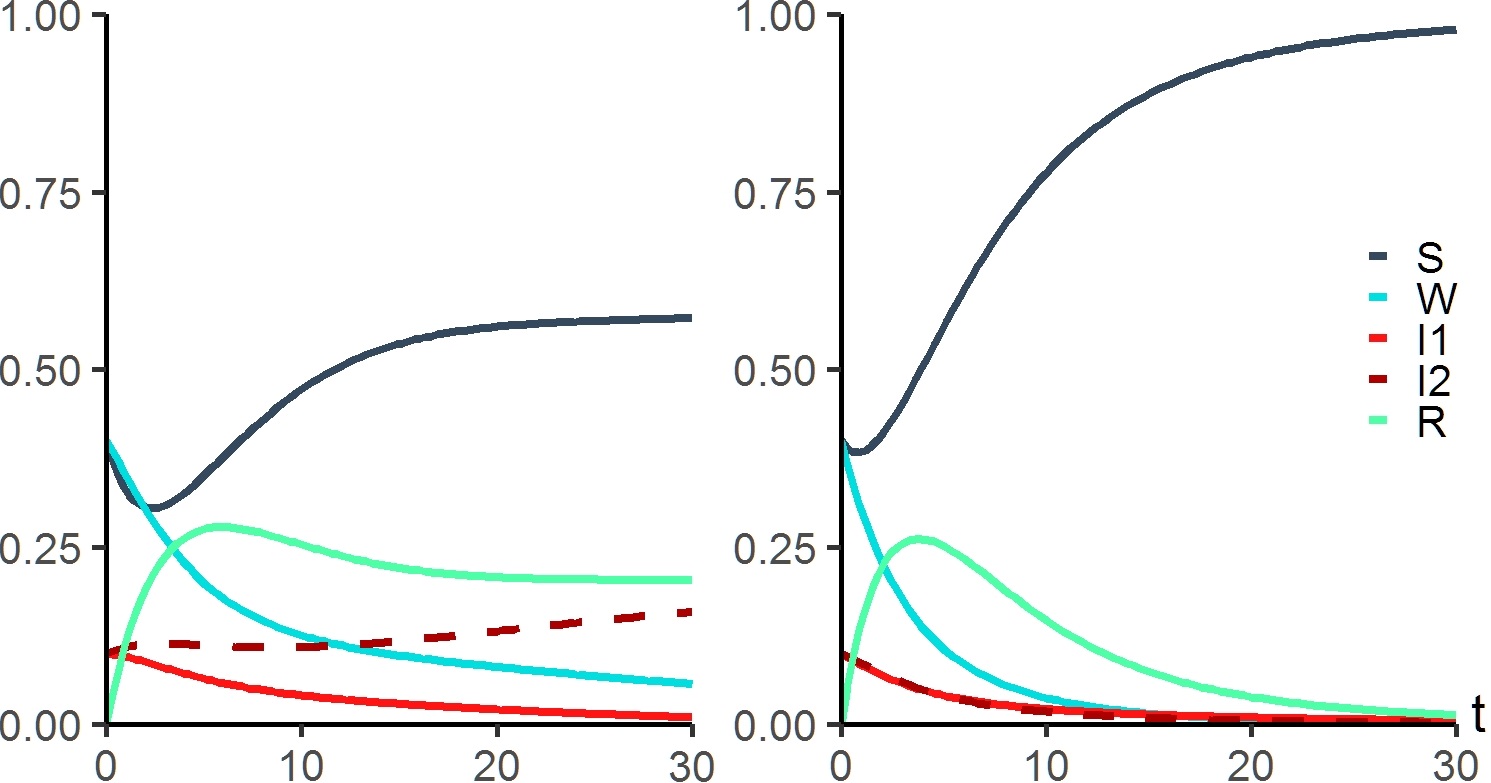
Let be a concave functions (), then according to (10) Hamiltonian is a convex function of . There could be two different options for that maximimize the Hamiltonian. If or , then optimal control – (Fig. 3 (right)), otherwise – (Fig. 3 (left)). For , the optimal control parameters are defined as follows:

| (22) |
2.5.2 Functions are strictly convex
Let be a strictly convex functions (), then Hamiltonian is concave function. Consider the following derivative:
| (23) |
where , . There could be three different types of points at which the Hamiltonian reaches its maximum (Fig. 4). To find them, we need to consider the derivatives of the Hamiltonian at and . If the derivatives (23) at are non-increasing (), then the value of the control that maximizes the Hamiltonian is less than 0, and according to our restrictions () optimal control will be equal to 0 (Fig. 4a). If the derivatives at are increasing (), it means that the value of the control that maximizes the Hamiltonian is greater than 1. Hence the optimal control will be equal to 1 (Fig. 4c), otherwise, we can find such value (Fig. 4b):

| (24) |
Functions , , are continuous at all In this case is strictly convex and is strictly increasing functions, so . Thus there exist points and so that conditions (24) are satisfied, and according to are decreasing functions.
After obtaining the optimal control and , we need to sort all infected nodes by the number of neighbors and treat them in order, starting with the first one on the list. Similar procedure is used to find the number of susceptible nodes, among which it is necessary to disseminate information about virus attacks, using the structure of the .
3 SWIRS model on meta-population network
The clustering of the nodes in the network can be considered as a natural extension of the SWIRS model from Section 2. We assume that all nodes inside the one cluster follow the same behavioral rules. However, the infection can be transferred among clusters. For this reason, we consider a case of a network with nodes, which can be divided into several clusters. Here, the matrix is the adjacency matrix of the first level of SWIRS model, where information about possible consequences of malware attacks is spreading, and is the adjacency matrix of the second level, where special antivirus patches are applied. Denote as the probability that a node from cluster of size and a node from a cluster of size change their states from to at every time instant. The probability that a susceptible node from cluster will be infected due to the contact with a node from a cluster , infected by virus is equal to . A warned node from cluster will be infected by virus through the contact with the node from a cluster with probability .
Vector defines the proportions distribution of being in each of the states for the cluster at . For any , the sum of the probabilities for any node is equal to . All other parameters in the system remain the same as in Section 3.1. This simultaneous process of information spreading and patching is described by a system of nonlinear differential equations:
| (25) |
where defines the sum from to . Initial states are , for all clusters .
The aggregated system costs on the time interval are defined as , where
| (26) |
and the optimal control problem is to minimize these costs, i.e.,
We focus on a case when both malware can cause extreme damages, and there is a need to lock down the entire system to prevent future destruction. To avoid this lockdown or other expensive security activity, we have to construct a constant control such that any malware will be instantly eliminated, even though the time when the viruses attack the system cannot be precisely identified. We assume that
We have to define the condition for which remains system in disease free state with minimum costs. We assume that . The initial state of the system is the equilibrium point from the Section 3.2. (25) can be reformulated as:
| (27) |
It is assumed that viruses can infect only one node at one time moment, then the system can be transformed in the following way:
| (28) |
where is a node which was infected by a virus. Inequalities (28) can be rewritten as
| (29) |
We find control strategies that maintain the disease free state in the the worst case of epidemics. This value provides an estimation on system costs when on the time interval . Summing the control parameters gives:
| (30) |
where is the control of a type in a cluster at time . As a result, we obtain
| (31) |
4 Numerical Experiments
In this section, we present numerical case studies to corroborate our results. For the experiments, we use the following costs functions: infection costs – and ; treatment costs – , ; vaccination cost – ; and utility functions are and . The time interval in the first two experiments is equal to [0,20].

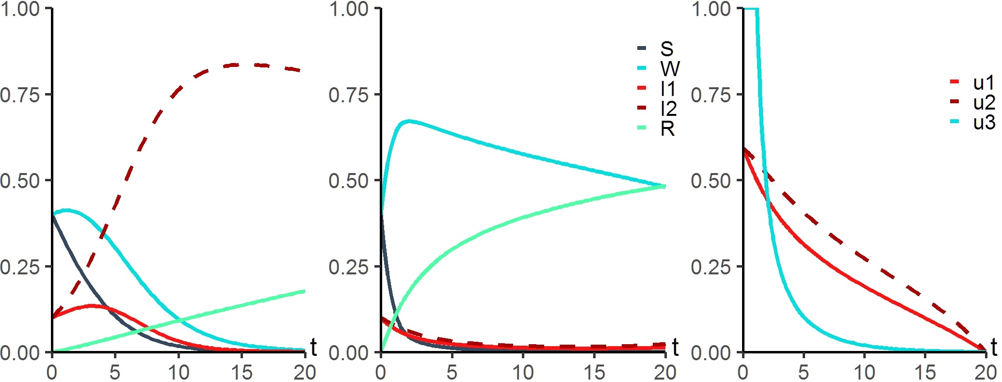
Experiment I shows the behaviour of the SWIRS-model in two different cases: controlled and uncontrolled ones (Fig. 5). In the uncontrolled cases, at the majority of nodes are infected by virus (). The values of the functionals are equal to and . After the treatment and information dissemination about possible epidemic outbreaks, all infected nodes are cured. Here, all nodes are in the disease free state (, , ) and values of the functionals are equal to and . Comparing the aggregated costs in the uncontrolled case () and the controlled case (), we can see that information spreading and applied treatment are beneficial.
Fig. 6 represents the dependence of the total number of infected nodes throughout the epidemic process on the parameters and in the uncontrolled (left) and the controlled (right) cases, where

In experiment II, we present the structure of the optimal control policies for the SWIR-model, when . In this case, after the treatment, the recovered node will not be infected again during the contacts with infected nodes. The final state of the system is (). The aggregated system costs in the uncontrolled case are ( and ). In the controlled case, the aggregated system costs reduced to ( and ).
Experiment III presents the SWIRS model on a meta-population network, the behavior of the system (25) in two different clusters is represented in Fig. 8.
| (32) |

Initial parameters are and . Matrices A=B show the strong connections between these clusters, hence the epidemics which has been started in the first cluster continues in the second one. Final states are and .
5 Conclusions
This paper presents a modified Susceptible-Warned- Infected-Recovered-Susceptible (SWIRS) model of simultaneous spreading of the virus protection information and the malware over a large population of nodes. We have investigated the stability of SWIR and SWIRS epidemic models with two coexisting malware types for heterogeneous populations. We have obtained the structure of the optimal control as well as the properties of feasible controls for a special class of cost functions. Numerical examples have been used to corroborate the results. We would further explore the stability properties of the epidemic process under optimal control. Another future work includes the extension of the SWIR model to an epidemic model over complex networks with different topologies.
6 Acknowledgement
The research has been partially supported by the RSF grant No. 16-19-10609, U.S. National Science Foundation Awards ECCS-1847056, CNS-1544782, and SES-1541164, and grant W911NF-19-1-0041 from U.S. Army Research Office (ARO).
References
- Allen (2008) Allen L. J. S. An introduction to stochastic epidemic models. Mathematical epidemiology, Springer. pp. 81-130, 2008.
- Altman (2011) Altman E., Khouzani M., Sarkar S. Optimal control of epidemic evolution. Proceedings of INFOCOM., pp. 1683–1691, 2011.
- Altman (2019) Altman E., Avrachenkov K., De Pellegrini F., El-Azouzi R., Wang H. Multilevel Strategic Interaction Game Models for Complex Networks. Springer Nature, Switzerland, 2019.
- Capasso (1993) Capasso V. Mathematical Structures of Epidemic Systems, Vol.97, 1993.
- Huang and Zhu (2019a) Huang Y., Zhu Q. A differential game approach to decentralized virus-resistant weight adaptation policy over complex networks. IEEE Transactions on Control of Network Systems, 2019.
- Huang and Zhu (2019b) Huang Y., Zhu Q. Achieving Social Optimum in Dynamic Weight Adaptation for Virus Mitigation: A Potential Differential Game Approach. Proc. of IFAC Workshop on Distributed Estimation and Control in Networked Systems (NECSYS 2019), IFAC-PapersOnLine, 52(20), pp.241–246, 2019.
- Farooq and Zhu (2017) Farooq M.J., Zhu Q., 2017, Secure and reconfigurable network design for critical information dissemination in the internet of battlefield things (IoBT). 15th International Symposium on Modeling and Optimization in Mobile, Ad Hoc, and Wireless Networks (WiOpt), pp. 1–8, 2017.
- Farooq and Zhu (2019) Farooq M.J., Zhu Q. Modeling, analysis, and mitigation of dynamic botnet formation in wireless IoT networks. IEEE Transactions on Information Forensics and Security, Vol.14, No. 9, pp. 2412–2426, 2019.
- Fedyanin (2011) Fedyanin D.N., Chkhartishvili A.G. On a model of informational control in social networks. Automation and Remote Control, Vol. 72, No. 10. p. 2181–2187., 2011.
- Luo (2009) Luo X., Liao Q. Ransomware: A new cyber hijacking threat to enterprises. Handbook of research on information security and assurance. pp. 1-6, 2009
- Mieghem (2009) Mieghem P. V., Omic J., Kooij R. Virus spread in Networks. IEEE/ACM Transactions on Networking. Vol. 17, No. 1. pp. 1-14, 2009.
- Moon (2019) Moon A. S., Sahneh F.D., Scoglio C. Generalized group-based epidemic model for spreading processes on networks: GgroupEM, arXiv:1908.06057, Physics and Society (physics.soc-ph), 2019.
- Moore (2002) Moore D., Shannon C. Code-Red: a Case Study on the Spread and Victims of an Internet Worm. Proceedings of the 2002 ACM SICGOMM Internet Measurement Workshop. 273–284, 2002.
- Newman (2016) Newman L. H. What we know about Friday’s massive east coast Internet outage. Wired Magazine, Oct. 21, 2016, https://www.wired.com/2016/10/internet-outage-ddos-dns-dyn/
- Pontryagin (1962) Pontryagin L., Boltyanskii V., Gamkrelidze R., Mishchenko E. The Mathematical Theory of Optimal Processes. Russia: Interscience, 1962.
- Sharma (2015) Sharma S., Samanta G. P. Stability analysis and optimal control of an epidemic model with vaccination. International Journal of Biomathematics, 2015. Vol. 8, No. 3, P. 28, 2015.
- Sahneh (2013) Sahneh F.D., Scoglio C., and Mieghem P. V. Generalized epidemic meanfield model for spreading processes over multilayer complex networks. IEEE/ACM Transactions on Networking. Vol. 21, No. 5. pp. 1609-1620, 2013.
- Taynitskiy (2015) Taynitskiy V., Gubar E., Zhitkova E. Structure of optimal control in the model of propagation of two malicious softwares. Proc. of Int. conf. ”Stability and Control Processes” in memory of V.I. Zubov (SCP)., 261—264, 2015.
- Taynitskiy (2017) Taynitskiy V., Gubar E., Zhu Q. Optimal Impulsive Control of Epidemic Spreading of Heterogeneous Malware. IFAC-PapersOnLine. Vol.50 , No.1, pp.15038 – 15043, 2017.
- Taynitskiy (2017) Taynitskiy V., Gubar E., Zhu Q. Optimal Security Policy for Protection Against Heterogeneous Malware. Static and Dynamic Game Theory: Foundations and Applications. pp. 199–209, 2017.
- Taynitskiy (2018) Taynitskiy V., Gubar E., Zhu Q. Optimal Control of Heterogeneous Mutating Viruses. Games, Volume 9, Issue 4, Article number 103, 2018.
- Vespignani (2015) Vespignani A., Pastor-Satorras R., Van Mieghem M, Castellano C. Epidemic processes in complex networks. Rev. Mod. Phys., Vol. 87, No. 925, 2015.
- Wang (2017) Wang W., Tang M., Stanley H.E., Braunstein L. A. Unification of theoretical approaches for epidemic spreading in complex networks. Reports on Progress in Physics. Vol. 80, No.3. pp. 1–16, 2017.
- Wu (2013) Wu Q., Small M., Liu H. Superinfection Behaviors on Scale-Free Networks with Competing Strains. Journal of Nonlinear Science., 23, 113—127, 2013.
- Zuzek (2015) Zuzek L. G. A., Stanley H. E., Braunstein L. A. Epidemic Model with Isolation in Multilayer Networks. Sci. Rep. 5, 12151; doi: 10.1038/srep12151, 2015.