Introduction to Random fields
March 1, 2007
General linear models (GLM) are often constructed and used in statistical inference at the voxel level in brain imaging. In this paper, we explore the basics of random fields and the multiple comparisons on the random fields, which are necessary to properly threshold statistical maps for the whole image at specific statistical significance level. The multiple comparisons are crucial in determining overall statistical significance in correlated test statistics over the whole brain. In practice, - or -statistics in adjacent voxels are correlated. So there is the problem of multiple comparisons, which we have simply neglected up to now. For multiple comparisons that account for spatially correlated test statistics, various methods were proposed: Bonferroni correction, random field theory (Worsley 1994; Worsley, Marrett, Neelin, Vandal, Friston & Evans 1996), false discovery rates (Benjamini & Hochberg 1995; Benjamini & Yekutieli 2001; Genovese et al. 2002) and permutation tests (Nichols & Holmes 2002). Among them, we will explore the random field approach.
1 Introduction
Suppose we measure temperature at position and time in a classroom . Since every measurement will be error-prone, we model the temperature as
where is the unknown signal and is the measurement error. The measurement error can be modelled as a random variable. So at each point , measurement error is a random variable. The collection of random variables
is called a stochastic process. The generalization of a continuous stochastic process defined in to a higher dimensional abstract space indexed by a spatial variable is called a random field. For an introduction to random fields, see Adler & Taylor 2007, Dougherty 1999 and Yaglom 1987. A formal measure theoretic definition can be found in Adler 1981 and Gikhman & Skorokhod 1996.
In brain imaging studies, it is necessary to model measurements at each voxel as a random field. For instance, in the deformation-based morphometry (DBM), deformation fields are usually modeled as continuous random fields (Chung et al. 2001). In the random field theory as used in (Worsley 1994; Worsley, Marrett, Neelin, Vandal, Friston & Evans 1996), measurement at voxel position is modeled as
where is the unknown signal to be estimated and is the measurement error. The measurement error at each fixed can be modeled as a random variable. Then the collection of random variables is called a stochastic process or random field. The more precise measure-theoretic definition can be found in (Adler & Taylor 2007). Random field modeling can be done beyond the usual Euclidean space to curved cortical and subcortical manifolds (Joshi 1998; Chung et al. 2003).
2 Random Fields
We start with defining a random field more formally using random variables. Our construction follows from Adler 1981.
Definition 1
Given a probability space, a random field defined in is a function such that for every fixed , is a random variable on the probability space.
Definition 2
The covariance function of a random field is defined as
Consider a random field . If the joint distribution
is invariant under the translation
is said to be stationary or homogeneous. For a stationary random field , we can show
and subsequently
for some function . Although the converse is not always true, such a case is not often encountered in practical applications (Yaglom 1987) so we may equate the stationarity with the condition
A special case of stationary fields is an isotropic field which requires the covariance function to be rotation invariant, i.e.
for some function . is the geodesic distance in the underlying manifold.
2.1 Gaussian Fields
The most important class of random fields is Gaussian fields. A more rigorous treatment can be found in Adler & Taylor 2007. Let us start defining a multivariate normal distribution from a Gaussian random variable.
Definition 3
A random vector is multivariate normal if is Gaussian for every possible .
Then a Gaussian random field can be defined from a multivariate normal distribution.
Definition 4
A random field is a Gaussian random field if are multivariate normal for every .
An equivalent definition to Definition 4 is as follows.
Definition 5
is a Gaussian random field if the finite joint distribution
is a multivariate normal for every .
is a mean zero Gaussian field if for all . Because any mean zero multivariate normal distribution can be completely characterized by its covariance matrix, a mean zero Gaussian random field can be similarly determined by its covariance function . Two fields and are independent if and are independent for every and . For mean zero Gaussian fields and , they are independent if and only if the cross-covariance function
vanishes for all and .
Given two arbitrary mean zero Gaussian fields, is there mapping that makes them independent? Let be a vector field. Let be a constant matrix. Consider transformation and its covariance
Note that is symmetric and its diagonal terms are positive so it is a symmetric positive definite matrix so we have a singular value decomposition of the form where is an orthogonal matrix. Simply let and it should make the component of uncorrelated for all and . But they are still not independent.
The Gaussian white noise is a Gaussian random field with the Dirac-delta function as the covariance function. Note the Dirac delta function is defined as , and . Numerically we can simulate the Dirac delta function as the limit of the sequence of Gaussian kernel when . The Gaussian white noise is simulated as an independent and identical Gaussian random variable at each voxel.
2.2 Derivative of Gaussian Fields
Any linear operation on Gaussian fields is again Gaussian fields. Suppose be a collection of Gaussian random fields. Then . For given , we have again for all and . Therefore, forms an infinite-dimensional vector space. Not only the linear combination of Gaussian fields is again Gaussian but also the derivatives of Gaussian fields are Gaussian. To see this, we define the mean-square convergence.
Definition 6
A sequence of random fields , indexed by converges to as in mean-square if
We will denote the mean-square convergence using the usual limit notation:
The convergence in mean-square implies the convergence in mean. This can be seen from
Now let in mean square. Each term in the right hand side should also converges to zero proving the statement.
Now we define the derivative of field in mean square sense as
Note that if and are Gaussian random fields, is again Gaussian, and hence the limit on the right hand side is again Gaussian. If is the covariance function of the mean zero Gaussian field , the covariance function of its derivative field is given by
Given zero mean Gaussian field , the Hessian field of is given by
If we have mean zero Gaussian random variables if odd. Hence the expectation of the determinant of Hessian of a mean zero Gaussian field vanishes. For even and assuming isotropic covariance , i.e., stationarity, we can further simplify the expression.
2.3 Integration of Gaussian Fields
The integration of Gaussian fields is also Gaussian. To see this, define the integration of a random field as the limit of Riemann sum. Let be a partition of , i.e.
Let and be the volume of . Then we define the integration of field as
where the limit is taken as for all .
Multiple integration is defined similarly. When we integrate a Gaussian field, it is the limit of a linear combination of Gaussian random variables so it is again a Gaussian random variable. In general, any linear operation on Gaussian fields will result in a Gaussian field.
Let be a zero mean Gaussian fields in with covariance function . Let’s find the distribution of . Obviously this is a zero mean Gaussian random variable so we only need to find the second moment
2.4 , and Fields
We can use i.i.d. Gaussian fields to construct -, -, -fields, all of which are extensively studied in (Cao & Worsley 1999; Worsley et al. 2004; Worsley, Marrett, Neelin, Vandal, Friston & Evans 1996; Worsley 1994). The -field with degrees of freedom is defined as
where are independent, identically distributed Gaussian fields with zero mean and unit variance. Similarly, we can define and fields as well as Hotelling’s field. The Hotelling’s -statistic has been widely used in detecting morphological changes in deformation-based morphometry (Cao & Worsley 1999; Collins et al. 1998; Gaser et al. 1999; Joshi 1998; Thompson et al. 1997). In particular, (Cao & Worsley 1999) derived the excursion probability of the Hotelling’s -field and applied it to detect gender specific morphological differences.
3 Convolution on Random Fields
Consider the following integral
where is called the kernel of the integral. Define convolution between kernel and random field as the above integral.
Suppose the kernel to be isotropic probability density, i.e. and Further we may assume to be unimodal with some parameter such that
the Dirac-delta function. Since the Dirac-delta function satisfies
it can be easily seen that
3.1 Kernel smoothing estimator
Let The -dimensional isotropic Gaussian kernel is given by the products of -dimensional Gaussian kernel:
The isotropic kernel under linear transform changes the shape of the kernel to anisotropic kernel
Note the multivariate kernel is a probability distribution, i.e.,
is the Jacobian of the transformation that normalize the density. It is the distribution of -dimensional multivariate normal with the covariance matrix , i.e. . is also called the bandwidth matrix in the context of kernel smoothing and it measures the amount of smoothing. It can be shown that satisfy the definition of the Dirac-delta function as the eigenvalues of go to zero, i.e.
The limit of the sequence of the Gaussian kernels gives the Dirac-delta function and this is how we implement the Dirac-delta function in computer programs. From now on we let if all and if all .
Suppose we have an additive model
where is a mean zero random field and is an unknown signal. In image analysis, observations are so dense that we can take them to be continues functional data. Then the kernel smoothing estimator is given by
| (1) |
As goes to zero, we are smoothing less. To see this note that
From (1),
From the property of the Dirac-delta, as , converges to the true but unknown signal . So we can see that our kernel estimator becomes more unbiased as .
We can show that the estimator is a solution to a heat equation and the condition is equivalent to the steady state that is reached when we diffuse heat for infinite amount of time (Chung 2012).
Other properties of kernel smoothing estimator is as follows. Assuming ,
| (2) |
Similarly we can bound from below so that
| (3) |
Inequality (3) implies that smoothed signal will be smaller than the maximum and larger than the minimum of the signal in average. Other interesting property is
| (4) | |||||
| (5) |
Thus we have
If is a probability such as the transition probability in Brownian motion, it implies that the total probability is conserved even after smoothing.
Let be the covariance function of field with . It is trivially
the covariance function of . Then we can show that the covariance function of the kernel smoother can be shown to be
| (6) |
4 Numerical Simulation of Gaussian Fields
For the random field theory based multiple correction to work, it is necessary to have smooth images. In this section, we show how to simulate smooth Gaussian fields by performing Gaussian kernel smoothing on white noise. This is the easiest way of simulating Gaussian fields.
White noise is defined as a random field whose covariance function is proportional to the Dirac-delta function , i.e.
For instance, me may take , the limit of the usual isotropic Gaussian kernel. White noise is usually characterized via generalized functions.
One example of white noise is the generalized derivative of Brownian motion (Wiener process) called white Gaussian noise.
Definition 7
Brownian motion (Wiener process) is zero mean Gaussian field with covariance function
Following Definition 7, we can show by taking in the covariance function and by letting in the variance. The increments of Wiener processes in nonoverlapping intervals are independent identically distributed (iid) Gaussian. Further the paths of the Wiener process is continous in the Kolmogorov sense while it is not differentiable. For a different but identical canonical construction of Brownian motion, see (Øksendal 2010). Higher dimensional Brownian motion can be generalized by taking each component of vector fields to be i.i.d. Brownian motion.

Although the path of Wiener process is not differentiable, we can define the generalized derivative via integration by parts with a smooth function called a test function in the following way
Taking the expectation on both sides we have
It should be true for all smooth so . Further it can be shown that the covariance function of process .
The Gaussian white noise can be used to construct smooth Gaussian random fields of the form
where is a Gaussian kernel. Since Brownian motion is zero mean Gaussian process, is obviously zero mean field with the covariance function
| (7) | |||||
| (8) |
The case when is an isotropic Gaussian kernel was investigated by D.O. Siegmund and K.J. Worsley with respect to optimal filtering in scale space theory (Siegmund & Worsley 1996).
In numerical implementation, we use the discrete white Gaussian noise which is simply a Gaussian random variable.
Example 1
Let be a discrete version of white Gaussian noise given by
where i.i.d. . Note that
| (9) |
The collection of random variables forms a multivariate normal at arbitrary points . Hence the field is a Gaussian field.
The covariance function of the field 9 is given by
| (10) | |||||
| (11) |
As usual we may take to be a Gaussian kernel. Let us simulate some Gaussian fields.
Example 2
The unknown signal is assumed to be and white noise error which is shown in the top left of Figure 1. Then iteratively more smooth version of Gaussian random fields are constructed by
w=normrnd(0,0.4,101,101);
smooth_w=w;
for i=1:10
  smooth_w=conv2(smooth_w,K,’same’);
  figure;imagesc(smooth_w);colorbar;
end;
with kernel weight K.
5 Statistical Inference on Fields
Given functional measurement , we have model
where is unknown signal and is a zero mean unit variance Gaussian field. We assume . In brain imaging, one of the most important problems is that of signal detection, which can be stated as the problem of identifying the regions of statistical significance. So it can be formulated as an inference problem
Let
at a fixed point . Then the null hypothesis is a collection of multiple hypotheses over all . Therefore, we have
We may assume that is the region of interest consisting of the finite number of voxels. We also have the corresponding point-wise alternate hypothesis
and the alternate hypothesis is constructed as
If we use -statistic as a test statistic, for instance, we will reject each if for some threshold . So at each fixed , for level test, we need to have . However, if we threshold at , of observations are false positives. Note that the false positives are pixels where we are incorrectly rejecting when it is actually true. However, these are the false positives related to testing . For determining the true false positives associated with testing , we need to account for multiple comparisons.
Definition 8
The type-I error is the probability of rejecting the null hypothesis (there is no signal) when the alternate hypothesis (there is a signal) is true.
The type-I error is also called the family-wise error rate (FWER) and given by
| (12) | |||||
Unfortunately, is correlated over and it makes the
computation of type-I error almost intractable for random fields
other than Gaussian.
5.1 Bonferroni Correction
One standard method for dealing with multiple comparisons is to use the Bonferroni correction. Note that the probability measure is additive so that for any event , we have
This inequality is called Bonferroni inequality and it has been used in the construction of simultaneous confidence intervals and multiple comparisons when the number of hypotheses are small. From (12), we have
| (13) | |||||
| (14) |
So by controlling each type-I error separately at
we can construct the correct level test. Here is the number of voxels.
The problem with the Bonferroni correction is that it is too conservative. The Bonferroni inequality (14) becomes exact when the measurements across voxels are all independent, which is unrealistic. Since the measurements are expected to be strongly correlated across voxels, we have highly correlated statistics. So in a sense, we have a less number of comparisons to make.
Let us illustrate the Bonferroni correction procedure using MATLAB. Consider image of standard normal random variables (Figure 2). The threshold corresponding to the significance is 1.64.

Y=normrnd(0,1,100,100);
figure; imagesc(Y); colorbar; colormap(’hot’)

norminv(0.95,0,1)

ans =

    1.6449

[Yl, Yh] = threshold_image(Y, 1.64);
figure; imagesc(Yh); colormap(’hot’); colorbar;
By thresholding the image at 1.64, we obtain approximately about 5 of pixels as false positives. To account for the false positives, we perform the Bonferroni correction. For image of size , there are pixels. Therefore, is the corresponding point-wise -value and the corresponding threshold is 4.42. In this example, there is no pixel that is higher than 4.42 so we are not detecting any false positives as expected.
n=100*100;
size(find(reshape(Y,n,1)>=1.64),1)/n
norminv(1-0.05/10000,0,1)

ans =

    4.4172
5.2 Rice Formula
We can obtain a less conservative estimate for (12) using the random field theory. Assuming , we have
| (15) | |||||
In order to construct the -level test corresponding to , we need to know the distribution of the supremum of the field . The corresponding -value based on the supremum of the field, i.e. , is called the corrected -value to distinguish it from the usual -value obtained from the statistic . Note that the p-value is the smallest -level at which the null hypothesis is rejected.
Analytically computing the exact distribution of the supremum of random fields is hard. If we denote and to be the cumulative distribution of , for the given , we can compuate . Then the region of statistically significant signal is localized as .
The distribution of supremum of Brownian motion is somewhat simple due to its independent increment properties. However, for smooth random fields, it is not so straightforward. Read (Adler 2000) for an overview of computing the distribution of the supremum of smooth fields.
Consider 1D smooth stationary Gaussian random process . Let to be the number of times crosses over from below (called upcrossing) in . Then we have
If is the covariance function of the field , we have
It can be shown that from Rice formula (Adler et al. 1993; Rice 1944),
Also note that
where is the cumulative distribution function of the standard normal. Then from the inequality that bounds the cumulative distribution of the standard normal (Feller 1968), we have
So
for some and . In fact we can show that
5.3 Poisson Clumping Heuristic
To extend the Rice formula to a higher dimension, we need a different mathematical machinery. For this method to work, the random field needs to be sufficiently smooth and isotropic. The smoothness of a random field corresponds to the random field being differentiable. There are very few cases for which exact formulas for the excursion probability (15) are known (Adler 1990). For this reason, approximating the excursion probability is necessary for most cases.
From the Poisson clumping heuristic (Aldous 1989),
where is the Lebesgue measure of a set and the random set
is called the excursion set above the threshold . This approximation involves unknown , which is the mean clump size of the excursion set. The distribution of has been estimated for the case of Gaussian (Aldous 1989), and fields (Cao 1999) but for general random fields, no approximation is available yet.
6 Expected Euler Characteristics
An alternate approximation to the supremum distribution based on the expected Euler characteristic (EC) of is also available. The Euler characteristic approach reformulates the geometric problem as a topological problem. Read (Adler 1981; Cao & Worsley 2001; Taylor & Worsley 2007; Worsley 2003) for an overview of the Euler characteristic method.
For sufficiently high threshold , it is known that
| (16) |
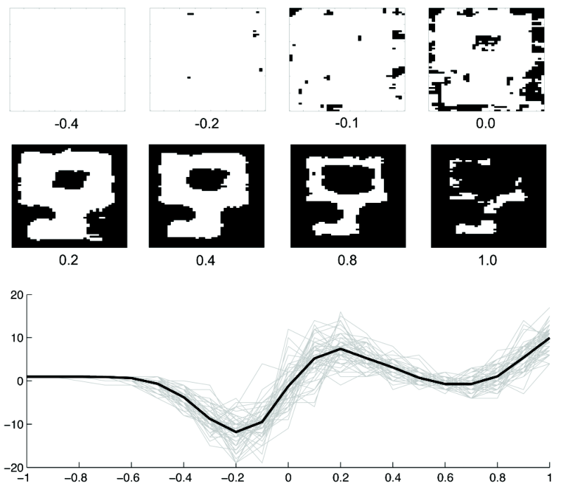
where is the -th Minkowski functional or intrinsic volume of and is the -th Euler characteristic (EC) density of (Worsley et al. 1998). For details on intrinsic volume, read (Schmidt & Spodarev 2005). The expansion (16) also holds for non-isotropic fields but we will not pursue it any further. Compared to other approximation methods such as the Poisson clump heuristic and the tube formulae, the advantage of using the Euler characteristic formulation is that a simple exact expression can be found for . Figure 3 and Figure 4 show how and change as the threshold increases for a simple binary object with a hole.
6.1 Intrinsic Volumes
The -th intrinsic volume of is a generalization of -dimensional volume. Note that is the Euler characteristic of . is the volume of while is half the surface area of . There are various techniques for computing the intrinsic volume (Taylor & Worsley 2007). The methods depend on the smoothness of the underlying manifold . For a solid sphere with radius , the intrinsic volumes are
For a 3D box of size , the intrinsic volumes are
In general, the intrinsic volume can be given in terms of a curvature matrix. Let be the curvature matrix of and be the sum of the determinant of all principal minors of . For the Minkowski functional is defined as
and , the Lebesgue measure of .

For irregular jagged shapes such as the 2D corpus callosum shape , the intrinsic volume can be estimated in the following fashion (Worsley, Marrett, Neelin & Evans 1996; Chung et al. 2004). Treating pixels inside as points on a lattice, let be the number of vertices that forms the corners of pixels, be the number of edges connecting each adjacent lattice points and be the number of faces formed by four connected edges. We assume the distance between the adjacent lattice points is in all directions. Then
To find the number of edges and pixels contained in , we start from an initial face (pixel) somewhere in the corpus callosum and add one face at a time while counting the additional edges and faces. In this fashion, we can grow a graph that will eventually contains all the pixels that form the corpus callosum. A numerical method for computing the intrinsic volume for jagged irregular shapes has been implemented in FMRISTAT package (www.math.mcgill.ca/keith/fmristat).
6.2 Euler Characteristic Density
The -th EC-density is given by
where dot notation indicates partial differentiation with respect to the first components. The subscript represents the first components of . Computation of the conditional expectation is nontrivial other than for Gaussian fields. For zero mean and unit variance Gaussian field , we have for instance
where measures the smoothness of fields, defined as the variance of the derivative of component of . The exact expression for the EC density is available for other random fields such as fields (Worsley 1994), Hotelling’s fields (Cao & Worsley 1999) and scale-space random fields (Siegmund & Worsley 1996). In each case, the EC density is proportional to and it changes depending on the smoothness of the field.
If are i.i.d. stationary zero mean unit variance Gaussian fields. Then -field with and degrees of freedom is given by
To avoid singularity, we need to assume the total degrees of freedom to be sufficiently larger than the dimension of space (Worsley 1994). The EC-density for -field is then given by
If the random field is given as the convolution of a smooth kernel with a white Gaussian noise (Siegmund & Worsley 1996; Worsley et al. 1992), the covariance matrix of is given by
Applying it to a Gaussian kernel gives
In terms of FWHM of the kernel ,
6.3 Numerical Implementation of Euler Characteristics
In this section, we show how to compute the expected Euler characteristic in MATLAB. The presented routine can be used in estimating the excursion probability numerically. Consider a 2D binary object (Figure 3), which is stored as a 2D image toy-key.tif. After loading the image using imread, we perform scaling on image intensity values so that it becomes a binary object. The Euler characteristic of the binary object is then computed using bweuler.
I=imread(’toy-key.tif’);
I= imresize(I,.1, ’nearest’);
I=(max(max(I))-I);
I=I/max(max(I));
I=double(I);
figure;imagesc(I); colormap(’hot’)
eul = bweuler(I)

eul =

     0
Since there is a hole in the object, the Euler characteristic is 0. We will add Gaussian white noise to the binary object and smooth out with FWHM of 10 using gaussblur. The resulting image is a Gaussian random field with sufficient smoothness. The smoothed image is stored as smooth and displayed in Figure 3.
e=normrnd(0,1, 60, 37);
Y=I + e;
figure;imagesc(Y); colorbar; colormap(’hot’)
smooth = gaussblur(Y,10);
figure;imagesc(smooth);colorbar; colormap(’hot’);
At each threshold h between -1 and 1, we threshold smooth and store it as a new variable excursion. Then compute the Euler characteristic of excursion. For computing the mean of the Euler characteristic, we simulated Gaussian random fields 50 times using the for-loop.
figure;
eulsum=zeros(1,21);
for k=1:50
    Y=I+ normrnd(0,1,60,37);
    smooth = gaussblur(Y,10);
    eul=[];
    j=1;
    for h=-1:0.1:1
        [Yl, Yh] = threshold_image(smooth, h);
        Yh=reshape(Yh,60*37,1);
        excursion=zeros(60*37,1);
        excursion(find(Yh>h))=1;
        excursion=reshape(excursion, 60, 37);
        eul(j) = bweuler(excursion);
        j=j+1;
    end;
    hold on; plot(-1:0.1:1, eul, ’Color’, [0.7 0.7 0.7])
    eulsum=eulsum+eul;
end;
hold on; plot(-1:0.1:1, eulsum/50, ’Color’, ’k’, ’LineWidth’,2)
References
- (1)
- Adler (1981) Adler, R. (1981), The Geometry of Random Fields, John Wiley Sons.
- Adler (1990) Adler, R. (1990), An Introduction to Continuity, Extrema, and Related Topics for General Gaussian Processes, IMS, Hayward, CA.
- Adler (2000) Adler, R. (2000), ‘On excursion sets, tube formulas and maxima of random fields’, Annals of Applied Probability 10, 1–74.
- Adler et al. (1993) Adler, R., Samorodnitsky, G. & Gadrich, T. (1993), ‘The expected number of level crossings for stationary, harmonisable, symmetric, stable processes’, The Annals of Applied Probability 3, 553–575.
- Adler & Taylor (2007) Adler, R. & Taylor, J. (2007), Random Fields and Geometry, Springer Verlag.
- Aldous (1989) Aldous, D. (1989), Probability Approximations via the Poisson Clumping Heuristic, Springer-Verlag, New York.
- Benjamini & Hochberg (1995) Benjamini, Y. & Hochberg, Y. (1995), ‘Controlling the false discovery rate: A practical and powerful approach to multiple testing’, Journal of Royal Statistical Society, Series. B 57, 289–300.
- Benjamini & Yekutieli (2001) Benjamini, Y. & Yekutieli, D. (2001), ‘The control of the false discovery rate in multiple testing under dependency’, Annals of Statistics 29, 1165–1188.
- Cao (1999) Cao, J. (1999), ‘The size of the connected components of excursion sets of , and fields’, Advances in Applied Probability 31, 579–595.
- Cao & Worsley (1999) Cao, J. & Worsley, K. (1999), ‘The detection of local shape changes via the geometry of Hotelling’s T2 fields’, Annals of Statistics 27, 925–942.
- Cao & Worsley (2001) Cao, J. & Worsley, K. (2001), ‘Applications of random fields in human brain mapping’, Spatial Statistics: Methodological Aspects and Applications 159, 170–182.
- Chung (2012) Chung, M. (2012), Computational Neuroanatomy: The Methods, World Scientific, Singapore.
- Chung et al. (2004) Chung, M., Dalton, K., Alexander, A. & Davidson, R. (2004), ‘Less white matter concentration in autism: 2D voxel-based morphometry’, NeuroImage 23, 242–251.
- Chung et al. (2001) Chung, M., Worsley, K., Paus, T., Cherif, D., Collins, C., Giedd, J., Rapoport, J. & Evans, A. (2001), ‘A unified statistical approach to deformation-based morphometry’, NeuroImage 14, 595–606.
- Chung et al. (2003) Chung, M., Worsley, K., Robbins, S., Paus, T., Taylor, J., Giedd, J., Rapoport, J. & Evans, A. (2003), ‘Deformation-based surface morphometry applied to gray matter deformation’, NeuroImage 18, 198–213.
- Collins et al. (1998) Collins, D., Paus, T., Zijdenbos, A., Worsley, K., Blumenthal, J., Giedd, J., Rapoport, J. & Evans, A. (1998), ‘Age related changes in the shape of temporal and frontal lobes: An mri study of children and adolescents’, Soc. Neurosci. Abstr. 24, 304.
- Dougherty (1999) Dougherty, E. (1999), Random Processes for Image and Signal Processing, IEEE Press.
- Feller (1968) Feller, W. (1968), Introduction to probability theory and its applications, Wiley, New York.
- Gaser et al. (1999) Gaser, C., Volz, H.-P., Kiebel, S., Riehemann, S. & Sauer, H. (1999), ‘Detecting structural changes in whole brain based on nonlinear deformations - Application to schizophrenia research’, NeuroImage 10, 107–113.
- Genovese et al. (2002) Genovese, C., Lazar, N. & Nichols, T. (2002), ‘Thresholding of statistical maps in functional neuroimaging using the false discovery rate’, NeuroImage 15, 870–878.
- Gikhman & Skorokhod (1996) Gikhman, I. & Skorokhod, A. (1996), Introduction to the theory of random processes, Courier Dover Publications.
- Joshi (1998) Joshi, S. (1998), Large Deformation Diffeomorphisms and Gaussian Random Fields for Statistical Characterization of Brain Sub-Manifolds, PhD thesis, Washington University, St. Louis.
- Nichols & Holmes (2002) Nichols, T. & Holmes, A. (2002), ‘Nonparametric permutation tests for functional neuroimaging: A primer with examples’, Human Brain Mapping 15, 1–25.
- Øksendal (2010) Øksendal, B. (2010), Stochastic Differential Equations: An Introduction with Applications, Springer.
- Rice (1944) Rice, S. (1944), ‘Mathematical analysis of random noise’, Bell System Tech. J 23, 282–332.
- Schmidt & Spodarev (2005) Schmidt, V. & Spodarev, E. (2005), ‘Joint estimators for the specific intrinsic volumes of stationary random sets’, Stochastic Processes and their Applications 115, 959–981.
- Siegmund & Worsley (1996) Siegmund, D. & Worsley, K. (1996), ‘Testing for a signal with unknown location and scale in a stationary gaussian random field’, Annals of Statistics 23, 608–639.
- Taylor & Worsley (2007) Taylor, J. & Worsley, K. (2007), ‘Detecting sparse signals in random fields, with an application to brain mapping’, Journal of the American Statistical Association 102, 913–928.
- Thompson et al. (1997) Thompson, P., MacDonald, D., Mega, M., Holmes, C., Evans, A. & Toga, A. (1997), ‘Detection and mapping of abnormal brain structure with a probabilistic atlas of cortical surfaces’, Journal of Computer Assisted Tomography 21, 567–581.
- Worsley (1994) Worsley, K. (1994), ‘Local maxima and the expected Euler characteristic of excursion sets of , and fields.’, Advances in Applied Probability 26, 13–42.
- Worsley (2003) Worsley, K. (2003), ‘Detecting activation in fMRI data.’, Statistical Methods in Medical Research. 12, 401–418.
- Worsley et al. (1998) Worsley, K., Cao, J., Paus, T., Petrides, M. & Evans, A. (1998), ‘Applications of random field theory to functional connectivity’, Human Brain Mapping 6, 364–7.
- Worsley et al. (1992) Worsley, K., Evans, A., Marrett, S. & Neelin, P. (1992), ‘A three-dimensional statistical analysis for CBF activation studies in human brain’, Journal of Cerebral Blood Flow and Metabolism 12, 900–918.
- Worsley, Marrett, Neelin & Evans (1996) Worsley, K., Marrett, S., Neelin, P. & Evans, A. (1996), ‘Searching scale space for activation in pet images’, Human Brain Mapping 4, 74–90.
- Worsley, Marrett, Neelin, Vandal, Friston & Evans (1996) Worsley, K., Marrett, S., Neelin, P., Vandal, A., Friston, K. & Evans, A. (1996), ‘A unified statistical approach for determining significant signals in images of cerebral activation’, Human Brain Mapping 4, 58–73.
- Worsley et al. (2004) Worsley, K., Taylor, J., Tomaiuolo, F. & Lerch, J. (2004), ‘Unified univariate and multivariate random field theory’, NeuroImage 23, S189–195.
- Yaglom (1987) Yaglom, A. (1987), Correlation Theory of Stationary and Related Random Functions Vol. I: Basic Results, Springer-Verlag.