Decreasing Minimization on M-convex Sets:
Algorithms and Applications
Abstract
This paper is concerned with algorithms and applications of decreasing minimization on an M-convex set, which is the set of integral elements of an integral base-polyhedron. Based on a recent characterization of decreasingly minimal (dec-min) elements, we develop a strongly polynomial algorithm for computing a dec-min element of an M-convex set. The matroidal feature of the set of dec-min elements makes it possible to compute a minimum cost dec-min element, as well. Our second goal is to exhibit various applications in matroid and network optimization, resource allocation, and (hyper)graph orientation. We extend earlier results on semi-matchings to a large degree by developing a structural description of dec-min in-degree bounded orientations of a graph. This characterization gives rise to a strongly polynomial algorithm for finding a minimum edge-cost dec-min orientation.
Keywords: Network flows, Resource allocation, Graph orientation, Decreasing minimization,
M-convex set, Polynomial algorithm.
Mathematics Subject Classification (2010): 90C27, 05C, 68R10
Running head: Decreasing Minimization: Algorithms and Applications
1 Introduction
This paper is concerned with algorithms and applications of decreasing minimization on an M-convex set, which is the set of integral elements of an integral base-polyhedron. An element of a set of vectors, in general, is called decreasingly minimal (dec-min) if its largest component is as small as possible, within this, its second largest component is as small as possible, and so on. Decreasing minimization means the problem of finding a dec-min element of a given set of vectors (or even a cheapest dec-min element with respect to a given linear cost-function). When the given set of vectors consists of integral vectors, this problem is also referred to as discrete decreasing minimization. In the literature, typically the term lexicographic optimization is used, but we prefer “decreasing minimization” because we also consider its natural counterpart “increasing maximization,” and the use of these two symmetric terms seems more appropriate to distinguish the two related notions. An element of a set of vectors is called increasingly maximal (inc-max) if its smallest component is as large as possible, within this, its second smallest component is as large as possible, and so on.
In the companion paper [21], the present authors have investigated the structural aspects of the discrete decreasing minimization on an M-convex set. Among others, the dec-min elements are characterized as those admitting no local improvement, where the precise meaning of a local improvement is defined formally in term of “1-tightening step” in Section 2. It is also shown that an element of an M-convex set is decreasingly minimal precisely if it is a minimizer of the sum of the squared components.
As dual objects to dec-min elements, the notions of canonical chain, canonical partition of the ground-set, and essential-value sequence were defined, and the structure of the set of all dec-min elements is described in terms of these dual objects. (An equivalent definition of these notions is given in Section 2.2.) We emphasize that the role of these dual objects is not merely to help us fully understand the problem from its dual side. Beyond this, the dual characterization reveals the fundamental feature of the primal problem that the set of dec-min elements itself forms an M-convex set, and, in fact, a rather special one arising from a matroid by translation. In addition, these dual objects are inherent in computing a dec-min element in strongly polynomial time and indispensable for efficient computation of a minimum weight dec-min element, as well.
The first goal of this paper is to develop, on the basis of the above-mentioned structural characterizations, a strongly polynomial algorithm for computing a dec-min element as well as the canonical chain of a given M-convex set. The second goal is to exhibit several applications. For example, we prove a conjecture of Borradaile et al. [7] on dec-min strongly connected orientations of undirected graphs. Our general approach makes it possible to solve algorithmically even the minimum edge-cost dec-min orientation problem when upper and lower bounds are imposed on the in-degrees and the orientation is expected to be -edge-connected (or even -edge-connected). These orientation results form the basis of a major generalization of the so-called semi-matching problem initiated by Harvey et al. [31], which had been motivated by a resource allocation problem in computer science. Our approach is the first one that provides a strongly polynomial algorithm for the capacitated case, as well.
An algorithmic solution to a discrete counterpart of Megiddo’s lexicographic flow problem [43, 44] is also developed. Yet another application of the structural results of [21] gives rise to an extension of a result of Levin and Onn [42] on finding bases of a matroid on a ground-set with elements such that the degree-vector of the hypergraph formed by these bases is decreasingly minimal. Our approach generalizes this problem to the case when one has distinct matroids on .
The paper is organized as follows. Algorithms for computing a dec-min element and the canonical chain are given in Section 2. In Section 3, various kinds of applications are shown, including those to matroids, network flows, arborescences, and connectivity augmentations. Sections 4, 5, and 6 are devoted to detailed account of applications to graph orientation problems.
1.1 Notation and terminology
We continue to use notation and terminology introduced in [21], while some additional ones are given here. Let be a finite ground-set with elements. Two subsets and of are intersecting if , properly intersecting if none of , , and is empty, and crossing if none of , , , and is empty. For distinct elements of , a subset of containing but not is called a -set.
For a vector or a function , we define the set-function by . This is a modular function in the sense that holds for every .
For any integral polyhedron , we use the notation to denote the set of integral elements of , that is,
| (1.1) |
where may be pronounced “dotted .” The notation is intended to refer intuitively to the set of lattice points of .
For a set-function , we allow it to have value or . Unless otherwise stated, is assumed throughout. When is finite, the complementary function is defined by . Observe that the complementary function of is itself.
Let be a set-function with , for which is allowed but is not. The submodular inequality for subsets is defined by
| (1.2) |
We say that is (fully) submodular if this inequality holds for every pair of subsets with finite -values. When the submodular inequality is required only for intersecting (crossing) pairs of subsets, we say that is intersecting (crossing) submodular. A set-function is called (fully, intersecting, crossing) supermodular if is (fully, intersecting, crossing) submodular. It follows from the definitions that if is fully (or crossing) submodular with finite , then its complementary function is a fully (or crossing) supermodular function, while is not necessarily intersecting supermodular when is intersecting submodular.
For a (fully) submodular integer-valued set-function on with and finite , the base-polyhedron is defined by
| (1.3) |
which is a (possibly unbounded) integral polyhedron in . Section 14 of book [16] provides an overview of basic properties of base-polyhedra; see also the book of Schrijver [53]. For example, it is a basic property that is a non-empty integral polyhedron, and uniquely determines its defining (fully) submodular function , namely,
By convention, the empty set is also considered a base-polyhedron. A (fully) supermodular integer-valued set-function with and finite also defines an integral base-polyhedron by
| (1.4) |
since the complementary function of is fully submodular and . In discrete convex analysis [46, 47], the set of integral elements of an integral base-polyhedron is called an M-convex set.
We say that a submodular function and a supermodular function meet the cross-inequality for if
| (1.5) |
A pair of set-functions is called fully paramodular (or we say that is a strong pair) if is fully submodular, is fully supermodular, and the cross-inequality holds for every . For a strong pair , the polyhedron defined by
| (1.6) |
is called a generalized polymatroid (g-polymatroid, for short), while is called the border pair of . It is a basic fact [16] that is never empty. By convention, the empty set is also considered a g-polymatroid. Furthermore, a non-empty g-polymatroid uniquely determines its fully paramodular border pair, and is integral when and are integer-valued. Base-polyhedra are special g-polymatroids, namely, those for which , and every g-polymatroid arises from a base-polyhedron by projection along a single coordinate axis.
To prove theorems on base-polyhedra, it is much easier to work with base-polyhedra defined by fully sub- or supermodular functions. For applications, however, it is fundamentally important that weaker set-functions (e.g. intersecting, crossing or even weaker submodular functions) may also define base-polyhedra (or M-convex sets), as well as g-polymatroids. (We shall use this fact frequently in Sections 5 and 6.) For example, if is an integer-valued intersecting or crossing supermodular function, then can be proved to be an integral base-polyhedron (see, e.g. Theorem 15.3.4 in book [16]), which may, however, be empty. (This result, for example, underlies the fact that the in-degree vectors of -edge-connected orientations of a -edge-connected graph form an M-convex set.)
When is intersecting supermodular, is intersecting submodular, and the cross-inequality holds for properly intersecting pairs of subsets , we say that is a weak pair or intersecting paramodular. For such a border pair, is known to be a (possibly empty) g-polymatroid. It should be noted, that the (unique) fully paramodular border pair defining can be concretely expressed with the help of the weak pair , but this formula is quite complicated (see, Corollary 15.3.4 in book [16]).
It is a non-trivial task to characterize the situation when is non-empty for a crossing submodular function but Fujishige [26] developed an elegant necessary and sufficient condition. A similar theorem can be formulated for g-polymatroids defined by a weak pair (see, Theorem 15.3.13 in book [16]). It should, however, be emphasized that applications often need base-polyhedra or g-polymatroids defined by even weaker sub- or supermodular functions. For example, the in-degree vectors of -edge-connected digraphs obtained by adding a given number of arcs to an input digraph form an M-convex set. (See, Theorem 17.2.9 and Section 15 of [16] for an overview. A recent paper of Bérczi and Frank [2] includes even more intricate constructions of M-convex sets appearing in graph connectivity augmentation problems.)
We assume that graphs or digraphs have no loops but parallel edges are allowed. Sometimes we refer to an edge of a digraph as an arc. For a digraph , the in-degree of a node is the number of arcs of with head . The in-degree of a subset denotes the number of edges ( arcs) entering , where an arc is said to enter if its head is in while its tail is in . The out-degree is the number of arcs leaving , that is . The number of edges of a directed or undirected graph induced by is denoted by . In an undirected graph , the degree of a subset denotes the number of edges connecting and , while denotes the number of edges with one or two end-nodes in . Clearly, .
2 Algorithms
In this section, we consider algorithmic aspects of decreasing minimization over an M-convex set. In particular, we show how to compute efficiently a decreasingly minimal element along with its canonical chain and partition.
Let be a non-empty integral base-polyhedron and let denote the unique fully supermodular function for which . Let be an element of the M-convex set . We need some definitions introduced in [21]. A 1-tightening step replaces by , where and are elements of for which and belongs to . A subset is called -tight (with respect to ) if . A subset is called an -top set if holds whenever and . We call an integral vector near-uniform on a subset of if its largest and smallest components on differ by at most 1, that is, if for some integer for every .
First we recall fundamental characterizations of a dec-min element of an M-convex set.
Theorem 2.1 ([21, Theorem 3.3]).
For an element of an M-convex set , the following four conditions are pairwise equivalent.
(A) There is no 1-tightening step for .
(B) There is a chain such that each is an -top and -tight set (with respect to ) and is near-uniform on each , where .
(C1) is decreasingly minimal in .
(C2) is increasingly maximal in .
We mentioned already in Introduction that it is convenient to prove results for a base-polyhedron assuming that it is given by a fully sub- or supermodular set-function. In applications, however, a base-polyhedron is typically given by an intersecting or crossing (or even weaker) function. Therefore, in describing and analysing algorithms, we consider these weaker functions, as well.
Remark 2.1.
One of the most fundamental algorithms of discrete optimization is for minimizing a submodular function, that is, for finding a subset of for which . There are strongly polynomial algorithms for this problem; Schrijver [52] and Iwata et al. [36] are the first. We shall refer to such an algorithm as a submod-minimizer subroutine. The complexity of a significantly more efficient algorithm, due to Orlin [49], is (where ) and this algorithm calls times a routine which evaluates the submodular function in question. (An evaluation routine outputs the value for any input subset ). A recent algorithm of Jiang [37] needs only calls of an evaluation routine. Naturally, submodular function minimization and supermodular function maximization are equivalent.
2.1 The basic algorithm for computing a dec-min element
Our first goal is to describe a natural approach—the basic algorithm—for finding a decreasingly minimal element of an M-convex set . The basic algorithm is always finite, and if , it is pseudopolynomial in the sense that it is polynomial in . This means that the algorithm is polynomial in when and can be bounded by a polynomial of . This is the case, for example, in an application to strongly connected decreasingly minimal (=egalitarian) orientations. In the general case, where typical applications arise by defining with a ‘large’ capacity function, a (more sophisticated) strongly polynomial-time algorithm will be described in Section 2.4. In order to find a dec-min element of an M-convex set , we assume that a subroutine is available to
| compute an integral element of . | (2.1) |
We use this subroutine only once to obtain an initial point in the algorithm.
Suppose now that an integral member of is available. The algorithm needs a subroutine to
| decide for and for if belongs to . | (2.2) |
By applications of subroutine (2.2), one can decide, for a given , whether there exists a 1-tightening step or not. Observe that the subroutine (2.2) is certainly available if we can
| decide for any whether or not belongs to , | (2.3) |
though applying this more general subroutine is clearly slower than a direct algorithm to realize (2.2). In this paper we mainly work with Subroutines (2.1) and (2.2), which are representation-free in the sense that they do not refer directly to the supermodular (or submodular) functions describing . The realization of these subroutines depends on how the base-polyhedron (or an M-convex set ) is given. Recall that a base-polyhedron can be described by a fully, intersecting, crossing, or even weaker functions. For example, when is described by a fully supermodular function , (2.1) can be carried out with evaluations of and (2.2) can be done with a single application of a submod-minimizer. See Remark 2.2 for more details.
As long as possible, apply the 1-tightening step. By Theorem 2.1, when no more 1-tightening step is available, the current is a decreasingly minimal member of and the algorithm terminates. In this connection we may recall the following characterization of a dec-min element of an M-convex set.
Theorem 2.2 ([21, Corollary 6.4]).
An element of an M-convex set is a dec-min element of if and only if it is a minimizer of the square-sum of over the elements of .
Now observe that a single 1-tightening step strictly decreases the square-sum of the components. This implies that the number of 1-tightening steps is bounded by when is the initial member of . In particular, the algorithm is finite.
This algorithm, however, may be quite inefficient as is demonstrated by the simple example where and . Here if the initial member of is, for example, , then the algorithm needs 1-tightening steps. However, if is in the non-negative orthant (which is often the case in applications), then the following reasonable bound can be given for the complexity. Since the square-sum of an arbitrary integral vector with is at most and holds for all members of , we conclude that the number of 1-tightening steps is at most . Therefore, if and is bounded by a polynomial of , then the basic algorithm to compute a dec-min element of is strongly polynomial.
Although the basic algorithm is efficient when and is ‘small’ (that is, is bounded by a power of ), it is not strongly polynomial when is ‘large’. We postpone, till Section 2.4, the description of a strongly polynomial algorithm for computing a dec-min element of an M-convex set defined by a general . In the next section we show how the canonical chain as well as the essential value-sequence can be computed, once a dec-min element is available. It is emphasized that these dual objects are indispensable and must be computed when we are interested in identifying the set of all dec-min elements of or in finding a minimum weight dec-min element (cf., [21, Section 5.3]).
Remark 2.2.
In the algorithm above, we did not rely explicitly on the set-function defining the base-polyhedron in question, apart from the single value . The only assumption was that is non-empty and the subroutines (2.1) and (2.2) are available. When the base-polyhedron is given by a fully supermodular function , then the subroutine (2.1) can be realized by a version of the polymatroid greedy algorithm of Edmonds [9] that needs evaluations of (but not a submod-minimizer subroutine). If is intersecting supermodular, then an algorithm of Frank and Tardos [24] requires calls of a submod-minimizer. The same paper includes an algorithm for the case when is crossing supermodular, and this algorithm requires calls of a submod-minimizer. Concerning the other subroutine (2.2), we note that is in precisely if there is no -tight -set (with respect to ), and this is true even when is defined by a crossing supermodular function . Therefore, the subroutine (2.2) can be realized with a single call of a submod-minimizer if is fully supermodular, calls if is intersecting supermodular, and calls if is crossing supermodular.
Remark 2.3.
Theorem 2.2 shows that a dec-min element of an M-convex set is characterized as a minimizer of the square-sum . This naturally suggests the approach of minimizing to find a dec-min element. Minimizing the square-sum over an M-convex set is a special case of minimizing an M-convex function, for which a local improvement algorithm works (in finite steps) [47]. The basic algorithm described above corresponds to the special case of this local improvement algorithm for M-convex function minimization. It is also noted that Fujishige [25] (see also [27, Section 8.2]) solved the continuous case of the square-sum minimization in polynomial time, which problem is equivalent to finding the unique minimum norm point of a base-polyhedron . In [20] we proved a theorem formalizing the intuitive feeling that all the dec-min elements of are in the neighbourhood of , and this result makes it possible to develop an alternative algorithm to compute a dec-min element of .
2.2 Computing the essential value-sequence and the canonical chain
In this section, we describe an algorithm that assigns a chain of subsets of , a partition of , and a strictly decreasing sequence of integers to a given dec-min element of an M-convex set.
Let be again a (non-empty) integral base-polyhedron whose unique (fully) supermodular bounding function is . In the algorithm, we assume that we can compute the smallest -tight set containing a given element . Since we have , is indeed computable by at most applications of Subroutine (2.2).
Algorithm 2.3.
Given a dec-min element of , the following procedure computes a chain with and a partition of along with a sequence of integers.
- 1.
Let denote the largest value of . Let , , and .
- 2.
In the general step , the pairwise disjoint non-empty sets and a chain have already been computed along with the values . If , set and stop. Otherwise, let
and go to the next step for .
It was proved in [21] (Corollary 5.4) that these sequences do not depend on the choice of . Therefore the chain is called the canonical chain belonging to , the partition is the canonical partition of , while the sequence is called the essential value-sequence of . We emphasize that Algorithm 2.3 is strongly polynomial for arbitrary (independently of the magnitude of ), provided that a dec-min element of is already available as well as the subroutine (2.2).
It is in order here to emphasize the significance of this algorithm for computing these dual objects. By Theorem 2.4 below, Algorithm 2.3 enables us to computationally capture the set of all dec-min elements. Concisely, the matroid associated with dec-min elements, as in Theorem 2.5 below, can be identified by this algorithm. Here a matroidal M-convex set means [21] the translation of the incidence vectors of bases of a matroid by an integral vector.
Theorem 2.4 ([21, Corollary 5.2]).
An element of an M-convex set is decreasingly minimal if and only if each is -tight (with respect to ) and holds for each .
Theorem 2.5 ([21, Theorem 5.7]).
The set of dec-min elements of an M-convex set is a matroidal M-convex set.
Adaptation to the intersection with a box
Algorithm 2.3 can be adapted to the case when we have specific upper and lower bounds on the members of . Let and be bounding functions with and let denote the box defined by and . It is a basic fact that the intersection of an integral base-polyhedron with an integral box is another integral base-polyhedron (see, Theorem 14.3.9 in book [16] for this statement in a more general context). Therefore the intersection is also a (possibly empty) integral base-polyhedron. Assume that is non-empty.
Let be an element of (). Let denote the smallest -tight set containing with respect to , and let be the smallest -tight set containing with respect to .
Claim 2.6.
Proof. We have . Since , we have if and only if (i) and (ii) hold. For , (i) holds if and only if , and (ii) holds if and only if and . Hence follows the claim.
The claim implies that Algorithm 2.3 can be adapted easily to compute the canonical chain and partition belonging to along with its essential value-sequence.
Our next goal is to describe a strongly polynomial algorithm to compute a dec-min element of in the general case when no restriction is imposed on the magnitude of . To this end, we need an algorithm to maximize , which is given in Section 2.3. The strongly polynomial algorithm for computing a dec-min element is described in Section 2.4.
2.3 Maximizing with the Newton–Dinkelbach algorithm
In this section we describe a variant of the Newton–Dinkelbach (ND) algorithm to compute the maximum of . We assume that is an integer-valued set-function on a ground-set with elements, , and is finite ( may be for some but never ).
An excellent overview by Radzik [50] presents fundamental properties of the ND-algorithm, describing (among others) a strongly polynomial algorithm for minimizing (or maximizing) the ratio of two modular set-functions. For the problem of maximizing (or ), the ND-algorithm terminates in at most iterations, which follows from the observation of Topkis [55] that the function is a convex, piecewise-linear function with at most breakpoints A recent paper by Goemans et al. [28] establishes a quadratic bound on the number of iterations of the ND-algorithm for maximizing over with , where is an arbitrary modular set function. We present a variant of the ND-algorithm whose specific feature is that it works throughout with integers . This has the advantage that the proof is simpler than the original one working with the fractions .
The algorithm works if a subroutine is available to
| find a subset maximizing for any fixed integer . | (2.4) |
This subroutine will actually be needed only for special values of when (where and ). We do not have to assume that is supermodular and the only requirement for the ND-algorithm is that Subroutine (2.4) be available. Via a submod-minimizer this is certainly the case when happens to be supermodular (cf., Remark 2.1).
In several applications, the requested general purpose submod-minimizer can be superseded by a direct and more efficient algorithm such as the one for network flows or for matroid partition. The subroutine (2.4) is also available in the more general case (needed in applications) when is only crossing supermodular. Indeed, for a given ordered pair of elements , the restriction of on the family of -sets is fully supermodular, and therefore we can apply a submod-minimizer to each of the ordered pairs to get the requested maximum of .
We call a value good if for every . A value that is not good is called bad. Clearly, a sufficiently large is good. Our goal is to compute the minimum of the good integers. This number is nothing but the maximum of over non-empty subsets of .
Let . This (possibly negative) number is bad and the algorithm starts with . Let
that is, is a set maximizing the function . Note that the badness of implies that .
The procedure determines one by one a series of pairs for subscripts where each integer is a tentative candidate for while is a non-empty subset of . Suppose that the pair has already been determined for a subscript . Let be the smallest integer for which , that is,
If is bad, that is, if there is a set with , then let
that is, is a set maximizing the function . (If there are more than one maximizing set, we can take any). Since is bad, we have and .
Claim 2.7.
If is bad for some subscript , then .
Proof. The badness of means that , from which
Since there is a good and the sequence is strictly monotone increasing by Claim 2.7, there will be a first subscript for which is good. The algorithm terminates by outputting this (and in this case is not computed).
Theorem 2.8.
If is the first subscript during the run of the algorithm for which is good, then (that is, is the requested smallest good -value) and .
Proof. Since is good and is the smallest integer for which , the set certifies that no good integer can exist which is smaller than , that is, .
Claim 2.9.
If is bad for some subscript , then .
Proof. As () is bad, we obtain that
from which we get
| (2.5) |
Since maximizes , we have
| (2.6) |
By adding up (2.5) and (2.6), we obtain
As is bad, so is , and hence, by applying Claim 2.7 to in place of , we obtain that , from which we arrive at , as required.
Claim 2.9 implies that , from which follows.
2.4 Computing a dec-min element in strongly polynomial time
In order to compute a dec-min element of an M-convex set , our first task is to compute the smallest integer for which has an element with largest component . Theorem 4.1 of [21] asserts that . By applying the ND-algorithm described in Section 2.3, we can compute in strongly polynomial time. Note that, by Theorem 2.8, the algorithm terminates after at most applications of Subroutine (2.4).
For any number , a vector is said to be -covered if each of its components is at most . An element of is called a max-minimizer if its largest component is as small as possible. A max-minimizer element is said to be pre-dec-min in if the number of its largest components is as small as possible. Obviously, a dec-min element is pre-dec-min, and a pre-dec-min element is a max-minimizer.
Given the value of , a -covered element of can easily be computed with a greedy-type algorithm as follows. Since there is a -covered member of , the vector belongs to the so-called supermodular polyhedron for every . Consider the elements of in an arbitrary order . Let . In the general step, if the components have already been determined, let
| (2.7) |
This computation can be carried out by applications of a subroutine for a submodular function minimization.
Given a -covered integral element of , our next goal is to modify by a series of 1-tightening steps to obtain a pre-dec-min element of . To this end, we consider one by one those elements of for which , and check whether a 1-tightening step can be applied at with some element . That is, for each element with , we check whether there is no -tight -set. If we find such an , then and has one less coordinates with value . (Note that the largest component of is also as was chosen to be the smallest upper bound). If no such element exists, then
| holds for each , | (2.8) |
where is the smallest -tight set containing . While updating in the first case, we iterate the above procedure for each element of with .
The element of obtained from this series of modifications, which is denoted by , has the property (2.8) for all with . Theorem 4.2 of [21] states that a -covered element of is pre-dec-min precisely if for each , where . This and (2.8) imply that the final vector obtained by the above procedure is a pre-dec-min element of indeed.
Note that for a given pair of elements, deciding whether a 1-tightening step is applicable or not can be done by a single submod-minimization, and hence deciding whether a given with admits a 1-tightening step reducing can be done by at most calls of a submod-minimizer. Altogether, the procedure above needs at most 1-tightening steps which can be carried out by calls of a submod-minimizer.
Recall that denoted the unique smallest tight set containing when is (fully) supermodular. But can be described without explicitly referring to since an element belongs to precisely if is in , and this is computable by the subroutine (2.2). In particular, we can compute by (2.2). We use a short-hand notation .
Let denote the restriction of the base-polyhedron to and the contraction of by . Theorem 4.6 of [21] states that, for and , is a dec-min element of precisely if is a dec-min element of and is a dec-min element of . Let for the pre-dec-min element constructed above. Since is near-uniform on , it is a dec-min element of . Hence, if is a dec-min element of , then is a dec-min element of . Such a dec-min element can be computed by applying iteratively the computation described above for computing . In this way we can compute a dec-min element of .
It is worth mentioning that the restriction of the pre-dec-min element to is the same as the restriction of the dec-min element (found by the above algorithm) to . Therefore this is the first member of the canonical partition belonging to .
The above algorithm computes a dec-min element of in strongly polynomial time. The subroutine (2.1) is called only once at the beginning of the algorithm, and the running time of the algorithm is governed by the number of calls of (2.2) and (2.4). First assume that we are given a fully supermodular function to describe . To determine and , we need (i) calls of (2.4) to compute the value by the ND-algorithm, where one call of (2.4) requires a single application of a submod-minimizer, (ii) applications of a submod-minimizer to compute a -covered element by the greedy-type algorithm, and (iii) calls of (2.2) to compute a pre-dec-min element, where one call of (2.2) requires a single application of a submod-minimizer. Therefore, we can determine and with applications of a submod-minimizer. We repeat the above procedure on , , and so on. Hence the above algorithm finds a dec-min element and the canonical partition with applications of a submod-minimizer, provided that we are given a fully supermodular function to describe the base-polyhedron . Even when is given in terms of an intersecting or crossing supermodular function, this algorithm is strongly polynomial. Namely, the total number of submod-minimizer calls is if is intersecting supermodular and if is crossing supermodular (see Remark 2.2). Finally we recall Remark 2.1 for the complexity of a submod-minimizer.
3 Applications
3.1 Background
There are two major sources of applicability of the structural results on decreasing minimization on an M-convex set. One of them relies on the fact that the class of integral base-polyhedra is closed under several operations. For example, a face of a base-polyhedron is also a base-polyhedron, and so is the intersection of an integral box with a base-polyhedron . Also, the sum of integral base-polyhedra is a base-polyhedron which has, in addition, the integer decomposition property meaning that any integral element of can be obtained as the sum of integral elements by taking one from each . This latter property implies that the sum of M-convex sets is M-convex. We also mention the important operation of taking an aggregate of a base-polyhedron, to be introduced below in Section 3.2.
The other source of applicability is based on the fact that not only fully super- or submodular functions can define base-polyhedra but some weaker functions as well. For example, if is an integer-valued crossing (in particular, intersecting) supermodular function with finite , then is a (possibly empty) integral base-polyhedron (and is an M-convex set). This fact will be exploited in solving dec-min orientation problems when both degree-constraints and edge-connectivity requirements must be fulfilled. In some cases even weaker set-functions can define base-polyhedra. This is why we can solve dec-min problems concerning edge- and node-connectivity augmentations of digraphs.
3.2 Applications to matroids
Levin and Onn [42] solved algorithmically the following problem: Find bases of a matroid on a ground-set such that the sum of their characteristic vectors be decreasingly minimal. Their approach, however, does not seem to work in the following natural extension. Suppose we are given matroids on a common ground-set , and our goal is to find a basis of each matroid in such a way that the vector is decreasingly minimal. Let denote the sum of the base-polyhedra of the matroids. By a theorem of Edmonds [9], the integral elements of are exactly the vectors of form where is a basis of . Therefore the problem is to find a dec-min element of . This can be done by the basic algorithm described in Section 2.1. Let us see how the requested subroutines are available in this special case. The algorithm starts with an arbitrary member of which is obtained by taking a basis from each matroid , and these bases define .
To realize Subroutine (2.2), we mentioned that it suffices to realize Subroutine (2.3), which requires for a given integral vector with to decide whether is in or not. But this can simply be done by Edmonds’ matroid intersection algorithm [11] (see also Section 13.1.2 in [16]. Namely, let be disjoint copies of and an isomorphic copy of on . Let be the direct sum of matroids on ground-set . Let be a partition matroid on in which a subset is a basis if it contains exactly members of the copies of for each . Then is in precisely if and have a common basis.
In conclusion, with the help of Edmonds’ matroid intersection algorithm, Subroutine (2.2) is available, and hence the basic algorithm can be applied.
Another natural problem concerns a single matroid on a ground-set . Suppose we are given a partition of and we consider the intersection vector assigned to a basis of . The problem is to find a basis for which the intersection vector is decreasingly minimal.
To solve this problem, we recall an important construction of base-polyhedra, called the aggregate. Let be a ground-set and an integral base-polyhedron in . Let be a partition of into non-empty subsets and let be a set whose elements correspond to the members of . The aggregate of is defined as follows.
| there is an with . | (3.1) |
A basic theorem concerning base-polyhedra (see, for example, Theorems 14.2.12 and 14.2.13 in book [16]) states that is a base-polyhedron, moreover, for each integral member of , the vector in (3.1) can be chosen integer-valued. In other words,
| there is an with . | (3.2) |
We call the aggregate of .
Returning to our matroid problem, let denote the base-polyhedron of matroid . Then the problem is nothing but finding a dec-min element of .
We can apply the basic algorithm (concerning M-convex sets) for this special case since the requested subroutines are available through standard matroid algorithms. Namely, Subroutine (2.1) is available since for any basis of , the intersection vector assigned to is nothing but an element of .
To realize Subroutine (2.2), we mentioned that it suffices to realize Subroutine (2.3). Suppose we are given a vector (Here stands for in (2.3)). Suppose that (where is the rank-function of matroid ) and that for .
Let denote a bipartite graph where . By this definition, the degree of every node in is 1 and hence the elements of correspond to the elements of . Let be the matroid on corresponding to (on ). Let be a partition matroid on in which a set is a basis if , where denotes the number of edges in for which is an end-node. By this construction, the vector is in precisely if the two matroids and have a common basis. This problem is again tractable by Edmonds’ matroid intersection algorithm.
As a special case, we can find a spanning tree of a (connected) directed graph for which its in-degree-vector is decreasingly minimal. Since the family of unions of disjoint bases of a matroid forms also a matroid, we can also compute edge-disjoint spanning trees in a digraph whose union has a decreasingly minimal in-degree vector.
Another special case is when we want to find a spanning tree of a connected bipartite graph whose in-degree vector restricted to is decreasingly minimal.
3.3 Applications to flows
3.3.1 A base-polyhedron associated with net-in-flows
Let be a digraph endowed with integer-valued bounding functions and for which . We call a vector (or function) on feasible if . The net-in-flow of is a vector on and defined by , where and . If is the net-in-flow of a vector , then we also say that is an -flow.
A variation of Hoffman’s classic theorem on feasible circulations [34] is as follows.
Lemma 3.1.
An integral vector is the net-in-flow of an integral feasible vector (or in other words, there is an integer-valued feasible -flow) if and only if and
| (3.3) |
where and .
Define a set-function on by
Then is (fully) supermodular (see, e.g. Proposition 1.2.3 in [16]). Consider the base-polyhedron and the M-convex set . By Lemma 3.1 the M-convex set consists exactly of the net-in-flow integral vectors .
By the algorithm described in Section 2, we can compute a decreasingly minimal element of in strongly polynomial time. By relying on a variant of the strongly polynomial push-relabel algorithm described in book [16] (see, Section 6.1.3), one can check whether or not (3.3) holds. If it does not, then this variant can compute a set most violating (3.3) (that is, a maximizer of ), while if (3.3) does hold, then the push-relabel algorithm computes an integral valued feasible -flow. Therefore the requested oracles in the general algorithm for computing a dec-min element are available through a network flow algorithm, and we do not have to rely on a general-purpose submodular function minimizing oracle.
For the sake of an application of this algorithm to capacitated dec-min orientations in Section 4.2, we remark that the algorithm can also be used to compute a dec-min element of the M-convex set obtained from by translating it with a given integral vector.
3.3.2 Discrete version of Megiddo’s flow problem
Megiddo [43], [44] considered the following problem. Let be a digraph endowed with a non-negative capacity function . Let and be two disjoint non-empty subsets of . Megiddo described an algorithm to compute a feasible flow from to with maximum flow amount for which the net-in-flow vector restricted on is (in our terms) increasingly maximal. Here a feasible flow is a vector on for which for , for , and for . The flow amount is .
We emphasize that Megiddo solved the continuous (fractional) case and did not consider the corresponding discrete (or integer-valued) flow problem. To our knowledge, this natural optimization problem has not been investigated so far.
To provide a solution, suppose that is integer-valued. Let and consider the net-in-flow vectors belonging to feasible vectors. These form a base-polyhedron in . Let denote the base-polyhedron obtained from by intersecting it with the box defined by for , for and for .
The restriction of to is a g-polymatroid in . And finally, we can consider the face of defined by . This is a base-polyhedron in , and the discrete version of Megiddo’s flow problem is equivalent to finding an inc-max element of . (Recall that an element of an M-convex set is dec-min precisely if it is inc-max.)
It can be shown that in this case again the general submodular function minimizing subroutine used in the algorithm to find a dec-min element of an M-convex set can be replaced by a max-flow min-cut algorithm.
A recent paper [22] addresses a more general problem to find an integral feasible flow that is dec-min on an arbitrarily specified edge set.
3.4 Further applications
3.4.1 Root-vectors of arborescences
A graph-example comes from packing arborescences. Let be a digraph and an integer. We say that a non-negative integral vector is a root-vector if there are edge-disjoint spanning arborescences such that each node is the root of arborescences. Edmonds [10] classic result on disjoint arborescences implies that is a root-vector if and only if and holds for every subset with . Define set-function by if and . Then is intersecting supermodular, so is an integral base-polyhedron. The intersection of with the non-negative orthant is also a base-polyhedron, and the theorem of Edmonds is equivalent to stating that a vector is a root-vector if and only if is in .
Therefore the general results on base-polyhedra can be specialized to obtain disjoint spanning arborescences whose root-vector is decreasingly minimal.
3.4.2 Connectivity augmentations
Let be a directed graph and an integer. We are interested in finding a so-called augmenting digraph of arcs for which is -edge-connected or -node-connected. In both cases, the in-degree vectors of the augmenting digraphs are the integral elements of an integral base-polyhedron [15], [17]. Obviously, the in-degree vectors of the augmented digraphs are the integral elements of an integral base-polyhedron.
Again, our results on general base-polyhedra can be specialized to find an augmenting digraph whose in-degree vector is decreasingly minimal.
4 Orientations of graphs
The literature is quite rich in graph orientation problems where the task is to orient the edges of an undirected graph such that the resulting digraph meet some expected properties. For an overview of graph orientation problems, see, for example, Chapter 61 of the book of Schrijver [53] or Chapter 9 of the book of Frank [16]. This latter one illuminates the deep connection between orientation problems and submodular optimization. Although quite general and efficient tools are exhibited in these books to manage graph orientation problems, they do not say anything about the orientation problem investigated first in a recent paper of Borradaile et al. [7], which is the decreasingly minimal orientation problem in our terms. It was actually their paper that triggered the whole research behind our present work. In this section, we exhibit how the theoretical background developed in [21] and the algorithms of Section 2 can be used to obtain major extensions of results in [7].
Let be an undirected graph. For , let denote the number of edges induced by while is the number of edges with at least one end-node in . Then is supermodular, is submodular, and they are complementary functions, that is, . Let denote the base-polyhedron defined by or .
We say that a function is the in-degree vector of an orientation of if for each node . An in-degree vector obviously meets the equality . The following basic result, sometimes called the Orientation lemma, is due to Hakimi [29].
Lemma 4.1 (Orientation lemma).
Let be an undirected graph and an integral vector for which . Then has an orientation with in-degree vector if and only if
| (4.1) |
which is equivalent to
| (4.2) |
This immediately implies the following claim.
Claim 4.2.
The in-degree vectors of orientations of are precisely the integral elements of base-polyhedron , that is, the set of in-degree vectors of orientations of is the M-convex set .
The proof of Lemma 4.1 is algorithmic (see, e.g., Theorem 2.3.2 of [16]) and the orientation corresponding to a given can be constructed easily.
4.1 Decreasingly minimal orientations
Due to Claim 4.2, we can apply the results on dec-min elements to the special base-polyhedron . Borradaile et al. [7] called an orientation of egalitarian if its in-degree vector is decreasingly minimal but we prefer the term dec-min orientation since an orientation with an increasingly maximal in-degree vector also has an intuitive egalitarian feeling. Such an orientation is called inc-max. Theorem 2.1 immediately implies the following.
Corollary 4.3.
An orientation of is dec-min if and only if it is inc-max.
Note that the term dec-min orientation is asymmetric in the sense that it refers to in-degree vectors. One could also aspire for finding an orientation whose out-degree vector is decreasingly minimal. But this problem is clearly equivalent to the in-degree version and hence in the present work we do not consider out-degree vectors, apart from a single exception in Section 4.5.
By Theorem 2.1, an element of is decreasingly minimal if and only if there is no 1-tightening step for . What is the meaning of a 1-tightening step in terms of orientations?
Claim 4.4.
Let be an orientation of with in-degree vector . Let and be nodes of . The vector is in if and only if admits a dipath from to .
Proof. holds precisely if there is no -set which is tight with respect to , that is, . Since holds for any set , the tightness of is equivalent to requiring that . Therefore if and only if holds for every -set , which is equivalent to the existence of a dipath of from to .
Recall that a 1-tightening step at a member of consists of replacing by provided that and . By Claim 4.4, a 1-tightening step at a given orientation of corresponds to reorienting an arbitrary dipath from a node to node for which . Therefore, Theorem 2.1 immediately implies the following basic theorem of Borradaile et al. [7].
Theorem 4.5 (Borradaile et al. [7]).
An orientation of a graph is decreasingly minimal if and only if no dipath exists from a node to a node for which .
Note that this theorem also implies Corollary 4.3. It immediately gives rise to an algorithm for finding a dec-min orientation. Namely, we start with an arbitrary orientation of . We call a dipath feasible if holds for its starting node and end-node . The algorithm consists of reversing feasible dipaths as long as possible. Since the sum of the squares of in-degrees always drops when a feasible dipath is reversed, and originally this sum is at most , the dipath-reversing procedure terminates after at most reversals. By Theorem 4.5, when no more feasible dipath exists, the current orientation is dec-min. The basic algorithm concerning general base-polyhedra in Section 2.1 is nothing but an extension of the algorithm of Borradaile et al.
It should be noted that they suggested to choose at every step the current feasible dipath in such a way that the in-degree of its end-node is as high as possible, and they proved that the algorithm in this case terminates after at most dipath reversals.
4.2 Capacitated orientation
Consider the following capacitated version of the basic dec-min orientation problem of Borradaile et al. [7]. Suppose that a positive integer is assigned to each edge of . Denote by the graph arising from by replacing each edge of with parallel edges. Our goal is to find a dec-min orientation of . In this case, an orientation of is described by telling that, among the parallel edges connecting the end-nodes and of how many are oriented toward (implying that the rest of the edges are oriented toward ). In principle, this problem can be solved by applying the algorithm described above to , and this algorithm is satisfactory when is small in the sense that its largest value can be bounded by a power of . The difficulty in the general case is that the algorithm will be polynomial only in the number of edges of , that is, in , and hence this algorithm is not polynomial in .
We show how the algorithm in Section 3.3.1 can be used to solve the decreasingly minimal orientation problem in the capacitated case in strongly polynomial time. To this end, let be an arbitrary orientation of serving as a reference orientation. Define a capacity function on by , where denotes the arc of obtained by orienting .
We associate an orientation of with an integral vector with as follows. For an arc of , orient parallel copies of toward and parallel copies toward . Then the in-degree of a node is . Therefore our goal is to find an integral vector on for which and the vector on is dec-min. Consider the set of net-in-flow vectors . In Section 3.3.1, we proved that this is a base-polyhedron . Therefore the set of vectors is also a base-polyhedron arising from by translating with the vector .
4.3 Canonical chain and essential value-sequence for orientations
In Section 2.2, we described Algorithm 2.3 for an arbitrary M-convex set that computes, from a given dec-min element of , the canonical chain and essential value-sequence belonging to . That algorithm needed an oracle for computing the smallest -tight set containing . Here we show how this general algorithm can be turned into a pure graph-algorithm in the special case of dec-min orientations.
To this end, consider the special M-convex set, denoted by , consisting of the in-degree vectors of the orientations of an undirected graph . By the Orientation lemma, where denotes the number of edges induced by . Recall that is a fully supermodular function. For an orientation of with in-degree vector , the smallest -tight set (with respect to ) containing a node will be denoted by .
Claim 4.6.
Let be an arbitrary orientation of with in-degree vector . (A) A set is -tight (with respect to ) if and only if . (B) The smallest -tight set containing a node is the set of nodes from which is reachable in .
Proof. We have
from which is -tight (that is, ) precisely if , and Part (A) follows. Therefore the smallest -tight set containing is the smallest set containing with in-degree 0, and hence is indeed the set of nodes from which is reachable in , as stated in Part (B).
By Claim 4.6, is easily computable, and hence Algorithm 2.3 for general M-convex sets can easily be specialized to graph orientations. By applying Theorem 2.4 to and recalling from Claim 4.6 that is -tight, in the present case, precisely if , we obtain the following.
Theorem 4.7.
An orientation of of is dec-min if and only of for each member of the canonical chain and holds for every node .
We remark that the members of the canonical partition computed by our algorithm for is exactly the non-empty members of the so-called density decomposition of introduced by Borradaile et al. [8]. We also remark that by combining the approach of the present section with Section 4.2, the canonical partition and the essential value-sequence can be computed in strongly polynomial time even in the capacitated orientation problem.
4.4 Cheapest dec-min orientations
It is indicated in [21] that, in decreasing minimization on an M-convex set in general, we can construct an algorithm to compute a cheapest dec-min element with respect to a given (linear) cost-function on the ground-set. In the special case of dec-min orientations, this means that if is a cost-function on the node-set of , then we have an algorithm to compute a dec-min orientation of for which is minimum.
But the question remains: what happens if, instead of a cost-function on the node-set, we have a cost-function on , where arises from by replacing each element () of by two oppositely oriented arcs and , and we are interested in finding a cheapest orientation with specified properties? (As an orientation of consists of replacing by one of the two arcs and and the cost of its orientation is, accordingly, or . Therefore we can actually assume that )
It is important to remark that the standard minimum cost in-degree specified orientation problem can be easily reduced, with a straightforward technique, to a minimum cost flow problem in a digraph with small integral capacities (see, e.g. Section 3.6.1 in book [16]). The same reduction works for min-cost in-degree constrained orientations, as well. Note that already the min-cost flow algorithm of Ford and Fulkerson [13] is strongly polynomial when the capacities are small integers (that is, we do not need here the significantly more sophisticated min-cost flow algorithm of Tardos [54] which is strongly polynomial for arbitrary capacities.) Actually, we shall need a version of this minimum cost orientation problem when some of the edges are already oriented, and this slight extension is also tractable by network flows.
Theorem 4.7 implies that the problem of finding a cheapest dec-min orientation is equivalent to finding a cheapest in-degree constrained orientation by orienting edges connecting and toward (). Here the in-degree constraints are given by for ().
Note that Harada et al. [30] provided a direct algorithm for the minimum cost version of the so-called semi-matching problem, which problem includes the minimum cost dec-min orientation problem. For this link, see Section 5.4.
We remark that by combining the approach of the present section with Section 4.2, a cheapest dec-min orientation can be computed in strongly polynomial time even in the capacitated orientation problem. In this case, however, one needs a strongly polynomial subroutine to compute a minimum cost feasible circulation. The first such algorithm is due to Tardos [54].
4.5 Orientation with dec-min in-degree vector and dec-min out-degree vector
We mentioned that dec-min and inc-max orientations always concern in-degree vectors. As an example to demonstrate the advantage of the general base-polyhedral view, we outline here one exception when in-degree vectors and out-degree vectors play a symmetric role. The problem is to characterize undirected graphs admitting an orientation which is both dec-min with respect to its in-degree vector and dec-min with respect to its out-degree vector.
For the present purposes, we let denote the degree vector of , that is, is the number of edges incident to . (This notation differs from the standard set-function meaning of .)
Let denote the convex hull of the in-degree vectors of orientations of , and the convex hull of out-degree vectors of orientations of . (Earlier was denoted by but now we have to deal with both out-degrees and in-degrees.) As before, is the set of in-degree vectors of orientations of , and is the set of out-degree vectors of orientations of . Let denote the set of dec-min in-degree vectors of orientations of , and the set of dec-min out-degree vectors of orientations of . By Theorem 2.5, both and are matroidal M-convex sets.
Note that the negative of a (matroidal) M-convex set is also a (matroidal) M-convex set, and the translation of a (matroidal) M-convex set by an integral vector is also a (matroidal) M-convex set. Therefore is a matroidal M-convex set. Clearly, a vector is the in-degree vector of an orientation of precisely if is the out-degree vector of .
We are interested in finding an orientation whose in-degree vector is dec-min and whose out-degree vector is dec-min. This is equivalent to finding a member of for which the vector is in the matroidal M-convex set . But this latter is equivalent to requiring that is in the M-convex set . That is, the problem is equivalent to finding an element of the intersection of the matroidal M-convex sets and . This latter problem can be solved by Edmonds matroid intersection algorithm [11].
5 In-degree constrained orientations of graphs
In this section we first describe an algorithm to find a dec-min in-degree constrained orientation. Second, we develop a complete description of the set of dec-min in-degree constrained orientations, which gives rise to an algorithm to compute a cheapest dec-min in-degree constrained orientation.
5.1 Computing a dec-min in-degree constrained orientation
Let be a lower bound function and an upper bound function for which . We are interested in in-degree constrained orientations of , by which we mean that for every . Such an orientation is called -bounded, and we assume that has such an orientation. By a well-known theorem (see, Theorem 2.3.5 in [16]), such an orientation exists if and only if and .
As before, let denote the M-convex set of the in-degree vectors of orientations of , and let denote the intersection of with the integral box . That is, is the set of in-degree vectors of -bounded orientations of . Let be an -bounded orientation of with in-degree vector . We denote the smallest tight set containing a node by (. By applying Claim 2.6 to , we obtain that
| (5.1) |
implying that, in case , the set consists of those nodes from which is reachable and for which .
Formula (5.1) implies for distinct nodes and that the vector belongs to precisely if there is an -dipath (i.e. a dipath from to ) for which and . We call such a dipath of reversible. Note that the dipath of obtained by reorienting is reversible in .
If is a reversible -dipath of for which , then the orientation is decreasingly smaller than . We call such a dipath improving. Therefore, reorienting an improving -dipath corresponds to a 1-tightening step. Hence Theorem 2.1 implies the following extension of Theorem 4.5.
Theorem 5.1.
An -bounded orientation of is dec-min if and only if there is no improving dipath, that is, a dipath from a node to a node for which , , and .
In Section 2.1 we have presented an algorithm that computes a dec-min element of an arbitrary M-convex set. By specializing it to , we conclude that in order to construct a dec-min -bounded orientation of , one can start with an arbitrary -bounded orientation, and then reorient (currently) improving dipaths one by one, as long as such a dipath exists. As we pointed out after Theorem 4.5, after at most improving dipath reorientations, the algorithm terminates with a dec-min -bounded orientation of .
Canonical chain and essential value-sequence for -bounded orientations
In Section 2.2, we indicated that Algorithm 2.3 can immediately be applied to compute the canonical chain, the canonical partition, and the essential value-sequence belonging to the intersection of an arbitrary M-convex set with an integral box .
This algorithm needs only the original subroutine to compute since, by Claim 2.6, is easily computable from . As we indicated above, in the special case of orientations, the corresponding sets and are immediately computable from . Therefore this extended algorithm can be used in the special case when we are interested in dec-min -bounded orientations of . The algorithm starts with a dec-min -bounded orientation of and outputs the canonical chain , the canonical partition , and the essential value-sequence . In view of Theorem 2.4, we also define bounding functions and as
We say that the small box
| (5.2) |
belongs to . Clearly, and , and hence . In Section 5.2 below we assume that these data are available.
Remark 5.1.
A special case of in-degree constrained orientations is when we have a prescribed subset of and a non-negative function serving as an in-degree specification on , and we are interested in orientations of for which holds for every . We call such an orientation -specified. This notion will have applications in Section 5.4.
5.2 Cheapest dec-min in-degree constrained orientations
We are given a cost-function on the possible orientations of the edges of and our goal is to find a cheapest dec-min -bounded orientation of . This will be done with the help of a purely graphical description of the set of all dec-min -bounded orientations, which is given in Theorem 5.3.
As a preparation, we derive the following claim as an immediate consequence of the structural result stated in Theorem 2.5. Let be a dec-min element of an M-convex set on ground-set . Suppose that is in (that is, ). Since is dec-min, . If , then and are value-equivalent and hence is also a dec-min element of . We say that is obtained from by an elementary step.
Claim 5.2.
Any dec-min element of can be obtained from a given dec-min element by a sequence of at most elementary steps.
Proof. By Theorem 2.5, the set of dec-min elements of is a matroidal M-convex set in the sense that it can be obtained from a matroid by translating the incidence vectors of the bases of by the same integral vector . A simple property of matroids is that any basis can be obtained from a given basis through a sequence of at most bases such that each member of the series can be obtained from the preceding one by taking out one element and adding a new one. The corresponding change in the translated vector is exactly an elementary step.
Theorem 5.3.
Let be an undirected graph admitting an -bounded orientation. Let denote the M-convex set consisting of the in-degree vectors of -bounded orientations of , and let be the small box, belonging to , as defined in (5.2). There is a chain of subsets of such that an -bounded orientation of is a dec-min -bounded orientation if and only if is an orientation of whose in-degree vector belongs to and holds for each .
Proof. Let be a dec-min -bounded orientation of , and let denote its in-degree vector. Consider the canonical chain , the canonical partition , and the essential value-sequence belonging to .
For , define
Since holds for every element of , we obtain that for . Note that does not depend on .
Claim 5.4.
For every , there is no dipath from a node with to a node with .
Proof. Suppose indirectly that there is such a dipath . If , then would be an improving dipath which is impossible since is dec-min -bounded. Therefore . But a property of the canonical partition is that there is an element of for which and . This means that is reachable from in , and therefore there is a dipath from to in which is improving, a contradiction again.
We are going to define a chain of subsets of with the help of , and will show that this chain actually does not depend on . Let
| (5.3) |
Note that follows from the definition, where equality holds precisely if for each .
Lemma 5.5.
Every dec-min -bounded orientation defines the same family .
Proof. By Claim 5.2, it suffices to prove that a single elementary step does not change . An elementary step in corresponds to the reorientation of an -dipath in where , and hold for some . We will show for that the reorientation of does not change .
If , then Claim 5.4 implies that . Since , the dipath is disjoint from , implying that reorienting does not affect .
Suppose now that . Since reorienting results in a dec-min -bounded orientation , we get that and hence . Since , we obtain that . Since and the set of nodes reachable from in is equal to the set of nodes reachable from in , it follows that the reorientation of does not change .
Lemma 5.6.
The chain defined above meets the requirements of the theorem.
Proof. Consider first an arbitrary dec-min -bounded orientation of . Lemma 5.5 and the definition of in (5.3) imply that no arc of can leave any , that is, . Furthermore, by applying Theorem 2.4 to the present base-polyhedron , we obtain that the in-degree vector of belongs to .
Conversely, let be an orientation of for which holds for every and the in-degree vector of belongs to , that is,
| for every . |
Then is clearly -bounded. The following claim makes complete the proof of the lemma.
Claim 5.7.
There is no improving dipath in .
Proof. Suppose, indirectly, that is an improving -dipath, that is, a dipath from to such that , , and . Suppose that is in for some . If is in for some , then
that is, , and hence , implying that is in . This and imply that is in . Furthermore, implies that is not in , and since , we obtain that is not in . On the other hand, we must have , since there is a dipath from to and . This is a contradiction.
Algorithm for computing a cheapest dec-min -bounded orientation
First we compute a dec-min -bounded orientation of with the help of the algorithm outlined in Section 5.1. Second, by applying the algorithm described in the same section, we compute the canonical chain and partition belonging to along with the essential value-sequence. Once these data are available, the sets () defined in (5.3) are easily computable. Lemma 5.5 ensures that these sets do not depend on the starting dec-min -bounded orientation . Let be the union of the set of edges connecting some with , and define the orientation of by orienting each edge between and toward .
Theorem 5.3 implies that, once and its orientation are available, the problem of computing a cheapest dec-min -bounded orientation of reduces to finding cheapest in-degree constrained (namely, -bounded) orientation of a mixed graph. We indicated already in Section 4.4 that such a problem is easily solvable by the strongly polynomial min-cost flow algorithm of Ford and Fulkerson in a digraph with identically 1 capacities.
Remark 5.2.
In Section 4.2 we have considered the capacitated dec-min orientation problem in the basic case where no in-degree constraints are imposed. With the technique presented there, we can cope with the capacitated, min-cost, in-degree constrained variants as well. Furthermore, the algorithms above can easily be extended, with a slight modification, to the case when one is interested in orientations of mixed graphs.
5.3 Dec-min -bounded orientations minimizing the in-degree of
In this section, we discuss a rather specific orientation problem in full detail. The reason is that this framework is an indispensable tool for solving in Section 5.4 a common generalization of several previously investigated resource allocation problems. Our approach permits us to manage algorithmically even the minimum cost version of these problems.
One may consider -bounded orientations of when the additional requirement is imposed that the in-degree of a specified subset of nodes be as small as possible. We shall show that these orientations of can be described as -bounded orientations of a mixed graph arising from by orienting the edges between a certain subset of nodes and its complement toward .
It is more comfortable, however, to show the analogous statement for a general M-convex set defined by a (fully) supermodular function for which is non-empty. (Here, instead of the usual , we use to denote the ground-set of the general M-convex set. We are back at the special case of graph orientations when .) We assume that each of , , and is finite-valued.
Let denote the unique (fully) supermodular function defining . This function can be expressed with the help of , , and , as follows (see, for example, Theorem 14.3.9 in [16]):
| (5.4) |
As is defined by the supermodular function (that is, ), we have
| (5.5) |
This implies that the set of elements of minimizing is itself an M-convex set. Namely, it is the set of integral elements of the base-polyhedron arising from by taking its face defined by . The next theorem shows how this M-convex set can be described in terms of , , and , without referring to .
Theorem 5.8.
There is a box and a subset such that an element minimizes if and only if and .
Proof. Let be a set maximizing the right-hand side of (5.4) for the definition of .
Claim 5.9.
An element is a minimizer of the left-hand side of (5.5) if and only if the following three optimality criteria hold:
Proof. For any and , we have . Here we have equality if and only if , , and , implying the claim.
Define and as follows:
| (5.6) | ||||
| (5.7) |
The claim implies that and meet the requirement of the theorem.
As the set of elements of minimizing is itself an M-convex set, all the algorithms developed earlier can be applied once we are able to compute set occurring in Theorem 5.8. (By definitions (5.6) and (5.7), immediately determines and ).
The following straightforward algorithm computes an element minimizing the left-hand side of (5.5) and a subset maximizing the right-hand side of (5.4). Start with an arbitrary element . By an improving step we mean the change of to for some elements for which , , and , where is the smallest -tight set (with respect to ) containing . Clearly, , and . The algorithm applies improving steps as long as possible. When no more improving step exists, the set meets the three optimality criteria. The algorithm is polynomial if is bounded by a polynomial of .
By applying Theorem 5.8 to the special case of , we obtain the following.
Corollary 5.10.
Let be a graph admitting an -bounded orientation. There is a box and a subset such that an -bounded orientation of minimizes the in-degree of if and only if is an -bounded orientation for which .
In this case, the algorithm above to compute starts with an -bounded orientation of , whose in-degree vector is denoted by . As long as there is an -dipath with , and , reorient . When no such a dipath exists anymore, the set of nodes from which a node with is reachable in , along with the bounding functions and defined in (5.6) and in (5.7), meet the requirement in the corollary.
Minimum cost version
It follows that, in order to compute a minimum cost dec-min -bounded orientation for which the in-degree of is minimum, we can apply the algorithm described in Section 5.2 for the mixed graph obtained from by orienting each edge between and toward .
Remark 5.3.
Instead of a single subset of , we may consider a chain of subsets of . Then defines a face of the base-polyhedron . Namely, an element of belongs to precisely if for each . This implies that the integral elements of simultaneously minimize for each (over the elements of ). Therefore, we can consider -bounded orientations of with the additional requirement that each of the in-degrees of is (simultaneously) minimum. Corollary 5.10 can be extended to this case, implying that we have an algorithm to compute a minimum cost dec-min -bounded orientation of that simultaneously minimizes the in-degree of each member of the chain }.
5.4 Application in resource allocation: semi-matchings
For a general M-convex set , it is known (see Theorem 2.2 in Section 2.1) that an element of is dec-min if and only if is a minimizer of the square-sum of the components over . Therefore the corresponding equivalences hold in the special case of in-degree constrained (in particular, -specified) orientations of undirected graphs.
As an application of this equivalence, we show first how a result of Harvey et al. [31] concerning a resource allocation problem follows immediately. They introduced the notion of a semi-matching of a simple bipartite graph as a subset of edges for which holds for every node , and solved the problem of finding a semi-matching for which is minimum. (Here denotes the number of edges in for which is an end-node.) The problem was motivated by practical applications in the area of resource allocation in computer science. Note that
and therefore the problem of Harvey et al. is equivalent to finding a semi-matching of that minimizes the square-sum of degrees in .
By orienting each edge in toward and each edge in toward , a semi-matching can be identified with the set of arcs directed toward in an orientation of in which the out-degree of every node is 1 (that is, ), and for each . Since for is the same in these orientations, it follows that the total sum of over is minimized precisely if is minimized. Therefore the semi-matching problem of Harvey et al. is nothing but a special dec-min -specified orientation problem. Note that not only semi-matching problems can be managed with graph orientations, but conversely, an orientation of a graph can also be interpreted as a semi-matching of the bipartite graph obtained from by subdividing each edge by a new node (where subdividing an edge formally means that we replace by a path of length two with a new node ). This implies, for example, that the algorithm of Harvey et al. to compute a semi-matching minimizing is able to compute an orientation of a graph for which is minimum. Furthermore, an orientation of a hypergraph means that we assign an element of each hyper-edge to as its head. In this sense, semi-matchings of bipartite graphs and orientations of hypergraphs are exactly the same. Several graph orientation results have been extended to hypergraph orientation, for an overview, see, e.g. [16].
Bokal et al. [6] extended the results to subgraphs of meeting a more general degree-specification on when, rather than the identically 1 function, one imposes an arbitrary degree-specification on satisfying . The same orientation approach applies in this more general setting. We may call a subset of edges an -semi-matching if for each . The extended resource allocation problem is to find an -semi-matching that minimizes . This is equivalent to finding a -specified orientation of for which the square-sum of the in-degrees is minimum and the in-degree specification in is . Therefore this extended resource allocation problem is equivalent to finding a dec-min -specified orientation of .
The same orientation approach, when applied to in-degree constrained orientations, allows us to extend the -semi-matching problem when we have upper and lower bounds imposed on the nodes in . This may be a natural requirement in practical applications where the elements of correspond to available resources (e.g. computers), the elements of correspond to users, and we are interested in a fair ( dec-min square-sum minimizer) distribution (=-semi-matchings) of the resources when the load (or burden) of each resource is requested to meet a specified upper and/or lower bound. Note that in the resource allocation framework, the degree of node may be interpreted as the burden of , and hence a difference-sum minimizer semi-matching minimizes the total sum of burden-differences.
Katrenič and Semanišin [40] investigated the problem of finding a dec-min “maximum -semi-matching” problem where there is a lower-bound function on and an upper bound function on (in the present notation) and one is interested in maximum cardinality subgraphs of meeting these bounds. They describe an algorithm to compute a dec-min subgraph of this type. With the help of the orientation model discussed in Section 5.3 (where, besides the in-degree bounds on the nodes, the in-degree of a specified subset was requested to be minimum), we have a strongly polynomial algorithm for an extension of the model of [40] when there may be upper and lower bounds on both and . Actually, even the minimum cost version of this problem was solved in Section 5.3.
In another variation, we also have degree bounds on and on , but we impose an arbitrary positive integer for the cardinality of . We consider degree-constrained subgraphs of for which , and want to find such a subgraph for which is minimum. (Notice the asymmetric role of and .) This is equivalent to finding an in-degree constrained orientation of for which and is minimum. Here the corresponding in-degree bound on is the given while on is defined for by
Let denote the base-polyhedron spanned by the in-degree vectors of the degree-constrained orientations of . Then the restriction of to is a g-polymatroid . By intersecting with the hyperplane , we obtain an integral base-polyhedron in , and then the elements of are exactly the in-degree vectors of the requested orientations restricted to . That is, the elements of are the restriction of the degree-vectors of the requested subgraphs of to . Since is a base-polyhedron, a dec-min element of will be a solution to our minimum degree-square sum problem.
We briefly indicate that a capacitated version of the semi-matching problem can also be formulated as a dec-min in-degree constrained and capacitated orientation problem (cf., Section 4.2 and Remark 5.2). Let be again a bipartite graph, a positive integer, and and integer-valued bounding functions on for which . In addition, an integer-valued capacity function is also given on the edge-set , and we are interested in finding a non-negative integral vector for which , and for every . (Here .) We call such a vector feasible. The problem is to find a feasible vector whose degree vector restricted to (that is, the vector is decreasingly minimal.
By replacing each edge with parallel edges, it follows from the uncapacitated case above that the vectors form an M-convex set. In this case, however, the basic algorithm is not necessarily polynomial since the values of may be large. Therefore we need the general strongly polynomial algorithm described in Section 2.4. In this case the general Subroutine (2.4) can be realized via max-flow min-cut computations.
Minimum edge-cost dec-min semi-matchings
Harada et al. [30] developed an algorithm to solve the minimum edge-cost version of the original semi-matching problem of Harvey et al. [31]. As the dec-min in-degree bounded orientation problem covers all the extensions of semi-matching problems mentioned above, the minimum edge-cost version of these extensions can also be solved with the strongly polynomial algorithms developed in Section 5.2 for minimum cost dec-min in-degree bounded orientations.
We close this section with some historical remarks. The problem of Harvey et al. is closely related to earlier investigations in the context of minimizing a separable convex function over (integral elements of) a base-polyhedron. For example, Federgruen and Groenevelt [12] provided a polynomial time algorithm in 1986. Hochbaum and Hong [33] in 1995 developed a strongly polynomial algorithm; their proof, however, included a technical gap, which was fixed by Moriguchi, Shioura, and Tsuchimura [45] in 2011. For an early book on resource allocation, see the one by Ibaraki and Katoh [35] while three more recent surveys are due to Katoh and Ibaraki [38] from 1998, to Hochbaum [32] from 2007, and to Katoh, Shioura, and Ibaraki [39] from 2013. Algorithmic aspects of minimum degree square-sum problems for general graphs were discussed by Apollonio and Sebő [1].
6 Orientations of graphs with edge-connectivity requirements
In this section, we investigate various edge-connectivity requirements for the orientations of . The main motivation behind these investigations is a conjecture of Borradaile et al. [7] on decreasingly minimal strongly connected orientations. Our goal is to prove their conjecture in a more general form.
6.1 Strongly connected orientations
Suppose that is 2-edge-connected, implying that it has a strong orientation by a theorem of Robbins [51]. We are interested in dec-min strong orientations, meaning that the in-degree vector is decreasingly minimal over the strong orientations of . This problem of Borradaile et al. was motivated by a practical application concerning optimal interval routing schemes.
Analogously to Theorem 4.5, they described a natural way to improve a strong orientation to another one whose in-degree vector is decreasingly smaller. Suppose that there are two nodes and for which and there are two edge-disjoint dipaths from to in . Then reorienting an arbitrary -dipath of results in another strongly connected orientation of which is clearly decreasingly smaller than .
Borradaile et al. [7] conjectured the truth of the converse (and this conjecture was the starting point of our investigations). The next theorem states that the conjecture is true.
Theorem 6.1.
A strongly connected orientation of is decreasingly minimal if and only if there are no two arc-disjoint -dipaths in for nodes and with .
Proof. Suppose first that there are nodes and with such that there are two arc-disjoint -dipaths of . Let be any -dipath in and let denote the digraph arising from by reorienting . Then is strongly connected, since if it had a node-set () with no entering arcs, then must be a -set and enters exactly once. But then , a contradiction. Therefore is indeed strongly connected and its in-degree vector is decreasingly smaller than that of .
To see the non-trivial part, define a set-function as follows:
Then is crossing supermodular and hence is a base-polyhedron.
Claim 6.2.
An integral vector is the in-degree vector of a strong orientation of if and only if is in .
Proof. If is the in-degree vector of a strong orientation of , then , , and
for , that is, .
Conversely, let . Then and hence by Claim 4.2, has an orientation with in-degree vector . We claim that is strongly connected. Indeed,
whenever .
Claim 6.3.
Let be a strong orientation of with in-degree vector . Let and be nodes of . The vector is in if and only if admits two arc-disjoint dipaths from to .
Proof. holds precisely if there is no -set which is -tight with respect to , that is, . Since holds for any set , the tightness of (that is, ) is equivalent to requiring that . Therefore if and only if holds for every -set , which is, by Menger’s theorem, equivalent to the existence of two arc-disjoint -dipaths of .
By Theorem 2.1, is a dec-min element of if and only if there is no 1-tightening step for . By Claim 6.3 this is just equivalent to the condition in the theorem that there are no two arc-disjoint -dipaths in for nodes and for which .
We remark that a recent work of Zhou and Hou [56] describes a proof of the conjecture of Borradaile et al. that uses purely graph-theoretical concepts and does not rely on any knowledge of base-polyhedra or supermodular functions. An immediate consequence of Claim 6.2 and Theorem 2.1 is the following.
Corollary 6.4.
A strong orientation of is dec-min if and only if it is inc-max.
We indicated in Section 5.1 how in-degree constrained dec-min orientations can be managed due to the fact that the intersection of an integral base-polyhedron with an integral box is an integral base-polyhedron. The same approach works for degree-constrained strong orientations. For example, in this case dec-min and inc-max again coincide and one can formulate the in-degree constrained version of Theorem 6.1. In Section 6.3, we overview more general cases.
6.2 Counterexample for mixed graphs
Although Robbins’ theorem on strong orientability of undirected graphs easily extends to mixed graphs, as was pointed out by Boesch and Tindell [5], it is not true anymore that a decreasingly minimal strong orientation of a mixed graph is always increasingly maximal. Actually, one may consider two natural variants.
In the first one, decreasing minimality and increasing maximality are defined for the total in-degree vector of the directed graph obtained from the initial mixed graph orienting its undirected edges. Consider the mixed graph in the left of Figure 1. Here while the set of undirected edges (to be oriented) has just two elements: and . There are two strong orientations of . In the first one (the middle digraph in Figure 1), these are the arcs and , in which case the total in-degree vector is . In the second one (the digraph in the right of Figure 1), the orientations of the elements of are and , in which case the total in-degree vector is . Now is dec-min while is inc-max.
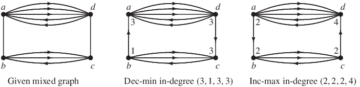
In the second variant, we are interested in the in-degree vector of the digraph obtained by orienting the originally undirected part . For this version, the counterexample mixed graph is demonstrated in Figure 2. In any strong orientations of , parallel edges in must be oriented oppositely. Therefore the contribution of the actual orientations of these four pairs of parallel undirected edges (in the order of ) is .
Therefore there are essentially two distinct strong orientations of . In the first one, the undirected edges are oriented as , while in the second one the undirected edges are oriented as . Hence the in-degree vector of the first strong orientation corresponding to the orientation of (in the order of ) is . The in-degree vector of second strong orientation corresponding to the orientation of is . The first vector is inc-max while the second vector is dec-min.

These examples give rise to the question: what is behind the phenomenon that while dec-min and inc-max coincide for strong orientations of undirected graphs, they differ for strong orientations of mixed graph? The explanation is, as we pointed out earlier, that for an M-convex set the two notions coincide and the set of in-degree vectors of strong orientations of an undirected graph is an M-convex set, while the corresponding set for a mixed graph is, in general, not an M-convex set. It is actually the intersection of two M-convex sets. An algorithm for computing a dec-min element of the intersection of two M-convex sets is described in [23].
6.3 Higher edge-connectivity
An analogous approach works in a much more general setting. We say that a digraph covers a set-function if holds for every set . The following result was proved in [14].
Theorem 6.5 ([14]).
Let be a finite-valued, non-negative crossing supermodular function with . A graph has an orientation covering if and only if
hold for every partition of , where denotes the number of edges connecting distinct parts of .
This theorem easily implies the classic orientation result of Nash-Williams [48] stating that a graph has a -edge-connected orientation precisely if is -edge-connected. Namely, by defining to be identically equal to on non-empty proper subsets of while , and observing that , we can see that both inequalities in the theorem are equivalent to . But this latter inequality follows from the -edge-connectivity of since .
Even more, call a digraph -edge-connected () (with respect to a root-node ) if whenever and whenever . (By Menger’s theorem, -edge-connectedness is equivalent to requiring that there are arc-disjoint dipaths from to every node and there are arc-disjoint dipaths from every node to .) Then Theorem 6.5 implies:
Theorem 6.6.
A graph has a -edge-connected orientation if and only if
holds for every -partite partition of .
Note that an even more general special case of Theorem 6.5 can be formulated to characterize graphs admitting in-degree constrained and -edge-connected orientations.
It is important to emphasize that however general Theorem 6.5 is, it does not say anything about strong orientations of mixed graphs. In particular, it does not imply the pretty but easily provable theorem of Boesch and Tindell [5]. The problem of finding decreasingly minimal in-degree constrained -edge-connected orientation of mixed graphs can be solved as a special case of decreasing minimization over the intersection of two M-convex sets.
The next lemma shows why the set of in-degree vectors of orientations of covering the set-function appearing in Theorem 6.5 is an M-convex set, ensuring in this way the possibility of applying the results on decreasing minimization over M-convex sets to general graph orientation problems.
Lemma 6.7.
An orientation of covers if and only if its in-degree vector is in the base-polyhedron , where is a crossing supermodular function.
Proof. Suppose first that is the in-degree vector of a digraph covering . Then for and , that is, is indeed in .
Conversely, suppose that . Since is finite-valued and non-negative, we have for and and hence, by the Orientation lemma, there is an orientation of with in-degree vector . Moreover, this digraph covers since holds for .
By Lemma 6.7, Theorem 2.1 can be applied again to the general orientation problem covering a non-negative and crossing supermodular set-function in the same way as it was applied in the special case of strong orientation above, but we formulate the result only for the special case of in-degree constrained and -edge-connected orientations.
Theorem 6.8.
Let be an undirected graph endowed with a lower bound function and an upper bound function with . A -edge-connected and in-degree constrained orientation of is decreasingly minimal if and only if there are no two nodes and for which , , , and there are arc-disjoint -dipaths.
The theorem can be extended even further to in-degree constrained and -edge-connected orientations ().
Locally -edge-connected orientations
For a subset of nodes of a digraph , we say that is locally -edge-connected in if there are arc-disjoint dipaths in from any node of to any other node of . This is equivalent to requiring (by Menger’s theorem) that holds for each subset for which neither nor is empty. Clearly, when , we are back at ordinary -edge-connectivity. Király and Lau [41] considered a closely related concept when the requirement for is that there are edge-disjoint dipaths from a specified root-node of to every other node of . Such a digraph may be called locally rooted -edge-connected in .
By relying on a base-polyhedral approach, Király and Lau [41] proved (Theorem 1.3) that there exists a polynomial algorithm for finding an orientation of which is locally rooted -edge-connected in and the orientation meets an in-degree specification on the nodes in . By using an analogous approach, we can solve the orientation problem in which, beside the in-degree specification on , the requirement is local -edge-connectivity in . To this end, define a set-function on as follows:
It is not difficult to see that is a non-negative, crossing supermodular function on . Let denote the integral base-polyhedron defined by . By relying on Lemma 6.7, one can derive the following.
Theorem 6.9.
Let be an undirected graph with a specified subset of . Let be an in-degree specification on . The set of in-degree vectors of those orientations of which are locally -edge-connected in and in-degree specified in is an M-convex set , namely, .
By this theorem, we can determine a decreasingly minimal orientation among those which are -edge-connected in and in-degree specified in . Even additional in-degree constraints can be imposed on the elements of .
Remark 6.1.
One may consider the orientation problem where, beside local -edge-connectivity in , we impose upper and lower bounds on the in-degrees of nodes outside (instead of exact values). Bernáth et al. [4] proved that the in-degree constrained version of Nash-Willams’ well-balanced orientation problem [48] is NP-complete. By using a similar method, Bernáth [3] recently proved that already the problem is NP-complete, even in the special case with .
Hypergraph orientation
Let be a hypergraph for which we assume that each hyperedge has at least 2 nodes. Orienting a hyperedge means that we designate an element of as its head-node. A hyperedge with a designated head-node is a directed hyperedge denoted by . Orienting a hypergraph means the operation of orienting each of its hyperedges. We say that a directed hyperedge enters a subset of nodes if and . A directed hypergraph is called -edge-connected if the in-degree of every non-empty proper subset of nodes is at least .
Theorem 6.10.
The set of in-degree vectors of -edge-connected and in-degree constrained orientations of a hypergraph forms an M-convex set.
Therefore we can apply the general results obtained for decreasing minimization over M-convex sets.
Acknowledgement
We are particularly grateful to an anonymous referee of the paper whose fundamental suggestions made a significant contribution to the final form of our work. This research was supported through the program “Research in Pairs” by the Mathematisches Forschungsinstitut Oberwolfach in 2019. The two weeks we could spend at Oberwolfach provided an exceptional opportunity to conduct particularly intensive research. The research was partially supported by the National Research, Development and Innovation Fund of Hungary (FK_18) – No. NKFI-128673, and by CREST, JST, Grant Number JPMJCR14D2, Japan, and JSPS KAKENHI Grant Numbers JP26280004, JP20K11697.
References
- [1] Apollonio, N., Sebő, A.: Minconvex factors of prescribed size in graphs. SIAM Journal on Discrete Mathematics 23, 1297–1310 (2009)
- [2] Bérczi, K., Frank, A.: Supermodularity in unweighted graph optimization, Part I: Branchings and matchings. Mathematics of Operations Research 43, 726–753 (2018)
- [3] Bernáth, A.: Personal communication (2021)
- [4] Bernáth, A., Iwata, S., Király, T., Király, Z, Szigeti, Z.: Recent results on well-balanced orientations. Discrete Optimization 5, 663–676 (2008)
- [5] Boesch, F., Tindell, R.: Robbins’s theorem for mixed multigraphs. American Mathematical Monthly 87, 716–719 (1980)
- [6] Bokal, D., Brešar, B., Jerebic, J.: A generalization of Hungarian method and Hall’s theorem with applications in wireless sensor networks. Discrete Applied Mathematics 160, 460–470 (2012)
- [7] Borradaile, G., Iglesias, J., Migler, T., Ochoa, A., Wilfong, G., Zhang, L.: Egalitarian graph orientations. Journal of Graph Algorithms and Applications 21, 687–708 (2017)
- [8] Borradaile, G., Migler, T., Wilfong, G.: Density decompositions of networks. Journal of Graph Algorithms and Applications 23, 625–651 (2019)
- [9] Edmonds, J.: Submodular functions, matroids and certain polyhedra. In: Guy, R., Hanani, H., Sauer, N., Schönheim, J. (eds.) Combinatorial Structures and Their Applications, pp. 69–87. Gordon and Breach, New York (1970)
- [10] Edmonds, J.: Edge-disjoint branchings. In: Rustin, B. (ed.) Combinatorial Algorithms, pp. 91–96. Academic Press, New York (1973)
- [11] Edmonds, J.: Matroid intersection. Annals of Discrete Mathematics 14, 39–49 (1979)
- [12] Federgruen, A., Groenevelt, H.: The greedy procedure for resource allocation problems: necessary and sufficient conditions for optimality. Operations Research 34, 909–918 (1986)
- [13] Ford, L. R., Jr., Fulkerson, D.R.: Flows in Networks. Princeton University Press, Princeton NJ (1962)
- [14] Frank, A.: On the orientation of graphs. Journal of Combinatorial Theory, Ser. B 28, 251–261 (1980)
- [15] Frank, A.: Augmenting graphs to meet edge-connectivity requirements. SIAM Journal on Discrete Mathematics 5, 22–53 (1992)
- [16] Frank, A.: Connections in Combinatorial Optimization. Oxford University Press, Oxford (2011)
- [17] Frank, A., Jordán, T.: Minimal edge-coverings of pairs of sets. Journal of Combinatorial Theory, Ser. B 65, 73–110 (1995)
- [18] Frank, A., Király, T.: A survey on covering supermodular functions. In: Cook, W., Lovász, L., Vygen, J. (eds.) Research Trends in Combinatorial Optimization, pp. 87–126. Springer, Berlin (2009)
- [19] Frank, A., Király, T., Király, Z.: On the orientation of graphs and hypergraphs. Discrete Applied Mathematics 131, 385–400 (2003)
- [20] Frank, A., Murota, K.: Discrete decreasing minimization, Part II: Views from discrete convex analysis. arXiv: 1808.08477 (August 2018)
- [21] Frank, A., Murota, K.: Decreasing minimization on M-convex sets: Background and structures. Submitted for publication. arXiv: 2007.09616 (July 2020)
- [22] Frank, A., Murota, K.: Fair integral flows. Submitted for publication. arXiv: 1907.02673 (September 2020)
- [23] Frank, A., Murota, K.: Fair integral submodular flows. arXiv: 2012.07325 (December 2020)
- [24] Frank, A., Tardos, É.: Generalized polymatroids and submodular flows. Mathematical Programming 42, 489–563 (1988)
- [25] Fujishige, S.: Lexicographically optimal base of a polymatroid with respect to a weight vector. Mathematics of Operations Research 5, 186–196 (1980)
- [26] Fujishige, S.: Structures of polyhedra determined by submodular functions on crossing families. Mathematical Programming 29, 125–141 (1984)
- [27] Fujishige, S.: Submodular Functions and Optimization, 2nd edn. Annals of Discrete Mathematics 58, Elsevier, Amsterdam (2005)
- [28] Goemans, M.X., Gupta, S., Jaillet, P.: Discrete Newton’s algorithm for parametric submodular function minimization. In: Eisenbrand, F., Koenemann, J. (eds.) Integer Programming and Combinatorial Optimization. Lecture Notes in Computer Science, vol. 10328, pp. 212–227 (2017)
- [29] Hakimi, S.L.: On the degrees of the vertices of a directed graph. Journal of The Franklin Institute 279, 290–308 (1965)
- [30] Harada, Y., Ono, H., Sadakane, K., Yamashita, M.: Optimal balanced semi-matchings for weighted bipartite graphs. IPSJ Digital Courier 3, 693–702 (2007)
- [31] Harvey, N.J.A., Ladner, R.E., Lovász, L., Tamir, T.: Semi-matchings for bipartite graphs and load balancing. Journal of Algorithms 59, 53–78 (2006)
- [32] Hochbaum, D.S.: Complexity and algorithms for nonlinear optimization problems. Annals of Operations Research 153, 257–296 (2007)
- [33] Hochbaum, D.S., Hong, S.-P.: About strongly polynomial time algorithms for quadratic optimization over submodular constraints. Mathematical Programming 69, 269–309 (1995)
- [34] Hoffman, A.J.: Some recent applications of the theory of linear inequalities to extremal combinatorial analysis. In: Bellman, R., Hall, M., Jr. (eds.) Combinatorial Analysis (Proceedings of the Symposia of Applied Mathematics 10) pp. 113–127. American Mathematical Society, Providence, Rhode Island (1960)
- [35] Ibaraki, T., Katoh, N.: Resource Allocation Problems: Algorithmic Approaches. MIT Press, Boston (1988)
- [36] Iwata, S., Fleischer, L., Fujishige, S.: A combinatorial, strongly polynomial-time algorithm for minimizing submodular functions. Journal of the ACM 48, 761–777 (2001)
- [37] Jiang, H.: Minimizing convex functions with integral minimizers. In: Proceedings of the 2021 ACM-SIAM Symposium on Discrete Algorithms (SODA), SIAM, pp. 976–985 (2021)
- [38] Katoh, N., Ibaraki, T.: Resource allocation problems. In: Du, D.-Z., Pardalos, P.M. (eds.) Handbook of Combinatorial Optimization, Vol.2, pp. 159–260. Kluwer Academic Publishers, Boston (1998)
- [39] Katoh, N., Shioura, A., Ibaraki, T.: Resource allocation problems. In: Pardalos, P.M., Du, D.-Z., Graham, R.L. (eds.) Handbook of Combinatorial Optimization, 2nd ed., Vol. 5, pp. 2897-2988, Springer, Berlin (2013)
- [40] Katrenič, J., Semanišin, G.: Maximum semi-matching problem in bipartite graphs. Discussiones Mathematicae, Graph Theory 33, 559–569 (2013)
- [41] Király, T., Lau, L.-C.: Approximate min-max theorems for Steiner rooted-orientations of graphs and hypergraphs. Journal of Combinatorial Theory, Ser. B 98, 1233–1252 (2008)
- [42] Levin, A., Onn, S.: Shifted matroid optimization. Operations Research Letters 44, 535–539 (2016)
- [43] Megiddo, N.: Optimal flows in networks with multiple sources and sinks. Mathematical Programming 7, 97–107 (1974)
- [44] Megiddo, N.: A good algorithm for lexicographically optimal flows in multi-terminal networks. Bulletin of the American Mathematical Society 83, 407–409 (1977)
- [45] Moriguchi, S., Shioura, A., Tsuchimura, N.: M-convex function minimization by continuous relaxation approach—Proximity theorem and algorithm. SIAM Journal on Optimization 21, 633–668 (2011)
- [46] Murota, K.: Discrete convex analysis. Mathematical Programming 83, 313–371 (1998)
- [47] Murota, K.: Discrete Convex Analysis. Society for Industrial and Applied Mathematics, Philadelphia (2003)
- [48] Nash-Williams, C.St.J.A.: On orientations, connectivity and odd vertex pairings in finite graphs. Canadian Journal of Mathematics 12, 555–567 (1960)
- [49] Orlin, J.B.: A faster strongly polynomial time algorithm for submodular function minimization. Mathematical Programming, Series A 118, 237–251 (2009)
- [50] Radzik, T.: Fractional combinatorial optimization. In: Pardalos, P.M., Du, D.-Z., Graham, R.L. (eds.) Handbook of Combinatorial Optimization, 2nd edn., pp. 1311–1355. Springer Science+Business Media, New York (2013)
- [51] Robbins, H.E.: A theorem on graphs with an application to a problem of traffic control. American Mathematical Monthly 46, 281–283 (1939)
- [52] Schrijver, A.: A combinatorial algorithm minimizing submodular functions in strongly polynomial time. Journal of Combinatorial Theory, Series B 80, 346–355 (2000)
- [53] Schrijver, A.: Combinatorial Optimization: Polyhedra and Efficiency. Springer, Heidelberg (2003)
- [54] Tardos, É.: A strongly polynomial minimum cost circulation algorithm. Combinatorica 5, 247–255 (1985)
- [55] Topkis, D.M.: Minimizing a submodular function on a lattice. Operations Research 26, 305–321 (1978)
- [56] Zhou, H., Hou, X.: Strongly connected orientation with minimum lexicographic order of indegrees. arXiv:2103.01017 (March 2021)