Learning to Play Cup-and-Ball with Noisy Camera Observations
Abstract
Playing the cup-and-ball game is an intriguing task for robotics research since it abstracts important problem characteristics including system nonlinearity, contact forces and precise positioning as terminal goal. In this paper, we present a learning model based control strategy for the cup-and-ball game, where a Universal Robots UR5e manipulator arm learns to catch a ball in one of the cups on a Kendama. Our control problem is divided into two sub-tasks, namely swinging the ball up in a constrained motion, and catching the free-falling ball. The swing-up trajectory is computed offline, and applied in open-loop to the arm. Subsequently, a convex optimization problem is solved online during the ball’s free-fall to control the manipulator and catch the ball. The controller utilizes noisy position feedback of the ball from an Intel RealSense D435 depth camera. We propose a novel iterative framework, where data is used to learn the support of the camera noise distribution iteratively in order to update the control policy. The probability of a catch with a fixed policy is computed empirically with a user specified number of roll-outs. Our design guarantees that probability of the catch increases in the limit, as the learned support nears the true support of the camera noise distribution. High-fidelity Mujoco simulations and preliminary experimental results support our theoretical analysis (video link – GitHub link).
I Introduction
Kendama is the Japanese version of the classic cup-and-ball game, which consists of a handle, a pair of cups, and a ball, which are all connected by a string. Playing the cup-and-ball game is a task commonly considered in robotics research [1, 2, 3, 4, 5, 6, 7, 8], where approaches ranging from classical PD control to reinforcement learning have been utilized to solve the task. The model-based approaches among the above typically decompose the task into two sub-tasks, namely performing a swing-up of the ball when the string is taut, and catching the ball during its free-fall. The models of the joint system considered for both sub-tasks are different, thus resulting in hybrid control design for the robotic manipulator. The key drawbacks in such existing approaches are namely the need for expert demonstrations, and the lack of guarantees of operating constraint satisfaction and obtaining catches under modeling uncertainty and sensing errors.
In this paper, we propose a fully physics driven model-based hybrid approach for control design. The controller guarantees a constrained motion, while accounting for our best estimates of uncertainty in the system model and sensing errors. We use a mixed open-loop and closed-loop control design, motivated by works such as [9, 10, 11]. First, the swing-up phase is designed offline and then an open-loop policy is applied to the robotic manipulator. We use a cart with inverted pendulum model of the cup-and-ball joint system for swing-up policy design. For this phase, as we solve a constrained finite horizon non-convex optimization problem, we only consider a nominal disturbance-free model of the system. The swing-up trajectory is thus designed to ensure that the predicted difference in positions of the ball and the cup vanishes at a future time once the nominal terminal swing-up state is reached and the cup is held fixed.
After a swing-up, we switch to online closed-loop control synthesis once the ball starts its free-fall. We consider presence of only a camera that takes noisy measurements of the ball’s position at every time step. We design the feedback controller in the manipulator’s end-effector [12] space. This results in a Linear Time Invariant (LTI) model for the evolution of the difference between the cup and the ball’s positions, thus allowing us to solve convex optimization problems online for control synthesis. In order to guarantee a catch by minimizing the position difference, it is also crucial to ensure that during the free-fall of the ball, the control actions to the manipulator do not yield a configuration where the string is taut, despite uncertainty in the model and noise in camera position measurements. Uncertainty in the LTI model primarily arises from low level controller mismatches in the manipulator hardware, and an upper bound of this uncertainty is assumed known. Bounds on the measurement noise induced by the camera are assumed unknown. This paper presents a method to increase the probability of a catch, as the estimate of the support of camera measurement noise distribution is updated. Our contributions are summarized as:
- •
Offline, before the feedback control of the manipulator, we design a swing-up trajectory for the nominal cup-and-ball system that plans the motion of the ball to a state from which a catch control is initiated.
- •
Using the notion of Confidence Support from [13] which is guaranteed to contain the true support of the camera measurement noise with a specified probability, we use online robust feedback control for enforcing bounds on the probability of failed catches.
- •
With high-fidelity Mujoco simulations and preliminary physical experiments we demonstrate that the manipulator gets better at catching the ball as the support of the camera measurement noise is learned and as the Confidence Support and closed-loop policy are updated.
II Generating A Swing-up Trajectory
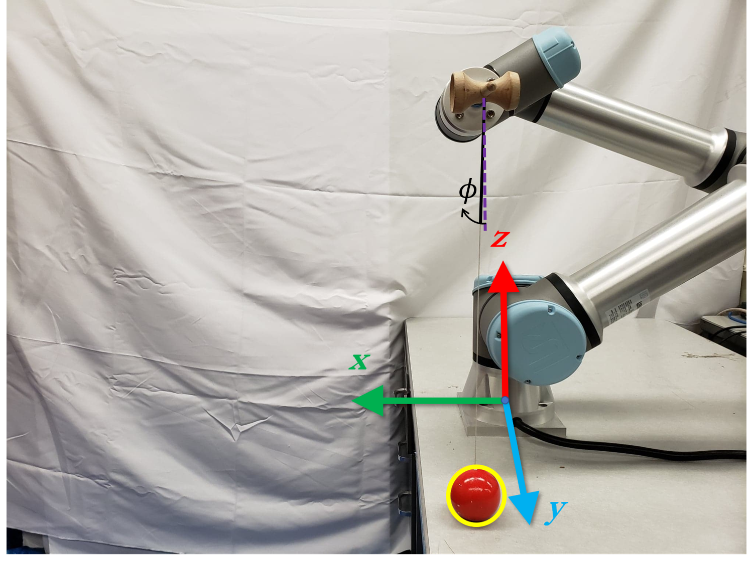
The swing-up phase begins with the arm in the home position such that the ball is hanging down at an angle of radians from the vertical plumb line, as seen in Fig. 1.
II-A System Modeling
We model the system such that the cup is a planar cart with point-mass and the ball acts as a rigid pendulum (mass and radius ) attached to the cup. Assuming planar -motion of the ball, we derive the Lagrange equations of motion [12] with three generalized coordinates , which denote the position of the cup, position of the cup, and swing angle of the ball with respect to the plumb line of the cup respectively at any time . We reduce the equations to the general nominal form
| (1) |
where is the inertia matrix, is the Coriolis matrix, is the gravity matrix, and is the external input force at time . Here denotes the velocity of the cup and the angular velocity of the ball, and denotes the acceleration of the cup and the angular acceleration of the ball at any time . System (1) in state-space form is
| (2) |
where nominal state for all time .
II-B Optimization Problem
We discretize system (2) with one step Euler discretization and a sampling time of Hz. The discrete time system can then be written as
where denotes the sampled time version of continuous variable . To generate a force input sequence for the swing-up, we solve a constrained optimal control problem over a finite planning horizon of length , given by:
| (3) |
where weight matrices , and constraint set is chosen such that the ball remains within the reach of the UR5e manipulator. Initial state is known in the configuration as shown in Fig. 1. Due to the nonlinear dynamics , the optimization problem (3) is non-convex. Moreover, typically a long horizon length is required. Hence, we solve (3) offline and apply the computed input sequence in open-loop to the manipulator.
II-C Terminal Conditions of the Swing-Up
Predicted Behaviour
The nominal terminal state in (3) is selected such that the ball is swinging to rad with an angular velocity of rad/s. At these values, the string is calculated to lose tension and the ball begins free-fall. The chosen value of ensures that the predicted difference in positions of the ball and the cup (both modeled as point masses) vanishes at a future time, if the cup were held fixed and the ball’s motion is predicted under free-fall.
Actual Behaviour
When considering the nominal system (1), we have ignored the presence of uncertainties. Such uncertainties may arise due to our simplifying assumptions such as: the string is mass-less so the swing angle is only affected by the ball and cup masses, there are no frictional and aerodynamic drag forces to hinder the conservation of kinetic and potential energy of the system, the cup mass is decoupled from the mass of the manipulator, and there is no mismatch of control commands from the low level controller of the manipulator and . Due to such uncertainties, realized states for do not exactly match their nominal counterparts.
A set of 100 measured roll-out trajectories of the ball after the swing-up are shown in Fig. 2 for a fixed open-loop input sequence .
We see from Fig. 2 that after time steps of swing-up, the ball and the cup arrive at positions where their relative position is in a set . A key assumption of well posedness will be imposed on this set in Section III-D in order for our subsequent feedback control policy to deliver a catch in experiments.
III Designing Feedback Policy In Catch Phase
For the catch phase we start the time index where the swing up ends, i.e., . There are two main challenges during the design of the feedback controller, namely position measurements of the ball from a noisy camera, and presence of mismatch between desired control actions and corresponding low level controller commands.
Assumption 1
We assume that the UR5e end-effector gives an accurate estimate of its own position. The assumption is based on precision ranges provided in [14].
III-A Problem Formulation
During free-fall of the ball we design our feedback controller for the manipulator position only in end-effector space, with desired velocity of the end-effector as our control input. The joint ball and end-effector system in one trial can be modeled as a single integrator as:
| (4a) | ||||
| (4b) | ||||
with error states and inputs (i.e., relative position and velocity)
where , is a bounded uncertainty which arises due to the discrepancy between the predicted and the actual velocity of the ball at any given time step11 1 we use the camera position information for ball’s velocity estimation, and the commanded and the realized velocities of the end-effector, primarily due to the low level controller delays and limitations. System dynamics matrices and are known, where denotes the identity matrix of size , and sampling time second. We assume an outer approximation to the set , i.e., is known, and is a polytope. We consider noisy measurements of states due to the noise in camera position measurements, corrupted by , with , where denotes the support of a distribution. We assume is not exactly known.
Using the set (see Fig. 2), a set containing the origin where the string is not taut and (4) is valid can then be chosen. We choose:
| (5) |
where denotes row of all the vertices of the polytope , and denotes the vector norm. This ensures
| (6) |
As (6) holds true, we impose state and input constraints for all time steps as given by:
| (7) |
where set is a polytope. We formulate the following finite horizon robust optimal control problem for feedback control design:
| (8) |
where , and denote the realized system state, control input and model uncertainty at time step respectively, and denote the nominal state and corresponding nominal input. Notice that (8) minimizes the nominal cost over a task duration of length decided by the user, having considered the safety restrictions during an experiment. The cost comprises of the positive definite stage cost , and the terminal cost . We point out that, as system (4) is uncertain, the optimal control problem (8) consists of finding , where are state feedback policies.
The main challenge in solving problem (8) is that it is difficult to obtain the camera measurement noise distribution support . Resorting to worst-case a-priori set estimates of as in [15, 16] might result in loss of feasibility of (8). To avoid this, we use a data-driven estimate of denoted by , where is the number of samples of noise used to construct the set.
III-B Control Formulation
As we have noisy output feedback in (12), we follow [17] for a tractable constrained finite time optimal controller design strategy. We repeatedly solve (8) at times in a shrinking horizon fashion [18, Chapter 9]. We make the following assumption for this purpose:
Assumption 2
The sets , and contain the origin in their interior.
III-B1 Observer Design and Control Policy Parametrization
We design a Luenberger observer for the state as
where the observer gain is chosen such that is Schur stable. The control policy parametrization for solving (8) is chosen as:
where state feedback policy gain matrix is chosen such that is Schur stable.
III-B2 Optimal Control Problem
Consider the tightened constraint sets,
| (9a) | ||||
| (9b) | ||||
where following [17, Proposition 1-2], the set is our best estimate of the minimal Robust Positive Invariant set for the estimation error dynamics defined as
| (10) |
and the set is our best estimate of the minimal Robust Positive Invariant set for the control error dynamics defined as
| (11) |
with and . We use the phrase best estimate for the above sets, since is an estimate of true and unknown set .
Using these sets we then solve the following tractable finite horizon constrained optimal control problem at any time step as an approximation to (8):
| (12) | ||||
where is the observed state at time step , and denote the nominal state and corresponding input respectively predicted at time step . After solving (12), in closed-loop we apply
| (13) |
to system (4). We then resolve the problem (12) again at the next -th time step, yielding a shrinking horizon strategy. The choice of initial observer state is made as follows:
| (14) |
Assumption 3 (Manipulator Speed)
If any feasible solution is found to (12) satisfying velocity error constraints , the manipulator has enough velocity authority to satisfy these constraints, where the predicted ball velocity is obtained using forward Euler integration at free-fall.
Recall the set containing the set of all possible errors at the start of the catch phase, shown in Fig. 2. We now make the following assumption.
Assumption 4 (Well Posedness)
Definition 1 (Trial Failure)
Note that a Trial Failure is a possible scenario only because is unknown and is estimated with in (12). Intuitively, a Trial Failure implies one of the following:
III-C Constructing Set
As described in Section III-A the set is an estimate of the measurement noise support , derived from samples of noise . The set is then used to compute and in (10)-(11), used in (12) and (14). We consider the following two design specifications while constructing set , given a fixed sample size .
- (D1)
Probability of the event is bounded with a user specified upper bound .
- (D2)
Estimate ensures event (P2) in Trial Failure occurs with a vanishing probability, while satisfying specification (D1).
Satisfying (D1) using Distribution Information
Fig. 1 shows the configuration of the system when noise samples are collected to construct . Let Assumption 1 hold true and the ball is held still, vertically below the end-effector at a position, whose -coordinate is fixed and known from previous UR5e end-effector measurements, and -coordinate is fixed at . We then collect camera position measurements of the ball at this configuration. The discrepancy between the known position and the measurements yield values of noise samples . For a fixed environment,22 2 camera environment is parametrized by say lighting conditions, camera field of view, etc. the distribution of collected samples is shown in Fig. 3, which is approximately a truncated normal distribution.
We thereby consider this distribution family in Fig. 3 conditioned on any environment as
| (15) |
where denotes that the distribution belongs to a parametric family (truncated normal) parametrized by , denotes the dimension ( and directions), and parameters are unknown. For a parametric distribution such as (15), for any chosen , set is then constructed as the -Confidence Support of using the method in [13], which ensures
| (16) |
Note that (16) is a sufficient condition to guarantee that if (D2) holds, solving (12) and applying (13) to (4) gives
| (17) |
if is used to construct sets and .
Satisfying (D2) using Assumption 4
Since Assumption 4 holds, there exists a number of noise samples for any , such that satisfies (D2). Thus, only the sample size has to be chosen33 3 for fixed, can be increased while constructing to satisfy (D2). for appropriately to satisfy (D2), having ensured (17). This guarantees that constructing sets and using and then designing a feedback control by solving (12) results in problem (12) being feasible throughout the task with probability at least . Value of can be chosen small enough for any user-specified level can be attained.
III-D Obtaining Catches
Constructing as per Section III-C to ensure (17) is still not a sufficient condition to obtain a catch in an experiment with specified probability , as our model (4) does not account for additional factors such as object dimensions, presence of contact forces, etc.
To that regard, we introduce the notion of a successful catch, which is defined as the ball successfully ending up inside the cup at the end of a roll-out. Thus, a successful catch accounts for the dimensions of the ball and the cup, and the presence of contact forces.
Assumption 5 (Existence of a Successful Catch)
We assume that given an initial state , an input policy obtained by solving (12) can yield a successful catch, if true measurement noise support were known exactly.
Remark 1
From [13] we know that as long as confidence intervals for parameters in (15) converge, as . So, if sample size is increased iteratively approaching , obtaining a successful catch guaranteed owing to Assumption 5. However if a precise positioning system like Vicon is used to collect the noise samples, due to limited access to such environments, collecting more samples and increasing could be expensive. We therefore stick to our method of constructing for a fixed as per Section III-C, and we attempt successful catches with multiple roll-outs by solving (12). For improving the empirical probability of successful catches in these roll-outs, one may then increase and thus update the control policy. We demonstrate this in Section IV-B.
IV Experimental Results
We present our preliminary experimental findings in this section. For our experiments, the original Kendama handle was modified to be attached to a 3D printed mount on the UR5e end-effector, as shown in Fig. 1. A single Intel RealSense D435 depth camera running at 60 FPS was used to estimate the position and velocity of the ball.
IV-A Control Design in the Catch Phase
Once the swing-up controller is designed as per Section II-B and an open-loop swing-up control sequence is applied to the manipulator, we design the feedback controller by finding approximate solutions to the following problem:
| (18) |
where set , shown in Fig. 2. Note that for this specific scenario the presence of model uncertainty can be ignored. Set is unknown, and we consider Assumption 4 holds. System matrices are from Section III-A. We find solutions to (18) for , i.e., seconds.
IV-B Learning to Catch
We conduct roll-outs of the catching task by solving (12), having formed as per Section III-C, with and then iteratively increasing to . Sets are formed using [13]. Fig. 4 shows the percentage of roll-outs conducted for each iteration (i.e., for each value of ), that resulted in the ball successfully striking the center of the cup.
The percentage increases from to . Furthermore, another crucial quantity at the time of impact is the commanded relative velocity (13) in -direction, a lower value of which indicates an increased likelihood of the ball not bouncing out. The average value and the standard deviation of of for is shown in Fig. 5, where denotes the roll-out and denotes the time of impact.
IV-C Increasing Successful Catches
In order to prove that the trend shown in Fig. 4 and Fig. 5 results in an increasing number of successful catches, we resort to exhaustive Mujoco [19, 20] simulations44 4 due to unavailability of laboratory access. The task duration in this case is .
The trend in the percentage of successful catches with 1000 roll-outs corresponding to each , varying from to , is shown in Fig. 6. For , of the roll-outs result in a successful catch. The number increases to for . This verifies that the preliminary experimental results from Fig. 4 and Fig. 5 would very likely result in a similar trend as in Fig. 6. Thus we prove that our proposed approach enables successful learning of the kendama ball catching task.
V Conclusions
We proposed a model based control strategy for the classic cup-and-ball game. The controller utilized noisy position measurements of the ball from a camera, and the support of this noise distribution was iteratively learned from data. Thus, the closed-loop control policy iteratively updates. We proved that the probability of a catch increases in the limit, as the learned support nears the true support of the camera noise distribution. Preliminary experimental results and high-fidelity simulations support our analysis.
Acknowledgement
We thank Yuri Glauthier, Charlott Vallon, and Sangli Teng for their contributions on the hardware experiments, as well as Vijay Govindarajan, Siddharth Nair and Edward Zhu for extremely useful reviews and discussions. The research was funded by grants ONR-N00014-18-1-2833, NSF-1931853, and Siemens.
References
- [1] B. Nemec and A. Ude, “Reinforcement learning of ball-in-a-cup playing robot,” in 2011 IEEE International Conference on Robotics and Biomimetics, Dec 2011, pp. 2682–2987.
- [2] J. Kober and J. Peters, “Learning motor primitives for robotics,” in 2009 IEEE International Conference on Robotics and Automation, May 2009, pp. 2112–2118.
- [3] H. Miyamoto, S. Schaal, F. Gandolfo, H. Gomi, Y. Koike, R. Osu, E. Nakano, Y. Wada, and M. Kawato, “A kendama learning robot based on bi-directional theory,” Neural Networks, vol. 9, no. 8, pp. 1281 – 1302, 1996.
- [4] T. Sakaguchi and F. Miyazaki, “Dynamic manipulation of ball-in-cup game,” in Proceedings of the 1994 IEEE International Conference on Robotics and Automation, May 1994, pp. 2941–2948 vol.4.
- [5] A. Namiki and N. Itoi, “Ball catching in kendama game by estimating grasp conditions based on a high-speed vision system and tactile sensors,” in 2014 IEEE-RAS International Conference on Humanoid Robots, Nov 2014, pp. 634–639.
- [6] D. Schwab, T. Springenberg, M. F. Martins, T. Lampe, M. Neunert, A. Abdolmaleki, T. Herkweck, R. Hafner, F. Nori, and M. Riedmiller, “Simultaneously learning vision and feature-based control policies for real-world ball-in-a-cup,” arXiv preprint arXiv:1902.04706, 2019.
- [7] T. Senoo, A. Namiki, and M. Ishikawa, “Ball control in high-speed batting motion using hybrid trajectory generator,” in Proceedings 2006 IEEE International Conference on Robotics and Automation, 2006. ICRA 2006., May 2006, pp. 1762–1767.
- [8] S. Li, “Robot playing kendama with model-based and model-free reinforcement learning,” arXiv preprint arXiv:2003.06751, 2020.
- [9] E. A. Hansen, A. G. Barto, and S. Zilberstein, “Reinforcement learning for mixed open-loop and closed-loop control,” in NIPS, 1996.
- [10] C. G. Atkeson and S. Schaal, “Learning tasks from a single demonstration,” in Proceedings of International Conference on Robotics and Automation, vol. 2, 1997, pp. 1706–1712.
- [11] J. Z. Kolter, C. Plagemann, D. T. Jackson, A. Y. Ng, and S. Thrun, “A probabilistic approach to mixed open-loop and closed-loop control, with application to extreme autonomous driving,” in 2010 IEEE International Conference on Robotics and Automation, 2010, pp. 839–845.
- [12] R. M. Murray, Z. Li, and S. S. Sastry, A mathematical introduction to robotic manipulation. CRC press, 1994.
- [13] M. Bujarbaruah, A. Shetty, K. Poolla, and F. Borrelli, “Learning robustness with bounded failure: An iterative MPC approach,” arXiv preprint arXiv:1911.09910, 2019.
- [14] U. Robots, “e-Series from universal robots,” https://www.universal-robots.com/media/1802432/e-series-brochure.pdf, 2014.
- [15] M. Tanaskovic, L. Fagiano, R. Smith, and M. Morari, “Adaptive receding horizon control for constrained mimo systems,” Automatica, vol. 50, no. 12, pp. 3019–3029, 2014.
- [16] X. Lu and M. Cannon, “Robust adaptive tube model predictive control,” in 2019 IEEE American Control Conference (ACC). IEEE, Jul. 2019, pp. 3695–3701.
- [17] D. Q. Mayne, S. Raković, R. Findeisen, and F. Allgöwer, “Robust output feedback model predictive control of constrained linear systems,” Automatica, vol. 42, no. 7, pp. 1217–1222, 2006.
- [18] F. Borrelli, A. Bemporad, and M. Morari, Predictive control for linear and hybrid systems. Cambridge University Press, 2017.
- [19] E. Todorov, T. Erez, and Y. Tassa, “Mujoco: A physics engine for model-based control,” in 2012 IEEE/RSJ International Conference on Intelligent Robots and Systems. IEEE, 2012, pp. 5026–5033.
- [20] Y. Tassa, S. Tunyasuvunakool, A. Muldal, Y. Doron, S. Liu, S. Bohez, J. Merel, T. Erez, T. Lillicrap, and N. Heess, “dm_control: Software and tasks for continuous control,” arXiv preprint arXiv:2006.12983, 2020.