Gaussian Kernel Smoothing

Kernel smoothing is the most widely used image smoothing technique in brain image analysis. Consider the integral transform

$\displaystyle Y(t)=\int K(t,s)X(s)\;ds,$

where $K$ is the kernel of the integral. Given the input signal $X$, $Y$ represents the output signal. The smoothness of the output depends on the smoothness of the kernel. We assume the kernel to be unimodal and isotropic. When the kernel is isotropic, it has radial symmetry and should be invariant under rotation. So it has the form

$$K(t,s)=f(\|t-s\|)$$

for some smooth function $f$. Since the kernel only depends on the difference of the arguments, with the abuse of notation, we can simply write $K$ as

$$K(t,s)=K(t-s).$$

We may further assume the kernel is normalized such that

$$\int K(t)\;dt=1.$$

With this specific form of kernel $K$, (1) can be written as

$\displaystyle Y(t)=K*X(t)=\int K(t-s)X(s)\;ds.$

The integral transform (1) is called kernel smoothing. We may assume further that $K$ is dependent on bandwidth $\sigma$. The bandwidth will determine the spread of kernel weights such that

	$\displaystyle\lim_{\sigma\to\infty}K(t,s;\sigma)$	$\displaystyle=$	$\displaystyle 1$		(1)
	$\displaystyle\lim_{\sigma\to 0}K(t,s;\sigma)$	$\displaystyle=$	$\displaystyle\delta(t-s),$		(2)

where $\delta$ is the Dirac-delta function (Berline et al. 1991; Dirac 1981). The Dirac-delta function is a special case of generalized functions (Gelfand et al. 1964; Stakgold 2000). The Dirac-delta function is usually traditionally defined as

$$\delta(t)=0\mbox{ if }t\neq 0,\quad\delta(t)=\infty\mbox{ if }t=0.$$

$$\int_{-\infty}^{\infty}\delta(t)\;dt=1.$$

The Dirac delta function is also referred to as the impulse function in literature. Figure 1 illustrates 1D Gaussian kernel smoothing in simulated data. One of the important properties of Dirac delta function is

$$\int_{-\infty}^{\infty}f(t)\delta(t)\;dt=f(0).$$

Then it follows the one of most important operational characteristic of Dirac delta:

$\displaystyle K*\delta(t)=\int_{-\infty}^{\infty}K(t-s)\delta(s)\;ds=K(t).$

(3)

All brain images are inherently noisy due to errors associated with image acquisition. Compounding the image acquisition errors, there are errors caused by image registration and segmentation. So it is necessary to smooth out the segmented images before any statistical analysis is performed to boost statistical power. Among many possible kernel smoothing methods (Kovačič & Bajcsy 1999; Perona & Malik 1990), Gaussian kernel smoothing has emerged as a de facto smoothing technique in brain imaging.

The Gaussian kernel in 1D is defined as

$$K(t)=\frac{1}{\sqrt{2\pi}}e^{t^{2}/2}.$$

Let’s scale the Gaussian kernel $K$ by the bandwidth $\sigma$:

$$K_{\sigma}(t)=\frac{1}{\sigma}K\Big(\frac{t}{\sigma}\Big).$$

This is the density function of the normal distribution with mean $0$ and variance $\sigma^{2}$.

The $n$-dimensional isotropic Gaussian kernel is defined as the product of $n$ 1D kernels. Let $t=(t_{1},\cdots,t_{n})^{\top}\in\mathbb{R}^{n}.$ Then the $n$-dimensional kernel is given by

	$\displaystyle K_{\sigma}(t)$	$\displaystyle=$	$\displaystyle K_{\sigma}(t_{1})K_{\sigma}(t_{2})\cdots K_{\sigma}(t_{n})$
		$\displaystyle=$	$\displaystyle\frac{1}{(2\pi)^{n/2}\sigma^{n}}\exp\Big(\frac{1}{2\sigma^{2}}\sum_{i=1}^{n}t_{i}^{2}\Big).$

Subsequently, $n$-dimensional isotropic Gaussian kernel smoothing $K_{\sigma}*X$ can be done by applying 1-dimensional smoothing $n$ times in each direction by factorizing the kernel as

	$\displaystyle K_{\sigma}*X(t)$	$\displaystyle=$	$\displaystyle\int K_{\sigma}(t-s)X(s)\;ds$
		$\displaystyle=$	$\displaystyle\int K_{\sigma}(t_{1}-s_{1})K_{\sigma}(t_{2}-s_{2})\cdots K_{\sigma}(t_{n}-s_{n})X(s)\;ds$
		$\displaystyle=$	$\displaystyle\int K_{\sigma}(t_{1}-s_{1})\cdots K_{\sigma}(t_{n-1}-s_{n-1})\;ds_{1}\cdots ds_{n-1}$
			$\displaystyle\times\int K_{\sigma}(t_{n}-s_{n})X(s)\;ds_{n}.$

Note that $K_{\sigma}*X$ is the scale-space representation of image $X$ first introduced in (Witkin 1983). Each $K_{\sigma}*X$ for different values of $\sigma$ produces a blurred copy of its original. The resulting scale-space representation from coarse to fine resolution can be used in multiscale approaches such as hierarchical searches and image segmentation (Lindeberg 1994; Poline & Mazoyer 1994; Poline et al. 1995; Worsley, Marrett, Neelin, Vandal, Friston & Evans 1996; Worsley, Marrett, Neelin & Evans 1996).

The bandwidth $\sigma$ defines the spread of kernel. In brain imaging, the spread of the kernel is usually measured in terms of the full width at the half maximum (FWHM) of Gaussian kernel $K_{\sigma}$, which is given by $2\sqrt{2\ln 2}\sigma$. This can be easily seen by representing the kernel using the radius $r^{2}=x_{1}^{2}+\cdots x_{n}^{2}$:

$$K_{\sigma}(r)=\frac{1}{(2\pi)^{n/2}\sigma^{n}}\exp\Big(-\frac{r^{2}}{2\sigma^{2}}\Big).$$

The peak of the kernel is $K_{\sigma}(0)$. Then the full width at half maximum (FWHM) of the peak is given by

$$\mbox{ FWHM}=2\sqrt{2\ln 2}\sigma.$$

The FWHM increases linearly as $\sigma$ increases in Euclidean space.

Once we smooth the image with kernel $K_{\sigma}$, the smoothness of the image changes. The smoothness of image after smoothing can be measured in terms of effective FWHM. The unbiased estimator of eFWHM is first introduced in (Worsley et al. 1999), where it is estimated along edges in the lattice. Label the two voxels at the end of an edge by 1 and 2. Let the length of edge be $\Delta x$. Suppose there are $n$ images in a group. Let $r_{ij}$ denote the residual for the $i$-th image at voxel $j$. The normalized residuals at the two ends are

$$u_{ij}=\frac{r_{ij}}{\sqrt{\sum_{i=1}^{n}r_{ij}^{2}}}.$$

The roughness of the noise is defined as the standard deviation of the derivative of the noise divided by the standard deviation of the noise itself. Let

$$\Delta u=\sqrt{\sum_{i=1}^{n}(u_{i1}-u_{i2})^{2}}.$$

Then an unbiased estimator of the roughness is given by

$$\lambda=\frac{\Delta u}{\Delta x}.$$

Then the eFWHM along the edge is given by

$$e\mbox{FWHM}=\frac{\sqrt{4ln2}}{\lambda}.$$

The effective-FWHM is often used in the random field theory based on multiple comparisons correction through the fMRISTAT package (Worsley et al. 2004).

We present 1D and 2D Gaussian kernel smoothing here as illustrations using MATLAB. The codes and relevant image examples can be downloaded from http://brainimaging.waisman.wisc.edu/~chung/BIA/download/matlab.v1. The corresponding Matlab script is chapter04-smoothing.m.

K=inline(’exp(-(x.^2)/2/sigma^2)’);
dx= -5:5;

sum(K(10,dx))
weight=K(10,dx)/sum(K(10,dx))
sum(weight)

t=1:100;
mu=(t-50).^2/500;
noise= normrnd(0, 2, 1,100);
Y=mu + noise
figure; plot(Y, ’.’);

smooth=conv(Y,weight,’same’);
hold on; plot(smooth, ’r’);

[px,py] = meshgrid([0:0.01:1]);

>>px(1:3,1:3)

ans =
         0    0.0100    0.0200
         0    0.0100    0.0200
         0    0.0100    0.0200
         ...

>>py(1:3,1:3)

ans =
         0         0         0
    0.0100    0.0100    0.0100
    0.0200    0.0200    0.0200
    ...

mu=cos(10*px)+sin(8*py);
e=normrnd(0,0.4,101,101);
Y=mu+e;
figure; imagesc(Y); colorbar;

>>K=inline(’exp(-(x.^2+y.^2)/2/sig^2)’)

K =
     Inline function:
     K(sig,x,y) = exp(-(x.^2+y.^2)/2/sig^2)

[dx,dy]=meshgrid([-2:2]);
>>weight=K(0.5,dx,dy)/sum(sum(K(0.5,dx,dy)))

weight =
0.0000 0.0000 0.0002 0.0000 0.0000
0.0000 0.0113 0.0837 0.0113 0.0000
0.0002 0.0837 0.6187 0.0837 0.0002
0.0000 0.0113 0.0837 0.0113 0.0000
0.0000 0.0000 0.0002 0.0000 0.0000

>>weight=K(1,dx,dy)/sum(sum(K(1,dx,dy)))

weight =
0.0030 0.0133 0.0219 0.0133 0.0030
0.0133 0.0596 0.0983 0.0596 0.0133
0.0219 0.0983 0.1621 0.0983 0.0219
0.0133 0.0596 0.0983 0.0596 0.0133
0.0030 0.0133 0.0219 0.0133 0.0030

Ysmooth=conv2(Y,weight,’same’);
figure; imagesc(Ysmooth); colorbar;

One slice of sample T1 MRI is stored as bitmap image format as DWI.bmp, which can be read using the built-in MATLAB function imread. Stroke lesions in DWI are segmented by a human expert and stored as
DWI-segmentation.bmp.

DWimg= ’DWI’;
DWI=imread(DWimg,’bmp’);

segmentation = ’DWI-segmentation’;
f=imread(segmentation,’bmp’);

Once we read the image files, we are interested in smoothing the binary segmentation using the Gaussian kernel smoothing procedure. Bitmap files consist of a matrix of three columns representing red, green and blue colors. So we simply take out the first column and normalize it to have pixel values 0 or 1. The normalized segmentation is then smoothed using Gaussian kernel smoothing, which is implemented as tt gaussblur2D.m. The first argument to function gaussblur2D is the 2D array to smooth out and the second argument is the bandwidth given in terms of full width at the half maximum (FWHM) of the kernel.

binarize = double(f(:,:,1)/255);
fblur= gaussblur2D(binarize,10);

n=size(fblur);
fblurout = zeros(n(1), n(2), 3);
fblurout(:,:,1)=fblur;
fblurout(:,:,3)=fblur;

For visualization, we use subplot consisting of $3\times 3$ image grid. Four different images are displayed by partitioning the $3\times 3$ image grid. We have superimposed the smoothed segmentation on top of MRI by specifying the transparency of each pixel using set command with ’AlphaData’ option. Figure 3 is obtained by running the codes below.

figure; subplot(3,3,1);
imagesc(DWI);
axis off
title(’DWI’)

subplot(3,3,4);
imagesc(f);
axis off
title(’Segmentation’)

subplot(3,3,7); imagesc(fblurout)
axis off
title(’Smoothed segmentation’)

subplot(3,3,[2:3, 8:9]);
imagesc(DWI);
axis off
hold on

imgAlpha = repmat(0:1/n(2):1-1/n(2),n(1),1);
img = imagesc(fblurout);
set(img,’AlphaData’,imgAlpha);
title(’Smoothed Segmentation superimposed on DWI’)

In this section, we will explain various methods for checking Gaussianness of imaging measurements. Since many statistical models assume normality, checking if imaging data follows normality is fairly important. Also image smoothing not only increases the smoothness of underlying image intensity values, but it also increases the normality of data. In paper submissions to various imaging journals, this is an often asked question by reviewers.

p=[1:99]/100;
q=inline(’-log(1-p)/2’);
plot(q(p),p);
xlabel(’x’)
ylabel(’P(X < q)

X=exprnd(2, 500,1);
Y=exprnd(2, 500,1);
subplot(2,2,2); qqplot(X,Y)
title(’QQ-plot’)

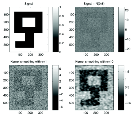
Gaussian kernel smoothing can increase the Gaussianness of multiple images. As an example, consider a key shaped binary image toy-key.tif (Figure 5). Gaussian noise with large variance is added to the binary image to mask the signal.

signal= imread(’toy-key.tif’);
signal=(double(signal)-219)/36;
figure; subplot(2,2,1); imagesc(signal); colormap(’bone’); colorbar
title(’Signal’)

noise= normrnd(0, 5, 596, 368);
f = signal + noise;
subplot(2,2,2); imagesc(f); colormap(’bone’); colorbar
title(’Signal + N(0,5)’)

To recover the signal, we performed Gaussian kernel smoothing with the bandwidths 1 and 10. For a sufficiently large bandwidth of 10, we are able to recover the underlying key shaped object. If properly used, Gaussian kernel smoothing can recover the underlying signal pretty well.

K=inline(’exp(-(x.^2+y.^2)/2/sigma^2)’);
[dx,dy]=meshgrid([-10:10]);

sigma=100;
weight=K(sigma,dx,dy)/sum(sum(K(sigma,dx,dy)));

weight=K(1,dx,dy)/sum(sum(K(1,dx,dy)));
smooth=conv2(f,weight,’same’);
subplot(2,2,3); imagesc(smooth); colormap(’bone’); colorbar
title(’Kernel smoothing with \sigma=1’)

weight=K(10,dx,dy)/sum(sum(K(10,dx,dy)));
smooth=conv2(f,weight,’same’);
subplot(2,2,4); imagesc(smooth); colormap(’bone’); colorbar
title(’Kernel smoothing with \sigma=10’)

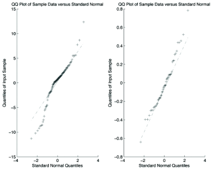
To show kernel smoothing can increase Gaussianness, we selected a pixel at $(314,150)$ which is at the edge of the binary object. For 50 measurements at the pixel, we plotted the QQ-plot. As shown in the left in Figure 6, the pixel values are not showing Gaussianness. However, after smoothing with bandwidth 100, the Gaussianness has been increased.

for i=1:50
    noise= normrnd(0, 5, 596, 368);
    weight=K(100,dx,dy)/sum(sum(K(100,dx,dy)));
    f=signal+noise;
    smooth=conv2(f,weight,’same’);
    pixelvalue(i)=f(314, 150);
    pixelvalues(i)=smooth(314, 150);
end;

figure; subplot(1,2,1); qqplot(pixelvalue)
subplot(1,2,2); qqplot(pixelvalues)

Given scatter points $x_{1},\cdots,x_{n}\in\mathbb{R}^{d}$ as observation, their empirical distribution is given by

$$f(x)=\frac{1}{n}\sum_{i=1}^{n}\delta(x-x_{i}).$$

We have impulse functions at scatter points such that

$$\int_{\mathbb{R}^{d}}f(x)\;dx=1.$$

Thus, $f$ is a probability density that is somewhere between continuous and discrete. The Dirac delta function is often used in converting discrete data into continuous functional form, which provide easier algebraic manipulation. If we apply Gaussian kernel smoothing with kernel $K_{\sigma}$, we have

$\displaystyle K_{\sigma}*f(x)=\frac{1}{n}\sum_{i=1}^{n}K_{\sigma}(x-x_{i}),$

(4)

which is exactly the kernel density estimation often encountered in statistical literature (Fan & Gijbels 1996).

We would like to thank Dong-Eog Kim of Dongguk University Ilsan Hospital for providing DWT data used as a case study. We would like to thank students in various image analysis classes at both University of Wisconsin-Madison and Seoul National University who used the materials in this paper. This study is funded by NIH R01 EB02875 and NSF MDS-2010778.

References

- (1)
- Berline et al. (1991) Berline, N., Getzler, E. & Vergne, M. (1991), Heat kernels and Dirac operators, Springer-Verlag.
- Chung (2013) Chung, M. (2013), Statistical and Computational Methods in Brain Image Analysis, CRC Press.
- Dirac (1981) Dirac, P. (1981), The principles of quantum mechanics, Oxford University Press, USA.
- Fan & Gijbels (1996) Fan, J. & Gijbels, I. (1996), Local Polynomial Modelling and Its Applications, Chapman Hall/CRC.
- Frigge et al. (1989) Frigge, M., Hoaglin, D. & Iglewicz, B. (1989), ‘Some implementations of the boxplot’, American Statistician pp. 50–54.
- Gelfand et al. (1964) Gelfand, I., Shilov, G. & Saletan, E. (1964), Generalized Functions, Academic Press.
- Kiebel et al. (1999) Kiebel, S., Poline, J.-P., Friston, K., Holmes, A. & Worsley, K. (1999), ‘Robust smoothness estimation in statistical parametric maps using standardized residuals from the general linear model’, NeuroImage 10, 756–766.
- Kovačič & Bajcsy (1999) Kovačič, S. & Bajcsy, R. (1999), ‘Multiscale/multiresolution representations’, Brain Warping pp. 45–65.
- Lindeberg (1994) Lindeberg, T. (1994), Scale-Space Theory in Computer Vision, Kluwer Academic Publisher.
- Perona & Malik (1990) Perona, P. & Malik, J. (1990), ‘Scale-space and edge detection using anisotropic diffusion’, IEEE Trans. Pattern Analysis and Machine Intelligence 12, 629–639.
- Poline & Mazoyer (1994) Poline, J.-B. & Mazoyer, B. (1994), ‘Analysis of individual brain activation maps using hierarchical description and multiscale detection’, IEEE Transactions on Medical Imaging 13, 702–710.
- Poline et al. (1995) Poline, J.-B., Worsley, K., Holmes, A., Frackowiak, R. & Friston, K. (1995), ‘Estimating smoothness in statistical parametric maps: Variability of P values’, Journal of Computer Assisted Tomography 19, 788–796.
- Ryu et al. (2014) Ryu, W.-S., Woo, S.-H., Schellingerhout, D., Chung, M., Kim, C., Jang, M. U., Park, K.-J., Hong, K.-S., Jeong, S.-W., Na, J.-Y. et al. (2014), ‘Grading and interpretation of white matter hyperintensities using statistical maps’, Stroke 45, 3567–3575.
- Stakgold (2000) Stakgold, I. (2000), Boundary Value Problems of Mathematical Physics, Society for Industrial Mathematics.
- Wilk & Gnanadesikan (1968) Wilk, M. & Gnanadesikan, R. (1968), ‘Probability plotting methods for the analysis of data’, Biometrika 55, 1.
- Witkin (1983) Witkin, A. (1983), Scale-space filtering, in ‘Int. Joint Conference on Artificial Intelligence’, pp. 1019–1021.
- Worsley et al. (1999) Worsley, K., Andermann, M., Koulis, T., MacDonald, D. & Evans, A. (1999), ‘Detecting changes in nonisotropic images’, Human Brain Mapping 8, 98–101.
- Worsley, Marrett, Neelin & Evans (1996) Worsley, K., Marrett, S., Neelin, P. & Evans, A. (1996), ‘Searching scale space for activation in pet images’, Human Brain Mapping 4, 74–90.
- Worsley, Marrett, Neelin, Vandal, Friston & Evans (1996) Worsley, K., Marrett, S., Neelin, P., Vandal, A., Friston, K. & Evans, A. (1996), ‘A unified statistical approach for determining significant signals in images of cerebral activation’, Human Brain Mapping 4, 58–73.
- Worsley et al. (2004) Worsley, K., Taylor, J., Tomaiuolo, F. & Lerch, J. (2004), ‘Unified univariate and multivariate random field theory’, NeuroImage 23, S189–195.