Multi-Stage Hybrid Federated Learning over Large-Scale D2D-Enabled Fog NetworksThanks: S. Hosseinalipour, S. Azam, C. Brinton, V. Aggarwal, and D. Love are with Purdue University: {hosseina,azam1,cgb,vaneet,djlove}@purdue.edu. N. Michelusi is with Arizona State University: nicolo.michelusi@asu.edu. H. Dai is with NC State University: hdai@ncsu.edu.Thanks: C. Brinton was supported in part by ONR under grant N00014-21-1-2472, and NSC grant W15QKN-15-9-1004. Part of Michelusi’s research has been funded by NSF under grants CNS-1642982 and CNS-2129015. D. Love was supported in part by the NSF under grant EEC1941529. H. Dai was supported by NSF CNS-1824518.

Fog computing is an emerging technology which aims to manage computation resources across the cloud-to-things continuum, encompassing the cloud, core, edge, metro, clients, and things [5]. We recently introduced the fog learning (FogL) paradigm [4], which advocates leveraging the fog computing architecture to handle ML tasks. Specifically, FogL requires extending federated learning to (i) incorporate fog network structures, (ii) account for device computation heterogeneity, and (iii) manage the proximity between resource-abundant and resource-constrained nodes. Our focus in this paper is (i), i.e., extending federated learning along the network dimension.

We consider the sample network architecture of FogL in Fig. 2(2(a)). There are multiple layers between user devices and the cloud, including base stations (BSs) and edge servers. Compared with federated learning, FogL has two key characteristics: (i) It assumes a multi-layer cluster-based structure with local parameter aggregations at different layers. (ii) In addition to inter-layer communications, it includes intra-layer communications via device-to-device (D2D) connectivity, which is promoted in 5G and IoT [6]. There exists a literature on D2D communication protocols for ad-hoc and sensor networks including vehicular ad-hoc networks (VANET), mobile ad-hoc networks (MANET), and flying ad-hoc networks (FANET) [7, 8, 9, 10]. Exploiting D2D communications has also been promoted in agriculture and rural use cases [11], making FogL a promising model training strategy in such environments. FogL also considers server-to-server interactions [12] and other types of peer-to-peer (P2P) interactions under the umbrella of D2D.

Characteristic (ii) mentioned above orchestrates the devices at each layer in a cooperative framework, introducing a set of local networks to the learning paradigm. This motivates studying the learning performance with explicit consideration of topology structure among the devices. To do this, we partition network layers into clusters of two types as depicted in Fig. 2(2(b)): (i) limited uplink transmission (LUT), where D2D communications are enabled, and (ii) extensive uplink transmission (EUT), where, similar to the conventional federated learning, all nodes only communicate with their upper layer.

Accommodating both inter- and intra-layer communications introduces a semi-decentralized learning architecture, which is a hybrid model for training that considers conventional server-device interactions (i.e., centralized “star” topology) in conjunction with collaborative/cooperative D2D communications (i.e., fully decentralized “mesh” topology). Thus, the methodology we develop in this paper is called multi-stage hybrid federated learning (MH-FL) and considers both intra-cluster consensus formation and inter-cluster aggregations for distributed ML. In developing MH-FL, we incorporate the time-varying local network topologies among the devices as a dimension of federated learning, and demonstrate how it impacts ML model convergence and accuracy.

Researchers have considered the effects of limited and imperfect communication capabilities in wireless networks – such as channel fading, packet loss, and limited bandwidth – on the operation of federated learning [13, 14, 15]. Also, communication techniques such as quantization [16, 17] and sparsification of model updates (i.e., when only a fraction of the model parameters are shared during model training) [18] have been studied. Recently, [19] analyzed the convergence bounds in the presence of edge network resource constraints.

Research has also considered the computation aspects of federated learning in wireless networks [14, 20, 21, 22]. Part of this literature has focused on learning in the presence of stragglers, i.e., when a node has significantly lower computation capabilities than others [14, 20]. Another emphasis has been reducing the computation requirements through intelligent raw data offloading between devices [21] and judicious selection of device participation [23, 22]. Other techniques for mitigating compute limitations, e.g., through model compression, have also been applied to distributed ML [24].

There exist recent works on hierarchical federated learning [25, 26, 27]. These works are mainly focused on specific use cases of two-tiered network structures above wireless cellular devices, e.g., edge clouds connected to a main server [25, 26] or small cell and macro cell base stations [27]. As compared to all the aforementioned works, which consider the star model training topology (or tree in case of hierarchical considerations), our work is distinct for several reasons, including that: (i) we introduce a multi-layer cluster-based structure with an arbitrary height that encompasses all IoT elements between the end devices and the main server, which generalizes all the prior models; and (ii) more importantly, we explicitly consider the network dimension and topology structure among the devices at each network layer formed via cooperative/collaborative D2D communications. This migrates us from prior models and enables new analysis and considerations for hybrid intra- and inter-layer model learning over large-scale fog networks.

There also exist recent works on fully decentralized (server-less) federated learning [28, 29, 17]. These architectures require a well-connected D2D communication graph among all the devices in the network, which becomes less feasible to maintain as the geographical span of the devices increases (e.g., the end devices across multiple regions in Fig. 2(2(a))). We establish an intermediate learning architecture that couples the star topology assumed in conventional federated learning with fully decentralized architectures to provide a scalable model training. In particular, we propose a novel semi-decentralized learning architecture that (i) uses a cluster-based representation of devices with local communications only among the D2D-enabled devices inside the same cluster; (ii) reduces the reliance on resource-intensive uplink model transmissions via sampling only one device from D2D-enabled clusters; and (iii) is based on a layered coordination of global aggregations across the fog learning hierarchy facilitated by a main server.

Beyond federated learning, there is a well developed literature on other distributed ML techniques (e.g., [30, 31, 32]). Our proposed framework for FogL inherits its model aggregation rule from federated learning, i.e., local gradient descent at the devices and weighted averaging to obtain the global model. We choose this due to specific characteristics that make it better suited for fog: keeping the user data local, handling non-iid datasets across devices, and handling imbalances between sizes of local datasets [3]. These capabilities have made federated learning the most widely acknowledged distributed learning framework for future wireless systems [33, 34]. The multi-stage hybrid architecture of FogL could also be studied in the context of other distributed ML techniques, e.g., ADMM [30].

Finally, there exist a literature on distributed consensus with applications in multi-agent systems [35, 36], sensor networks [37, 38], and optimization [39, 40, 41, 42]. Our scenario is unique given its multi-layer network structure and focus on a hybrid ML model training, where the goal is to propagate an expectation of the nodes’ parameters through the hierarchy to train an ML model. The results we obtain have thus not yet appeared in either consensus-related or ML-related literature.

Our contributions in this work can be summarized as follows:

• •

  We formalize multi-stage hybrid federated learning (MH-FL), a new methodology for distributed ML. MH-FL extends federated learning along the network dimension, relaying the local updates of end devices through the network hierarchy via a novel multi-stage, cluster-based parameter aggregation technique. This paradigm introduces local aggregations achieved by an interplay between cooperative D2D communications and distributed consensus formation.

• •

  We analytically characterize an upper bound of convergence of MH-FL. We demonstrate how this bound depends on characteristics of the ML model, the network topology, and the learning algorithm, including the number of model parameters, the communication graph structure, and the number of D2D rounds at different device clusters.

• •

  We demonstrate that the model loss achieved by MH-FL under unlimited D2D rounds coincides with that of federated learning. Under the finite D2D rounds regime, we obtain a condition under which a constant optimality gap can be achieved asymptotically. We further show that under limited finely-tuned D2D rounds, MH-FL converges linearly to the optimal ML model. We further introduce a practical cluster sampling technique and investigate its convergence behavior.

• •

  We obtain analytical relationships for tuning (i) the number of D2D rounds in different clusters at different layers and (ii) the number of global iterations to meet certain convergence criteria. We use these relationships to develop distributed control algorithms that each cluster can employ individually to adapt the number of D2D rounds it uses over time.

• •

  Our experimental results on real-world datasets verify our theoretical findings and show that MH-MT can improve network resource utilization significantly with negligible impact on model training convergence speed and accuracy.

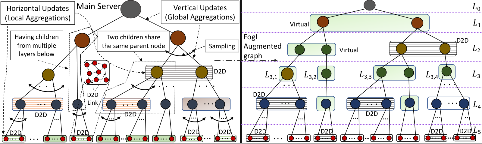
We consider the network architecture of FogL as depicted on the left in Fig. 3. In FogL, both inter-layer and intra-layer communications take place to conduct ML model training. The inter-layer communications are captured via a tree graph, with the main server at the root and end devices as the leaves. Each layer is partitioned into multiple clusters, with each device in a cluster sharing the same parent node in the next layer up. In general, each node may have a parent node located multiple layers above (e.g., an edge device can be directly connected to an edge server), and multiple clusters can share the same parent node (e.g., multiple groups of cellular devices share the same BS). Except at the bottom layer, each node in the hierarchy is the parent for a subset of the nodes, and is responsible for gathering the model parameters of its children nodes.

From this FogL network representation, we construct the FogL augmented network graph shown on the right of Fig. 3, where several virtual nodes and clusters have been added. Virtual nodes are added in such a way that each node has a single parent node in its immediate upper layer. Also, when multiple clusters share the same parent node, a layer is added to the FogL augmented graph that consists of multiple intermediate virtual nodes forming a virtual cluster, such that there is always a one-to-one mapping between the clusters and parent nodes. If necessary, the nodes in the highest layer before the main server will form a virtual cluster to preserve this one-to-one mapping. A node without any neighbors in its layer is also assumed to form a virtual singleton cluster. For convenience, we refer to the structure of Fig. 3 as a tree since in macro-scale it resembles a tree structure. However, in the micro-scale, nodes inside the clusters form connected graphs through which D2D communications are performed, differentiating the structure from a tree graph.

The FogL augmented graph has the following properties: (i) each parent node has a single cluster associated with it in the layer immediately below it; (ii) the length of the paths from the root to each of the leaf nodes are the same; and (iii) the layer below the root always consists of one cluster. The network consists of $|\mathcal{L}|+1$ layers, where $\mathcal{L}\triangleq\{L_{1},\cdots,L_{|\mathcal{L}|}\}$ denotes the set of layers below the server. The root/server is located at ${L}_{0}$ and the end devices are contained in ${L}_{|\mathcal{L}|}$. Inside layer ${L}_{j}$, $1\leq j\leq|\mathcal{L}|$, there exists a set of clusters indexed by ${L}_{j,1},{L}_{j,2},\cdots$ (see Fig. 3). We let the nodes move between the clusters in the same layer. To capture these dynamics, we use $\mathcal{L}^{(k)}_{j,i}$ (i.e., calligraphic font) to refer to the set of nodes inside cluster ${L}_{j,i}$ at learning iteration $k$ (described in Sec. II-B). For ease of presentation, we assume that the number of clusters at each layer is time invariant, i.e., each cluster always contains at least one node and nodes do not form new clusters. We let $\mathcal{N}_{j}$ denote the set of nodes in layer ${L}_{j}$ and $N_{j}\triangleq|\mathcal{N}_{j}|$.

For convenience, we will sometimes use ${C}$ to denote an arbitrary cluster (i.e., any ${L}_{j,i}$) and $\mathcal{C}^{(k)}$ (i.e., calligraphic font) to refer to its set of nodes at iteration $k$. We also sometimes use $n$ to denote an arbitrary node. For each node $n$ located in layers ${L}_{|\mathcal{L}|-1},\cdots,{L}_{0}$, we let ${Q}(n)$ denote the index of its child cluster and $\mathcal{Q}^{(k)}(n)$ denote the set of its children nodes (i.e., the nodes in $Q(n)$) at global iteration $k$.

Each end device $n$ is associated with a dataset $\mathcal{D}_{n}$. Each element $d_{i}\in\mathcal{D}_{n}$ of a dataset, called a training sample, is represented via a feature vector $\textbf{x}_{i}$ and a label $y_{i}$ for the ML task of interest. For example, in image classification, $\mathbf{x}_{i}$ may be the RGB colors of all pixels in the image, and $y_{i}$ may be the identity of the person in the image sample. The goal of the ML task is to learn the parameters $\mathbf{w}\in\mathbb{R}^{M}$ of a particular $M$-dimensional model (e.g., an SVM or a neural network) that are expected to maximize the accuracy in mapping from $\mathbf{x}_{i}$ to $y_{i}$ across any sample in the network. The model is associated with a loss $\widetilde{f}(\textbf{w},\textbf{x}_{i},y_{i})$, referred to as $\widetilde{f}_{i}(\textbf{w})$ for brevity, that quantifies the error of parameter realization $\mathbf{w}$ on $d_{i}$. We refer to Table 1 in [19] for a list of common ML loss functions.

The global loss of the ML model is formulated as

The value of $D$ in (5) is assumed to be known at the main server, since it only requires uplink transmission of the scalar $|\mathcal{D}_{n}|$ by each end device $n\in\mathcal{N}_{|\mathcal{L}|}$, which can be aggregated and propagated upstream by each parent node in the hierarchy. As we will see, our method does not require knowledge of each individual $|\mathcal{D}_{n}|$ at the server to conduct the parameter averaging given in (5), since the number of data points at each end device will be encapsulated in a scaled model parameter vector shared to its parent node (see Sec. III-B). On the downlink from the server to the edge devices, we assume that the (common) global parameter $\mathbf{w}^{(k-1)}$ can be readily shared through the hierarchy to reach to the end devices, e.g., through a broadcasting protocol. These devices will then conduct (3) and (4) locally. The challenge, then, is computing (5) at the main server. To do this, in federated learning, the devices will directly upload (4) to the server. However, this is prohibitive in a large-scale fog computing system. First, it may require high energy consumption: uplink transmissions from battery-limited devices to nodes at a higher layer typically correspond to long physical distances, and can deplete individual device batteries. Second, it may induce high network traffic and long latencies: a neural network with even hundreds of parameters, which would be small by today’s standards [24], would require transmission of billions of parameters in the upper layers during each iteration over a network with millions of nodes. Additionally, it may overload current cellular and vehicular architectures: these infrastructures are not designed to handle large jumps in the number of active users [43], which would be the case with simultaneous uplink transmissions at the bottom-most layer. These issues require a novel approach to parameter aggregations, which we develop in this paper.

The main server in FogL is only interested in the weighted average of the local parameters (5). Consequently, we propose local aggregations at each network layer. To achieve this, each cluster in Fig. 3 follows one of two mechanisms:

1. 1.

   Distributed aggregation: The nodes engage in a cooperative scheme facilitated by D2D communications to realize the consensus/average of their local model parameters. The parent node then samples parameters of one of the children and scales it by the number of children to calculate an approximate sum of the children nodes’ parameters.

2. 2.

   Instant aggregation: Each node instead uploads its local model to the parent node. The parent computes the aggregation directly as a sum of the children nodes’ parameters.

The communication requirement of the instant aggregation is often significantly higher than the distributed aggregation since D2D communications generally occur over much shorter distances, which makes them less power/energy consuming. We refer to mechanisms 1 and 2 mentioned above as limited uplink transmission (LUT) and extensive uplink transmission (EUT), respectively.¹¹ 1 We assume that each node belongs either to an EUT or to an LUT cluster. If some portion of the nodes in a cluster are capable of D2D communications while the rest are not, the cluster can be broken down into two clusters (i.e., an LUT and an EUT cluster) with the same parent node, based on which the fogL augmented network graph in Sec. II-A is then constructed. Not all clusters can operate in LUT mode, since not all are D2D enabled, e.g., due to sparse connections between devices. Still, we can expect significant advantages in terms of the volume of parameters uploaded through the system with a combination of EUT and LUT clusters, as depicted in Fig. 4. At the bottom layers where communication is mostly over the air, D2D can also be implemented through the out-band mode [44]. This has the additional advantage of not occupying the licensed spectrum, which results in bandwidth savings that can lead to an improved quality of service.

We allow a cluster to switch between EUT and LUT over time. For instance, the connectivity between a fleet of miniature UAVs will vary as they travel, necessitating EUT when D2D is not feasible. To capture this dynamic, for each cluster ${C}$, at global iteration $k$, $\mathbbm{1}^{(k)}_{\{{C}\}}$ captures the operating mode, which is $1$ if the cluster operates in LUT mode, and $0$ otherwise. In each LUT cluster, a node will only communicate with its neighboring devices, which may not include the whole cluster. Further, each node’s neighborhood may evolve over time. For example, when the communications are conducted over the air as in Fig. 2(2(a)), the neighbors in one aggregation interval are identified based on the distances among the nodes and their transmit powers. We will explicitly consider such evolutions in cluster topology in our distributed consensus model in Sec. III.

In the simple case where there is only one layer below the server, i.e., $|\mathcal{L}|=1$, consisting of a single EUT cluster, the FogL architecture reduces to federated learning. If instead there is just one layer of one LUT cluster with no server, FogL resembles fully distributed learning [29, 28, 17]. One of our contributions is developing and analyzing this generalized cluster-based multi-layer hybrid learning paradigm for FogL.

Note that the parameter update in (5) can be written as

This asserts that the global parameters can also be obtained via the gradients of the devices, implying that the devices can either share their gradients or their parameters during training. This equivalence arises from the one-step update in (4), which is a common assumption in federated learning [13, 14, 45]. However, recent work [19, 21] has advocated conducting multiple rounds of local updates between global aggregations to reduce communication costs; in this case, the parameters are required for each aggregation. In this paper, we focus on the more general case of parameter sharing, although we obtain one theoretical result (Proposition 3) based on gradient sharing.

In LUT clusters, devices leverage D2D communications to obtain an approximate value of the average of their parameters. A basic approach would be to implement a message passing algorithm where nodes exchange parameters with their neighbors until each node in the cluster has all parameters stored locally. Each node can then readily calculate the aggregated value, and one of them can be sampled by the parent node. Collecting a table of parameters at each node may not be feasible, however, given how large these vectors can be for contemporary ML models, as discussed in Sec. II-B. Instead, we desire a technique that (i) does not require any node to store a table of all model parameters in the cluster, (ii) can be implemented in a distributed manner via D2D, and (iii) is generalizable across different network layers. In the following, we leverage distributed average consensus methods for this.

Referring to Fig. 3, during each iteration $k$ of training, the LUT clusters engage in D2D communications, where each node desires estimating the average value of the parameters inside its cluster. For each cluster ${C}$ that is LUT during the $k$th global aggregation iteration (i.e., for which $\mathbbm{1}^{(k)}_{\{{C}\}}=1$), we let $G^{(k)}_{{C}}=\big(\mathcal{C}^{(k)},\mathcal{E}^{(k)}_{{C}}\big)$ denote its communication graph. In this graph, $\mathcal{C}^{(k)}$ is the set of nodes belonging to the cluster, and there is an edge $(m,n)\in\mathcal{E}^{(k)}_{{C}}$ between nodes $m,n\in\mathcal{C}^{(k)}$ iff they can communicate via D2D during $k$. We assume that $G^{(k)}_{{C}}$ is undirected, connected, and static for the duration of one iteration $k$, although it may vary in different iterations. Note that we have abstracted the physical layer wireless/wired communication medium of each LUT cluster $C$ to a general graph topology $G_{C}^{(k)}$. In a wireless cluster, different channel conditions and communication configurations among the devices will manifest as different topologies for $G_{C}^{(k)}$.

We employ the family of linear distributed consensus algorithms [46], where during the global iteration $k$, the nodes inside LUT cluster ${C}$ conduct $\theta^{(k)}_{{C}}\in\mathbb{N}$ rounds of D2D (number of D2D rounds is a design parameter obtained in Sec. III-C). Each round of D2D consists of parameter transfers between neighboring nodes. Formally, during global iteration $k$, each node $n\in\mathcal{C}^{(k)}$ engages in the following rounds of iterative updates for $t=0,...,\theta^{(k)}_{{C}}-1$:

Due to time constraints (i.e., depending on the required time between global aggregations), the number of D2D rounds cannot be arbitrarily large, and thus the nodes inside a cluster often do not have a perfect estimate of the average value of their parameters. In Sec. III-C, we analyze the effect of a finite number of D2D rounds on the MH-FL performance.

In the following, we introduce a scaled parameter for each node $n$ denoted by $\widetilde{\mathbf{w}}_{n}$ and develop an approach to perform global aggregations based on manipulation and relaying of these parameters across different layers of the network. The definition of $\widetilde{\mathbf{w}}_{n}$ depends on the layer where node $n$ is located.

One of the key contributions of MH-FL is the integration of D2D communications with multi-layer parameter transfers. As discussed, D2D communications are conducted through time varying topology structures among the nodes, which introduce a network dimension to model training. Studying this effect under limited D2D rounds regime is the main theme of our theoretical analysis. Before presenting our main results, we first introduce a few assumptions and a definition. Henceforth, $\|.\|$ denotes the 2-norm unless otherwise stated.

The above properties are common assumptions in federated learning and ML literature [45, 13, 47, 48, 49]. Commonly encountered ML models with convex loss functions are linear regression, logistic regression, squared SVM, and single layer neural networks with convex activation functions. In practice, these models are implemented with an additional regularization term to improve the convergence and avoid model overfitting, which makes them strongly convex [49]. We will conduct our convergence analysis based on this assumption and design control algorithms in Sec. III-D for both the convex (Algorithm 2) and non-convex (Algorithm 3) cases.

We will also find it useful to write the consensus algorithm in matrix form. Letting $\widetilde{\mathbf{W}}^{(k)}_{{C}}\in\mathbb{R}^{|\mathcal{C}^{(k)}|\times M}$ denote the matrix of scaled parameters across all nodes in an LUT cluster ${C}$ prior to consensus in iteration $k$, the evolution of the nodes’ parameters described by (9) can be written as

In Assumption 2, $\lambda^{(k)}_{{C}}$ can be interpreted as an upper bound on the spectral radius, which plays a key role in our results.

At the bottom-most layer, the above defined quantity is indicative of the degree of data heterogeneity (i.e., the level of non-i.i.d) among the nodes in a cluster, whereas in the upper layers it captures the heterogeneity of data contained in sub-trees with their roots being the nodes in the cluster. We show in Theorem 1 how it impacts the convergence bound, and in the subsequent results how it dictates the number of D2D rounds. Then, in Sec. III-D, we develop control algorithms that approximate the divergence in a distributed manner at every cluster, and use it to control the convergence rate.

With all else constant, fewer rounds of D2D results in lower power consumption and network load among the devices in LUT clusters. Motivated by this, we develop control algorithms for MH-FL that tune the number of D2D rounds through time (global aggregations) and space (network layers).

References

• [1] D. Ciregan, U. Meier, and J. Schmidhuber, “Multi-column deep neural networks for image classification,” in Proc. IEEE Conf. Comput. Vision Pattern Recog. (CVPR), 2012, pp. 3642–3649.
• [2] R. Collobert and J. Weston, “A unified architecture for natural language processing: Deep neural networks with multitask learning,” in Proc. Int. Conf. Mach. Learn., 2008, pp. 160–167.
• [3] B. McMahan, E. Moore, D. Ramage, S. Hampson, and B. A. y Arcas, “Communication-efficient learning of deep networks from decentralized data,” in Proc. Artif. Intell. Stat., 2017, pp. 1273–1282.
• [4] S. Hosseinalipour, C. G. Brinton, V. Aggarwal, H. Dai, and M. Chiang, “From federated to fog learning: Distributed machine learning over heterogeneous wireless networks,” IEEE Commun. Mag., vol. 58, no. 12, pp. 41–47, 2020.
• [5] M. Chiang, S. Ha, F. Risso, T. Zhang, and I. Chih-Lin, “Clarifying fog computing and networking: 10 questions and answers,” IEEE Commun. Mag., vol. 55, no. 4, pp. 18–20, 2017.
• [6] M. N. Tehrani, M. Uysal, and H. Yanikomeroglu, “Device-to-device communication in 5G cellular networks: challenges, solutions, and future directions,” IEEE Commun. Mag., vol. 52, no. 5, pp. 86–92, 2014.
• [7] M. Abolhasan, T. Wysocki, and E. Dutkiewicz, “A review of routing protocols for mobile ad hoc networks,” Ad hoc Netw., vol. 2, no. 1, pp. 1–22, 2004.
• [8] S. Zeadally, R. Hunt, Y.-S. Chen, A. Irwin, and A. Hassan, “Vehicular ad hoc networks (VANETS): status, results, and challenges,” Telecommun. Syst., vol. 50, no. 4, pp. 217–241, 2012.
• [9] I. Bekmezci, O. K. Sahingoz, and Ş. Temel, “Flying ad-hoc networks (FANETs): A survey,” Ad hoc Netw., vol. 11, no. 3, pp. 1254–1270, 2013.
• [10] K. Akkaya and M. Younis, “A survey on routing protocols for wireless sensor networks,” Ad hoc Netw., vol. 3, no. 3, pp. 325–349, 2005.
• [11] Y. Zhang, D. J. Love, J. V. Krogmeier, C. R. Anderson, R. W. Heath, and D. R. Buckmaster, “Challenges and opportunities of future rural wireless communications,” IEEE Commun. Mag., 2021.
• [12] S. Maheshwari, D. Raychaudhuri, I. Seskar, and F. Bronzino, “Scalability and performance evaluation of edge cloud systems for latency constrained applications,” in IEEE/ACM Symp. Edge Comput., 2018, pp. 286–299.
• [13] M. Chen, Z. Yang, W. Saad, C. Yin, H. V. Poor, and S. Cui, “A joint learning and communications framework for federated learning over wireless networks,” arXiv preprint arXiv:1909.07972, 2019.
• [14] N. H. Tran, W. Bao, A. Zomaya, M. N. H. Nguyen, and C. S. Hong, “Federated learning over wireless networks: Optimization model design and analysis,” in Proc. IEEE Int. Conf. Comput. Commun. (INFOCOM), 2019, pp. 1387–1395.
• [15] M. M. Amiri and D. Gündüz, “Federated learning over wireless fading channels,” IEEE Trans. Wireless Commun., vol. 19, no. 5, pp. 3546–3557, 2020.
• [16] N. Shlezinger, M. Chen, Y. C. Eldar, H. V. Poor, and S. Cui, “Federated learning with quantization constraints,” in Proc. IEEE Int. Conf. Acoustics, Speech, Signal Process. (ICASSP), 2020, pp. 8851–8855.
• [17] C.-S. Lee, N. Michelusi, and G. Scutari, “Finite-bit quantization for distributed algorithms with linear convergence,” arXiv preprint arXiv:2107.11304, 2021.
• [18] C. Renggli, S. Ashkboos, M. Aghagolzadeh, D. Alistarh, and T. Hoefler, “SparCML: High-performance sparse communication for machine learning,” in Proc. Int. Conf. High Perform. Comput., Netw., Storage Anal., 2019, pp. 1–15.
• [19] S. Wang, T. Tuor, T. Salonidis, K. K. Leung, C. Makaya, T. He, and K. Chan, “Adaptive federated learning in resource constrained edge computing systems,” IEEE J. Sel. Areas Commun. (JSAC), vol. 37, no. 6, pp. 1205–1221, 2019.
• [20] D. Ye, R. Yu, M. Pan, and Z. Han, “Federated learning in vehicular edge computing: A selective model aggregation approach,” IEEE Access, vol. 8, pp. 23 920–23 935, 2020.
• [21] Y. Tu, Y. Ruan, S. Wang, S. Wagle, C. G. Brinton, and C. Joe-Wang, “Network-aware optimization of distributed learning for fog computing,” in Proc. IEEE Int. Conf. Comput. Commun. (INFOCOM), 2020.
• [22] S. Wang, M. Lee, S. Hosseinalipour, R. Morabito, M. Chiang, and C. G. Brinton, “Device sampling for heterogeneous federated learning: Theory, algorithms, and implementation,” in IEEE Conf. Comput. Commun. (INFOCOM), 2021, pp. 1–10.
• [23] S. Ji, W. Jiang, A. Walid, and X. Li, “Dynamic sampling and selective masking for communication-efficient federated learning,” arXiv preprint arXiv:2003.09603, 2020.
• [24] W. Wang, Y. Sun, B. Eriksson, W. Wang, and V. Aggarwal, “Wide compression: Tensor ring nets,” in Proc. IEEE Conf. Comput. Vision Pattern Recog. (CVPR), 2018, pp. 9329–9338.
• [25] L. Liu, J. Zhang, S. Song, and K. B. Letaief, “Client-edge-cloud hierarchical federated learning,” in Proc. IEEE Int. Conf. Commun. (ICC), 2020, pp. 1–6.
• [26] S. Luo, X. Chen, Q. Wu, Z. Zhou, and S. Yu, “HFEL: Joint edge association and resource allocation for cost-efficient hierarchical federated edge learning,” IEEE Trans. Wireless Commun., pp. 1–1, 2020.
• [27] M. S. H. Abad, E. Ozfatura, D. GUndUz, and O. Ercetin, “Hierarchical federated learning across heterogeneous cellular networks,” in Proc. IEEE ICASSP, 2020, pp. 8866–8870.
• [28] S. Savazzi, M. Nicoli, and V. Rampa, “Federated learning with cooperating devices: A consensus approach for massive IoT networks,” IEEE Internet Things J., vol. 7, no. 5, pp. 4641–4654, 2020.
• [29] C. Hu, J. Jiang, and Z. Wang, “Decentralized federated learning: A segmented gossip approach,” arXiv preprint arXiv:1908.07782, 2019.
• [30] A. Elgabli, J. Park, A. S. Bedi, M. Bennis, and V. Aggarwal, “GADMM: Fast and communication efficient framework for distributed machine learning,” arXiv preprint arXiv:1909.00047, 2019.
• [31] V. Smith, S. Forte, C. Ma, M. Takáč, M. I. Jordan, and M. Jaggi, “CoCoA: A general framework for communication-efficient distributed optimization,” J. Mach. Learn. Res., vol. 18, no. 1, pp. 8590–8638, 2017.
• [32] P. Richtárik and M. Takáč, “Distributed coordinate descent method for learning with big data,” J. Mach. Learn. Res., vol. 17, no. 1, pp. 2657–2681, 2016.
• [33] S. Niknam, H. S. Dhillon, and J. H. Reed, “Federated learning for wireless communications: Motivation, opportunities and challenges,” arXiv preprint arXiv:1908.06847, 2019.
• [34] G. Zhu, D. Liu, Y. Du, C. You, J. Zhang, and K. Huang, “Toward an intelligent edge: Wireless communication meets machine learning,” IEEE Commun. Mag., vol. 58, no. 1, pp. 19–25, 2020.
• [35] C. L. P. Chen, G. Wen, Y. Liu, and F. Wang, “Adaptive consensus control for a class of nonlinear multiagent time-delay systems using neural networks,” IEEE Trans. Neural Netw. Learning Syst., vol. 25, no. 6, pp. 1217–1226, 2014.
• [36] T. Li and J.-F. Zhang, “Consensus conditions of multi-agent systems with time-varying topologies and stochastic communication noises,” IEEE Trans. Autom. Control, vol. 55, no. 9, pp. 2043–2057, 2010.
• [37] S. Kar and J. M. F. Moura, “Distributed consensus algorithms in sensor networks with imperfect communication: Link failures and channel noise,” IEEE Trans. Signal Process., vol. 57, no. 1, pp. 355–369, 2009.
• [38] S. Manfredi, “Design of a multi-hop dynamic consensus algorithm over wireless sensor networks,” Control Eng. Practice, vol. 21, no. 4, pp. 381–394, 2013.
• [39] A. Nedic and A. Ozdaglar, “Distributed subgradient methods for multi-agent optimization,” IEEE Trans. Auto. Control, vol. 54, no. 1, pp. 48–61, 2009.
• [40] T. Chang, M. Hong, and X. Wang, “Multi-agent distributed optimization via inexact consensus ADMM,” IEEE Trans. Signal Process., vol. 63, no. 2, pp. 482–497, 2015.
• [41] T. Chang, A. Nedić, and A. Scaglione, “Distributed constrained optimization by consensus-based primal-dual perturbation method,” IEEE Trans. Autom. Control, vol. 59, no. 6, pp. 1524–1538, 2014.
• [42] B. Johansson, T. Keviczky, M. Johansson, and K. H. Johansson, “Subgradient methods and consensus algorithms for solving convex optimization problems,” in Proc. IEEE Conf. Decis. Control, 2008, pp. 4185–4190.
• [43] R. N. Clarke, “Expanding mobile wireless capacity: The challenges presented by technology and economics,” Telecommun. Policy, vol. 38, no. 8-9, pp. 693–708, 2014.
• [44] U. N. Kar and D. K. Sanyal, “An overview of device-to-device communication in cellular networks,” ICT Express, vol. 4, no. 4, pp. 203–208, 2018.
• [45] T. Zeng, O. Semiari, M. Mozaffari, M. Chen, W. Saad, and M. Bennis, “Federated learning in the sky: Joint power allocation and scheduling with UAV swarms,” arXiv preprint arXiv:2002.08196, 2020.
• [46] L. Xiao and S. Boyd, “Fast linear iterations for distributed averaging,” Syst. & Control Lett., vol. 53, no. 1, pp. 65–78, 2004.
• [47] A. Reisizadeh, A. Mokhtari, H. Hassani, A. Jadbabaie, and R. Pedarsani, “Fedpaq: A communication-efficient federated learning method with periodic averaging and quantization,” arXiv:1909.13014, 2019.
• [48] C. Dinh, N. H. Tran, M. N. Nguyen, C. S. Hong, W. Bao, A. Zomaya, and V. Gramoli, “Federated learning over wireless networks: Convergence analysis and resource allocation,” arXiv preprint arXiv:1910.13067, 2019.
• [49] M. P. Friedlander and M. Schmidt, “Hybrid deterministic-stochastic methods for data fitting,” SIAM J. Sci. Comput., vol. 34, no. 3, pp. A1380–A1405, 2012.
• [50] L. Xiao, S. Boyd, and S.-J. Kim, “Distributed average consensus with least-mean-square deviation,” J. Parallel Distrib. Comput., vol. 67, no. 1, pp. 33–46, 2007.
• [51] X. Jia, “Wireless networks and random geometric graphs,” in Proc. Int. Symp. Parallel Arch. Alg. Netw., 2004, pp. 575–579.
• [52] M. Hmila, M. Fernández-Veiga, M. Rodríguez-Pérez, and S. Herrería-Alonso, “Energy efficient power and channel allocation in underlay device to multi device communications,” IEEE Trans. Commun., vol. 67, no. 8, pp. 5817–5832, 2019.
• [53] S. Dominic and L. Jacob, “Joint resource block and power allocation through distributed learning for energy efficient underlay D2D communication with rate guarantee,” Comput. Commun., 2020.
• [54] C. Xie, S. Koyejo, and I. Gupta, “Asynchronous federated optimization,” arXiv preprint arXiv:1903.03934, 2019.
• [55] B. T. Polyak, “Gradient methods for minimizing functionals,” Zh. Vychisl. Mat. Mat. Fiz, vol. 3, no. 4, pp. 643–653, 1963.
• [56] D. P. Bertsekas and J. N. Tsitsiklis, Neuro-dynamic programming. Athena Scientific, 1996.
Seyyedali Hosseinalipour (M’20) received his Ph.D. in EE from NCSU in 2020. He is currently a postdoctoral researcher at Purdue University.
Sheikh Shams Azam is a Ph.D. student at Purdue University. He received his B.Tech. in ECE from NITK, India in 2015.
Christopher G. Brinton (SM’20) is an Assistant Professor of ECE at Purdue University. He received his Ph.D. in EE from Princeton University in 2016.
Nicolò Michelusi (SM’19) received his Ph.D. in EE from University of Padova, Italy, in 2013. He is an Assistant Professor at Arizona State University.
Vaneet Aggarwal (SM’15) received his Ph.D. in EE from Princeton University in 2010. He is currently an Associate Professor at Purdue University.
David Love (F’15) is the Nick Trbovich Professor of ECE at Purdue University. He received the Ph.D. degree in EE from University of Texas at Austin in 2004.
Huaiyu Dai (F’17) received the Ph.D. degree in EE from Princeton University in 2002. He is currently a Professor of ECE at NCSU, holding the title of University Faculty Scholar.
Appendix A Proof of Theorem 1
Proof.
We carry out the proof in three parts: In part I, we obtain the convergence behavior of MH-FL given arbitrary aggregation errors at the sampled devices. In part II, we obtain the aggregation error caused by the D2D consensus process. Finally, in part III, we derive the final convergence bound.
A-A PART I: Convergence Bound for General Local Aggregation Error at the Sampled Nodes
We first aim to bound the per-iteration decrease of the gap between the function F⁡(𝐰(k))F(\mathbf{w}^{(k)}) and F⁡(𝐰∗)F(\mathbf{w}^{*}). Using the Taylor expansion and the η\eta-smoothness of function FF, the following quadratic upper-bound can be obtained:
F⁡(𝐰(k))≤\displaystyle F(\mathbf{w}^{(k)})\leq F(𝐰(k−1))+(𝐰(k)−𝐰(k−1))⊤∇F(𝐰(k−1))+η2‖𝐰(k)−𝐰(k−1)‖2,∀k.\displaystyle F(\mathbf{w}^{(k-1)})+(\mathbf{w}^{(k)}-\mathbf{w}^{(k-1)})^{\top}\nabla F(\mathbf{w}^{(k-1)})+\frac{\eta}{2}\left\lVert\mathbf{w}^{(k)}-\mathbf{w}^{(k-1)}\right\rVert^{2},\penalty\ \penalty\ \forall k. (31)
To find the relationship between w(k−1)\textbf{w}^{(k-1)} and w(k)\textbf{w}^{(k)}, we follow the procedure described in the main text. For parent node apa_{p}, let ap+1′a^{\prime}_{p+1} denote the corresponding sampled node, ∀p\forall p, e.g., in the following nested sums a|ℒ|′a^{\prime}_{|\mathcal{L}|} denotes the sampled node in the last layer by parent node a|ℒ|−1a_{|\mathcal{L}|-1} in its above layer. This corresponds to an arbitrary realization of the children sampling at different parent nodes. Let a1′a^{\prime}_{1} denote the sampled node by the main server in L1L_{1}. The model parameter of this node is given by
𝐰^a1′(k)=∑a1∈ℒ1,1(k)∑a2∈𝒬(k)​(a1)∑a3∈𝒬(k)​(a2)⋯∑a|ℒ|∈𝒬(k)​(a|ℒ|−1)|𝒟a|ℒ||𝐰(k−1)a|ℒ||ℒ1,1(k)|\displaystyle\widehat{\mathbf{w}}^{(k)}_{{a^{\prime}_{1}}}=\frac{\displaystyle\sum_{{a_{1}}\in\mathcal{L}^{(k)}_{{1},{1}}}\sum_{a_{2}\in\mathcal{Q}^{(k)}(a_{1})}\sum_{a_{3}\in\mathcal{Q}^{(k)}(a_{2})}\cdots\sum_{a_{|\mathcal{L}|}\in\mathcal{Q}^{(k)}({a_{|\mathcal{L}|-1}})}|\mathcal{D}_{a_{|\mathcal{L}|}}|\mathbf{w}^{(k-1)}_{{a_{|\mathcal{L}|}}}}{|\mathcal{L}^{(k)}_{{1},1}|} (32)
−∑a1∈ℒ1,1(k)∑a2∈𝒬(k)​(a1)∑a3∈𝒬(k)​(a2)⋯∑a|ℒ|∈𝒬(k)​(a|ℒ|−1)β|𝒟a|ℒ||∇fa|ℒ|(𝐰(k−1)a|ℒ|)|ℒ1,1(k)|\displaystyle-\frac{\displaystyle\sum_{{a_{1}}\in\mathcal{L}^{(k)}_{{1},{1}}}\sum_{a_{2}\in\mathcal{Q}^{(k)}(a_{1})}\sum_{a_{3}\in\mathcal{Q}^{(k)}(a_{2})}\cdots\sum_{a_{|\mathcal{L}|}\in\mathcal{Q}^{(k)}({a_{|\mathcal{L}|-1}})}\beta|\mathcal{D}_{a_{|\mathcal{L}|}}|\nabla f_{{a_{|\mathcal{L}|}}}(\mathbf{w}^{(k-1)}_{{a_{|\mathcal{L}|}}})}{|\mathcal{L}^{(k)}_{{1},1}|}
+∑a1∈ℒ1,1(k)∑a2∈𝒬(k)​(a1)∑a3∈𝒬(k)​(a2)⋯∑a|ℒ|−1∈𝒬(k)​(a|ℒ|−2)𝟙{Q⁡(a|ℒ|−1)}(k)​|𝒬(k)​(a|ℒ|−1)|​𝐜a|ℒ|′(k)|ℒ1,1(k)|\displaystyle+\sum_{{a_{1}}\in\mathcal{L}^{(k)}_{{1},{1}}}\sum_{a_{2}\in\mathcal{Q}^{(k)}(a_{1})}\sum_{a_{3}\in\mathcal{Q}^{(k)}(a_{2})}\cdots\sum_{a_{|\mathcal{L}|-1}\in\mathcal{Q}^{(k)}({a_{|\mathcal{L}|-2}})}\frac{\mathbbm{1}^{(k)}_{\left\{{{Q}(a_{|\mathcal{L}|-1})}\right\}}|\mathcal{Q}^{(k)}(a_{|\mathcal{L}|-1})|\mathbf{c}^{(k)}_{a^{\prime}_{|\mathcal{L}|}}}{|\mathcal{L}^{(k)}_{{1},1}|}
+∑a1∈ℒ1,1(k)∑a2∈𝒬(k)​(a1)∑a3∈𝒬(k)​(a2)⋯∑a|ℒ|−2∈𝒬(k)​(a|ℒ|−3)𝟙{Q⁡(a|ℒ|−2)}(k)​|𝒬(k)​(a|ℒ|−2)|​𝐜a|ℒ|−1′(k)|ℒ1,1(k)|+\displaystyle+\sum_{{a_{1}}\in\mathcal{L}^{(k)}_{{1},{1}}}\sum_{a_{2}\in\mathcal{Q}^{(k)}(a_{1})}\sum_{a_{3}\in\mathcal{Q}^{(k)}(a_{2})}\cdots\sum_{a_{|\mathcal{L}|-2}\in\mathcal{Q}^{(k)}({a_{|\mathcal{L}|-3}})}\frac{\mathbbm{1}^{(k)}_{\left\{{{Q}(a_{|\mathcal{L}|-2})}\right\}}|\mathcal{Q}^{(k)}(a_{|\mathcal{L}|-2})|\mathbf{c}^{(k)}_{a^{\prime}_{|\mathcal{L}|-1}}}{|\mathcal{L}^{(k)}_{{1},1}|}+
+∑a1∈ℒ1,1(k)𝟙{Q⁡(a1)}(k)​|𝒬(k)​(a1)|​𝐜a2′(k)|ℒ1,1(k)|+𝟙(k){L1,1}𝐜(k)a1′,\displaystyle+\sum_{a_{1}\in\mathcal{L}^{(k)}_{{1},1}}\frac{\mathbbm{1}^{(k)}_{\left\{{{Q}(a_{1})}\right\}}|\mathcal{Q}^{(k)}(a_{1})|\mathbf{c}^{(k)}_{a^{\prime}_{2}}}{|\mathcal{L}^{(k)}_{{1},1}|}+\mathbbm{1}^{(k)}_{\left\{{{L}_{{1},1}}\right\}}\mathbf{c}^{(k)}_{a^{\prime}_{1}},
which the main server uses to obtain the next global parameter as follows (due to the existence of the indicator function in the last term of the above expression, the following expression holds regardless of the operating mode of the cluster at layer L1{L}_{1}):
w(k)=|ℒ1,1(k)|​𝐰^a1′(k)D.\textbf{w}^{(k)}=\frac{|\mathcal{L}^{(k)}_{{1},1}|{\widehat{\mathbf{w}}}^{(k)}_{{a^{\prime}_{1}}}}{D}. (33)
Based on (3), it can be verified that
∑a1∈ℒ1,1(k)∑a2∈𝒬(k)​(a1)∑a3∈𝒬(k)​(a2)⋯∑a|ℒ|∈𝒬(k)​(a|ℒ|−1)|𝒟a|ℒ||𝐰(k−1)a|ℒ|=Dw(k−1).\displaystyle\displaystyle\sum_{{a_{1}}\in\mathcal{L}^{(k)}_{{1},{1}}}\sum_{a_{2}\in\mathcal{Q}^{(k)}(a_{1})}\sum_{a_{3}\in\mathcal{Q}^{(k)}(a_{2})}\cdots\sum_{a_{|\mathcal{L}|}\in\mathcal{Q}^{(k)}({a_{|\mathcal{L}|-1}})}|\mathcal{D}_{a_{|\mathcal{L}|}}|\mathbf{w}^{(k-1)}_{{a_{|\mathcal{L}|}}}=D\textbf{w}^{(k-1)}. (34)
Also, using (1), we have
∑a1∈ℒ1,1(k)∑a2∈𝒬(k)​(a1)∑a3∈𝒬(k)​(a2)⋯∑a|ℒ|∈𝒬(k)​(a|ℒ|−1)β|𝒟a|ℒ||∇fa|ℒ|(𝐰(k−1)a|ℒ|)=βD∇F(w(k−1)).\displaystyle{\displaystyle\sum_{{a_{1}}\in\mathcal{L}^{(k)}_{{1},{1}}}\sum_{a_{2}\in\mathcal{Q}^{(k)}(a_{1})}\sum_{a_{3}\in\mathcal{Q}^{(k)}(a_{2})}\cdots\sum_{a_{|\mathcal{L}|}\in\mathcal{Q}^{(k)}({a_{|\mathcal{L}|-1}})}\beta|\mathcal{D}_{a_{|\mathcal{L}|}}|\nabla f_{{a_{|\mathcal{L}|}}}(\mathbf{w}^{(k-1)}_{{a_{|\mathcal{L}|}}})}=\beta D\nabla F(\textbf{w}^{(k-1)}). (35)
Replacing the above two equations in (32) and performing the update given by (33), we get
w(k)=w(k−1)−β∇F(w(k−1))+1D(∑a1∈ℒ1,1(k)∑a2∈𝒬(k)​(a1)∑a3∈𝒬(k)​(a2)⋯∑a|ℒ|−1∈𝒬(k)​(a|ℒ|−2)𝟙(k){Q⁡(a|ℒ|−1)}|𝒬(k)(a|ℒ|−1)|𝐜(k)a|ℒ|′\displaystyle{\displaystyle\textbf{w}}^{(k)}=\textbf{w}^{(k-1)}-\beta\nabla F(\textbf{w}^{(k-1)})+\frac{1}{D}\Bigg(\sum_{{a_{1}}\in\mathcal{L}^{(k)}_{{1},{1}}}\sum_{a_{2}\in\mathcal{Q}^{(k)}(a_{1})}\sum_{a_{3}\in\mathcal{Q}^{(k)}(a_{2})}\cdots\sum_{a_{|\mathcal{L}|-1}\in\mathcal{Q}^{(k)}({a_{|\mathcal{L}|-2}})}{\mathbbm{1}^{(k)}_{\left\{{{Q}(a_{|\mathcal{L}|-1})}\right\}}|\mathcal{Q}^{(k)}(a_{|\mathcal{L}|-1})|\mathbf{c}^{(k)}_{a^{\prime}_{|\mathcal{L}|}}} (36)
+∑a1∈ℒ1,1(k)∑a2∈𝒬(k)​(a1)∑a3∈𝒬(k)​(a2)⋯∑a|ℒ|−2∈𝒬(k)​(a|ℒ|−3)𝟙(k){Q⁡(a|ℒ|−2)}|𝒬(k)(a|ℒ|−2)|𝐜(k)a|ℒ|−1′+\displaystyle+\sum_{{a_{1}}\in\mathcal{L}^{(k)}_{{1},{1}}}\sum_{a_{2}\in\mathcal{Q}^{(k)}(a_{1})}\sum_{a_{3}\in\mathcal{Q}^{(k)}(a_{2})}\cdots\sum_{a_{|\mathcal{L}|-2}\in\mathcal{Q}^{(k)}({a_{|\mathcal{L}|-3}})}{\mathbbm{1}^{(k)}_{\left\{{{Q}(a_{|\mathcal{L}|-2})}\right\}}|\mathcal{Q}^{(k)}(a_{|\mathcal{L}|-2})|\mathbf{c}^{(k)}_{a^{\prime}_{|\mathcal{L}|-1}}}+
+∑a1∈ℒ1,1(k)𝟙(k){Q⁡(a1)}|𝒬(k)(a1)|𝐜(k)a2′+𝟙(k){L1,1}|ℒ(k)1,1|𝐜(k)a1′),\displaystyle+\sum_{a_{1}\in\mathcal{L}^{(k)}_{{1},1}}{\mathbbm{1}^{(k)}_{\left\{{{Q}(a_{1})}\right\}}|\mathcal{Q}^{(k)}(a_{1})|\mathbf{c}^{(k)}_{a^{\prime}_{2}}}+\mathbbm{1}^{(k)}_{\left\{{{L}_{{1},1}}\right\}}|\mathcal{L}^{(k)}_{{1},1}|\mathbf{c}^{(k)}_{a^{\prime}_{1}}\Bigg),
Calculating w(k)−w(k−1)\textbf{w}^{(k)}-\textbf{w}^{(k-1)} using the above equation and replacing the result in (31) yields
F⁡(𝐰(k))−F⁡(𝐰(k−1))≤(η​β22−β)​‖∇F​(𝐰(k−1))‖2\displaystyle F(\mathbf{w}^{(k)})-F(\mathbf{w}^{(k-1)})\leq\left(\frac{\eta\beta^{2}}{2}-\beta\right)\left\lVert\nabla F(\mathbf{w}^{(k-1)})\right\rVert^{2} (37)
+(1−β​ηD)(∑a1∈ℒ1,1(k)∑a2∈𝒬(k)​(a1)∑a3∈𝒬(k)​(a2)⋯∑a|ℒ|−1∈𝒬(k)​(a|ℒ|−2)𝟙(k){Q⁡(a|ℒ|−1)}|𝒬(k)(a|ℒ|−1)|𝐜(k)a|ℒ|′\displaystyle+\left(\frac{1-\beta\eta}{D}\right)\Bigg(\sum_{{a_{1}}\in\mathcal{L}^{(k)}_{{1},{1}}}\sum_{a_{2}\in\mathcal{Q}^{(k)}(a_{1})}\sum_{a_{3}\in\mathcal{Q}^{(k)}(a_{2})}\cdots\sum_{a_{|\mathcal{L}|-1}\in\mathcal{Q}^{(k)}({a_{|\mathcal{L}|-2}})}{\mathbbm{1}^{(k)}_{\left\{{{Q}(a_{|\mathcal{L}|-1})}\right\}}|\mathcal{Q}^{(k)}(a_{|\mathcal{L}|-1})|\mathbf{c}^{(k)}_{a^{\prime}_{|\mathcal{L}|}}}
+∑a1∈ℒ1,1(k)∑a2∈𝒬(k)​(a1)∑a3∈𝒬(k)​(a2)⋯∑a|ℒ|−2∈𝒬(k)​(a|ℒ|−3)𝟙(k){Q⁡(a|ℒ|−2)}|𝒬(k)(a|ℒ|−2)|𝐜(k)a|ℒ|−1′+⋯\displaystyle+\sum_{{a_{1}}\in\mathcal{L}^{(k)}_{{1},{1}}}\sum_{a_{2}\in\mathcal{Q}^{(k)}(a_{1})}\sum_{a_{3}\in\mathcal{Q}^{(k)}(a_{2})}\cdots\sum_{a_{|\mathcal{L}|-2}\in\mathcal{Q}^{(k)}({a_{|\mathcal{L}|-3}})}{\mathbbm{1}^{(k)}_{\left\{{{Q}(a_{|\mathcal{L}|-2})}\right\}}|\mathcal{Q}^{(k)}(a_{|\mathcal{L}|-2})|\mathbf{c}^{(k)}_{a^{\prime}_{|\mathcal{L}|-1}}}+\cdots
+∑a1∈ℒ1,1(k)𝟙(k){Q⁡(a1)}|𝒬(k)(a1)|𝐜(k)a2′+𝟙(k){L1,1}|ℒ(k)1,1|𝐜(k)a1′)⊤∇F(𝐰(k−1))\displaystyle+\sum_{a_{1}\in\mathcal{L}^{(k)}_{{1},1}}{\mathbbm{1}^{(k)}_{\left\{{{Q}(a_{1})}\right\}}|\mathcal{Q}^{(k)}(a_{1})|\mathbf{c}^{(k)}_{a^{\prime}_{2}}}+\mathbbm{1}^{(k)}_{\left\{{{L}_{{1},1}}\right\}}|\mathcal{L}^{(k)}_{{1},1}|\mathbf{c}^{(k)}_{a^{\prime}_{1}}\Bigg)^{\top}\nabla F(\mathbf{w}^{(k-1)})
+η2​D2∥∑a1∈ℒ1,1(k)∑a2∈𝒬(k)​(a1)∑a3∈𝒬(k)​(a2)⋯∑a|ℒ|−1∈𝒬(k)​(a|ℒ|−2)𝟙(k){Q⁡(a|ℒ|−1)}|𝒬(k)(a|ℒ|−1)|𝐜(k)a|ℒ|′\displaystyle+\frac{\eta}{2D^{2}}\Big\|\sum_{{a_{1}}\in\mathcal{L}^{(k)}_{{1},{1}}}\sum_{a_{2}\in\mathcal{Q}^{(k)}(a_{1})}\sum_{a_{3}\in\mathcal{Q}^{(k)}(a_{2})}\cdots\sum_{a_{|\mathcal{L}|-1}\in\mathcal{Q}^{(k)}({a_{|\mathcal{L}|-2}})}{\mathbbm{1}^{(k)}_{\left\{{{Q}(a_{|\mathcal{L}|-1})}\right\}}|\mathcal{Q}^{(k)}(a_{|\mathcal{L}|-1})|\mathbf{c}^{(k)}_{a^{\prime}_{|\mathcal{L}|}}}
+∑a1∈ℒ1,1(k)𝟙(k){Q⁡(a1)}|𝒬(k)(a1)|𝐜(k)a2′+𝟙(k){L1,1}|ℒ(k)1,1|𝐜(k)a1′∥2.\displaystyle+\sum_{a_{1}\in\mathcal{L}^{(k)}_{{1},1}}{\mathbbm{1}^{(k)}_{\left\{{{Q}(a_{1})}\right\}}|\mathcal{Q}^{(k)}(a_{1})|\mathbf{c}^{(k)}_{a^{\prime}_{2}}}+\mathbbm{1}^{(k)}_{\left\{{{L}_{{1},1}}\right\}}|\mathcal{L}^{(k)}_{{1},1}|\mathbf{c}^{(k)}_{a^{\prime}_{1}}\Big\|^{2}.
Tuning the learning rate as β=1η\beta=\frac{1}{\eta}, we obtain
F⁡(𝐰(k))−F⁡(𝐰(k−1))≤−12​η​‖∇F​(𝐰(k−1))‖2+\displaystyle F(\mathbf{w}^{(k)})-F(\mathbf{w}^{(k-1)})\leq\frac{-1}{2\eta}\left\lVert\nabla F(\mathbf{w}^{(k-1)})\right\rVert^{2}+ (38)
η2​D2∥∑a1∈ℒ1,1(k)∑a2∈𝒬(k)​(a1)∑a3∈𝒬(k)​(a2)⋯∑a|ℒ|−1∈𝒬(k)​(a|ℒ|−2)𝟙(k){Q⁡(a|ℒ|−1)}|𝒬(k)(a|ℒ|−1)|𝐜(k)a|ℒ|′\displaystyle\frac{\eta}{2D^{2}}\Big\|\sum_{{a_{1}}\in\mathcal{L}^{(k)}_{{1},{1}}}\sum_{a_{2}\in\mathcal{Q}^{(k)}(a_{1})}\sum_{a_{3}\in\mathcal{Q}^{(k)}(a_{2})}\cdots\sum_{a_{|\mathcal{L}|-1}\in\mathcal{Q}^{(k)}({a_{|\mathcal{L}|-2}})}{\mathbbm{1}^{(k)}_{\left\{{{Q}(a_{|\mathcal{L}|-1})}\right\}}|\mathcal{Q}^{(k)}(a_{|\mathcal{L}|-1})|\mathbf{c}^{(k)}_{a^{\prime}_{|\mathcal{L}|}}}
Considering the right hand side of the above inequality, to bound ‖∇F​(𝐰(k−1))‖2\left\lVert\nabla F(\mathbf{w}^{(k-1)})\right\rVert^{2}, we use the strong convexity property of FF. Considering the strong convexity criterion in Assumption 1 with xx replaced by 𝐰(k−1)\mathbf{w}^{(k-1)} and minimizing the both hand sides, the minimum of the left hand side occurs at y=𝐰∗y=\mathbf{w}^{*} and the minimum of the right hand side occurs at y=𝐰(k−1)−1μ∇F(𝐰(k−1))y=\mathbf{w}^{(k-1)}-\frac{1}{\mu}\nabla F(\mathbf{w}^{(k-1)}). Replacing these values in the strong convexity criterion in Assumption 1 results in Polyak-Lojasiewicz inequality [55] in the following form:
‖∇F​(𝐰(k−1))‖2≥(F⁡(𝐰(k−1))−F⁡(𝐰∗))​2​μ,\left\lVert\nabla F(\mathbf{w}^{(k-1)})\right\rVert^{2}\geq(F(\mathbf{w}^{(k-1)})-F(\mathbf{w}^{*})){2\mu}, (39)
which yields
F⁡(𝐰(k))−F⁡(𝐰(k−1))≤−μη​(F⁡(𝐰(k−1))−F⁡(𝐰∗))+\displaystyle F(\mathbf{w}^{(k)})-F(\mathbf{w}^{(k-1)})\leq\frac{-\mu}{\eta}(F(\mathbf{w}^{(k-1)})-F(\mathbf{w}^{*}))+ (40)
η2​D2[∥∑a1∈ℒ1,1(k)∑a2∈𝒬(k)​(a1)∑a3∈𝒬(k)​(a2)⋯∑a|ℒ|−1∈𝒬(k)​(a|ℒ|−2)𝟙(k){Q⁡(a|ℒ|−1)}|𝒬(k)(a|ℒ|−1)|𝐜(k)a|ℒ|′\displaystyle\frac{\eta}{2D^{2}}\Bigg[\Big\|\sum_{{a_{1}}\in\mathcal{L}^{(k)}_{{1},{1}}}\sum_{a_{2}\in\mathcal{Q}^{(k)}(a_{1})}\sum_{a_{3}\in\mathcal{Q}^{(k)}(a_{2})}\cdots\sum_{a_{|\mathcal{L}|-1}\in\mathcal{Q}^{(k)}({a_{|\mathcal{L}|-2}})}{\mathbbm{1}^{(k)}_{\left\{{{Q}(a_{|\mathcal{L}|-1})}\right\}}|\mathcal{Q}^{(k)}(a_{|\mathcal{L}|-1})|\mathbf{c}^{(k)}_{a^{\prime}_{|\mathcal{L}|}}}
+∑a1∈ℒ1,1(k)𝟙(k){Q⁡(a1)}|𝒬(k)(a1)|𝐜(k)a2′+𝟙(k){L1,1}|ℒ(k)1,1|𝐜(k)a1′∥2].\displaystyle+\sum_{a_{1}\in\mathcal{L}^{(k)}_{{1},1}}{\mathbbm{1}^{(k)}_{\left\{{{Q}(a_{1})}\right\}}|\mathcal{Q}^{(k)}(a_{1})|\mathbf{c}^{(k)}_{a^{\prime}_{2}}}+\mathbbm{1}^{(k)}_{\left\{{{L}_{{1},1}}\right\}}|\mathcal{L}^{(k)}_{{1},1}|\mathbf{c}^{(k)}_{a^{\prime}_{1}}\Big\|^{2}\Bigg].
Then, we perform the following algebraic steps to bound the second term on the right hand side of the above inequality:
∥∑a1∈ℒ1,1(k)∑a2∈𝒬(k)​(a1)∑a3∈𝒬(k)​(a2)⋯∑a|ℒ|−1∈𝒬(k)​(a|ℒ|−2)𝟙(k){Q⁡(a|ℒ|−1)}|𝒬(k)(a|ℒ|−1)|𝐜(k)a|ℒ|′\displaystyle\Big\|\sum_{{a_{1}}\in\mathcal{L}^{(k)}_{{1},{1}}}\sum_{a_{2}\in\mathcal{Q}^{(k)}(a_{1})}\sum_{a_{3}\in\mathcal{Q}^{(k)}(a_{2})}\cdots\sum_{a_{|\mathcal{L}|-1}\in\mathcal{Q}^{(k)}({a_{|\mathcal{L}|-2}})}{\mathbbm{1}^{(k)}_{\left\{{{Q}(a_{|\mathcal{L}|-1})}\right\}}|\mathcal{Q}^{(k)}(a_{|\mathcal{L}|-1})|\mathbf{c}^{(k)}_{a^{\prime}_{|\mathcal{L}|}}} (41)
+∑a1∈ℒ1,1(k)𝟙(k){Q⁡(a1)}|𝒬(k)(a1)|𝐜(k)a2′+𝟙(k){L1,1}|ℒ(k)1,1|𝐜(k)a1′∥2\displaystyle+\sum_{a_{1}\in\mathcal{L}^{(k)}_{{1},1}}{\mathbbm{1}^{(k)}_{\left\{{{Q}(a_{1})}\right\}}|\mathcal{Q}^{(k)}(a_{1})|\mathbf{c}^{(k)}_{a^{\prime}_{2}}}+\mathbbm{1}^{(k)}_{\left\{{{L}_{{1},1}}\right\}}|\mathcal{L}^{(k)}_{{1},1}|\mathbf{c}^{(k)}_{a^{\prime}_{1}}\Big\|^{2}
≤(∥∑a1∈ℒ1,1(k)∑a2∈𝒬(k)​(a1)∑a3∈𝒬(k)​(a2)⋯∑a|ℒ|−1∈𝒬(k)​(a|ℒ|−2)𝟙(k){Q⁡(a|ℒ|−1)}|𝒬(k)(a|ℒ|−1)|𝐜(k)a|ℒ|′∥\displaystyle\leq\Bigg(\Big\|\sum_{{a_{1}}\in\mathcal{L}^{(k)}_{{1},{1}}}\sum_{a_{2}\in\mathcal{Q}^{(k)}(a_{1})}\sum_{a_{3}\in\mathcal{Q}^{(k)}(a_{2})}\cdots\sum_{a_{|\mathcal{L}|-1}\in\mathcal{Q}^{(k)}({a_{|\mathcal{L}|-2}})}{\mathbbm{1}^{(k)}_{\left\{{{Q}(a_{|\mathcal{L}|-1})}\right\}}|\mathcal{Q}^{(k)}(a_{|\mathcal{L}|-1})|\mathbf{c}^{(k)}_{a^{\prime}_{|\mathcal{L}|}}}\Big\|
+∥∑a1∈ℒ1,1(k)∑a2∈𝒬(k)​(a1)∑a3∈𝒬(k)​(a2)⋯∑a|ℒ|−2∈𝒬(k)​(a|ℒ|−3)𝟙(k){Q⁡(a|ℒ|−2)}|𝒬(k)(a|ℒ|−2)|𝐜(k)a|ℒ|−1′∥\displaystyle+\Big\|\sum_{{a_{1}}\in\mathcal{L}^{(k)}_{{1},{1}}}\sum_{a_{2}\in\mathcal{Q}^{(k)}(a_{1})}\sum_{a_{3}\in\mathcal{Q}^{(k)}(a_{2})}\cdots\sum_{a_{|\mathcal{L}|-2}\in\mathcal{Q}^{(k)}({a_{|\mathcal{L}|-3}})}{\mathbbm{1}^{(k)}_{\left\{{{Q}(a_{|\mathcal{L}|-2})}\right\}}|\mathcal{Q}^{(k)}(a_{|\mathcal{L}|-2})|\mathbf{c}^{(k)}_{a^{\prime}_{|\mathcal{L}|-1}}}\Big\|
+⋯\displaystyle+\cdots
OPEN+‖∑a1∈ℒ1,1(k)𝟙{Q⁡(a1)}(k)​|𝒬(k)​(a1)|​𝐜a2′(k)‖+‖𝟙{L1,1}(k)​|ℒ1,1(k)|​𝐜a1′(k)‖)2\displaystyle+\Big\|\sum_{a_{1}\in\mathcal{L}^{(k)}_{{1},1}}{\mathbbm{1}^{(k)}_{\left\{{{Q}(a_{1})}\right\}}|\mathcal{Q}^{(k)}(a_{1})|\mathbf{c}^{(k)}_{a^{\prime}_{2}}}\Big\|+\Big\|\mathbbm{1}^{(k)}_{\left\{{{L}_{{1},1}}\right\}}|\mathcal{L}^{(k)}_{{1},1}|\mathbf{c}^{(k)}_{a^{\prime}_{1}}\Big\|\Bigg)^{2}
≤(∑a1∈ℒ1,1(k)∑a2∈𝒬(k)​(a1)∑a3∈𝒬(k)​(a2)⋯∑a|ℒ|−1∈𝒬(k)​(a|ℒ|−2)𝟙(k){Q⁡(a|ℒ|−1)}|𝒬(k)(a|ℒ|−1)|∥𝐜(k)a|ℒ|′∥\displaystyle\leq\Bigg(\sum_{{a_{1}}\in\mathcal{L}^{(k)}_{{1},{1}}}\sum_{a_{2}\in\mathcal{Q}^{(k)}(a_{1})}\sum_{a_{3}\in\mathcal{Q}^{(k)}(a_{2})}\cdots\sum_{a_{|\mathcal{L}|-1}\in\mathcal{Q}^{(k)}({a_{|\mathcal{L}|-2}})}{\mathbbm{1}^{(k)}_{\left\{{{Q}(a_{|\mathcal{L}|-1})}\right\}}|\mathcal{Q}^{(k)}(a_{|\mathcal{L}|-1})|\Big\|\mathbf{c}^{(k)}_{a^{\prime}_{|\mathcal{L}|}}}\Big\|
+∑a1∈ℒ1,1(k)∑a2∈𝒬(k)​(a1)∑a3∈𝒬(k)​(a2)⋯∑a|ℒ|−2∈𝒬(k)​(a|ℒ|−3)𝟙(k){Q⁡(a|ℒ|−2)}|𝒬(k)(a|ℒ|−2)|∥𝐜(k)a|ℒ|−1′∥\displaystyle+\sum_{{a_{1}}\in\mathcal{L}^{(k)}_{{1},{1}}}\sum_{a_{2}\in\mathcal{Q}^{(k)}(a_{1})}\sum_{a_{3}\in\mathcal{Q}^{(k)}(a_{2})}\cdots\sum_{a_{|\mathcal{L}|-2}\in\mathcal{Q}^{(k)}({a_{|\mathcal{L}|-3}})}{\mathbbm{1}^{(k)}_{\left\{{{Q}(a_{|\mathcal{L}|-2})}\right\}}|\mathcal{Q}^{(k)}(a_{|\mathcal{L}|-2})|\Big\|\mathbf{c}^{(k)}_{a^{\prime}_{|\mathcal{L}|-1}}}\Big\|
+∑a1∈ℒ1,1(k)𝟙(k){Q⁡(a1)}|𝒬(k)(a1)|2∥𝐜(k)a2′∥+𝟙(k){L1,1}|ℒ(k)1,1|∥𝐜(k)a1′∥)2\displaystyle+\sum_{a_{1}\in\mathcal{L}^{(k)}_{{1},1}}{\mathbbm{1}^{(k)}_{\left\{{{Q}(a_{1})}\right\}}|\mathcal{Q}^{(k)}(a_{1})|^{2}\Big\|\mathbf{c}^{(k)}_{a^{\prime}_{2}}}\Big\|+\mathbbm{1}^{(k)}_{\left\{{{L}_{{1},1}}\right\}}|\mathcal{L}^{(k)}_{{1},1}|\Big\|\mathbf{c}^{(k)}_{a^{\prime}_{1}}\Big\|\Bigg)^{2}
≤(a)\displaystyle\overset{(a)}{\leq}
Φ[∑a1∈ℒ1,1(k)∑a2∈𝒬(k)​(a1)∑a3∈𝒬(k)​(a2)⋯∑a|ℒ|−1∈𝒬(k)​(a|ℒ|−2)𝟙(k){Q⁡(a|ℒ|−1)}|𝒬(k)(a|ℒ|−1)|2∥𝐜(k)a|ℒ|′∥2\displaystyle{\displaystyle\Phi}\Bigg[\sum_{{a_{1}}\in\mathcal{L}^{(k)}_{{1},{1}}}\sum_{a_{2}\in\mathcal{Q}^{(k)}(a_{1})}\sum_{a_{3}\in\mathcal{Q}^{(k)}(a_{2})}\cdots\sum_{a_{|\mathcal{L}|-1}\in\mathcal{Q}^{(k)}({a_{|\mathcal{L}|-2}})}{\mathbbm{1}^{(k)}_{\left\{{{Q}(a_{|\mathcal{L}|-1})}\right\}}|\mathcal{Q}^{(k)}(a_{|\mathcal{L}|-1})|^{2}\Big\|\mathbf{c}^{(k)}_{a^{\prime}_{|\mathcal{L}|}}}\Big\|^{2}
+∑a1∈ℒ1,1(k)∑a2∈𝒬(k)​(a1)∑a3∈𝒬(k)​(a2)⋯∑a|ℒ|−2∈𝒬(k)​(a|ℒ|−3)𝟙(k){Q⁡(a|ℒ|−2)}|𝒬(k)(a|ℒ|−2)|2∥𝐜(k)a|ℒ|−1′∥2\displaystyle+\sum_{{a_{1}}\in\mathcal{L}^{(k)}_{{1},{1}}}\sum_{a_{2}\in\mathcal{Q}^{(k)}(a_{1})}\sum_{a_{3}\in\mathcal{Q}^{(k)}(a_{2})}\cdots\sum_{a_{|\mathcal{L}|-2}\in\mathcal{Q}^{(k)}({a_{|\mathcal{L}|-3}})}{\mathbbm{1}^{(k)}_{\left\{{{Q}(a_{|\mathcal{L}|-2})}\right\}}|\mathcal{Q}^{(k)}(a_{|\mathcal{L}|-2})|^{2}\Big\|\mathbf{c}^{(k)}_{a^{\prime}_{|\mathcal{L}|-1}}}\Big\|^{2}
+∑a1∈ℒ1,1(k)𝟙(k){Q⁡(a1)}|𝒬(k)(a1)|2∥𝐜(k)a2′∥2+𝟙(k){L1,1}|ℒ(k)1,1|2∥𝐜(k)a1′∥2],\displaystyle+\sum_{a_{1}\in\mathcal{L}^{(k)}_{{1},1}}{\mathbbm{1}^{(k)}_{\left\{{{Q}(a_{1})}\right\}}|\mathcal{Q}^{(k)}(a_{1})|^{2}\Big\|\mathbf{c}^{(k)}_{a^{\prime}_{2}}}\Big\|^{2}+\mathbbm{1}^{(k)}_{\left\{{{L}_{{1},1}}\right\}}|\mathcal{L}^{(k)}_{{1},1}|^{2}\Big\|\mathbf{c}^{(k)}_{a^{\prime}_{1}}\Big\|^{2}\Bigg],
where the triangle inequality, e.g, for vectors ai, 1≤i≤n\textbf{a}_{i},\penalty\ 1\leq i\leq n: ‖∑i=1nai‖≤∑i=1n‖ai‖\left\lVert\sum_{i=1}^{n}\textbf{a}_{i}\right\rVert\leq\sum_{i=1}^{n}\left\lVert\textbf{a}_{i}\right\rVert, is applied sequentially and
Φ=N|ℒ|−1+N|ℒ|−2+⋯+N1+1.\Phi=N_{{|\mathcal{L}|-1}}+N_{{|\mathcal{L}|-2}}+\cdots+N_{{1}}+1. (42)
Also, inequality (a) in (41) is obtained by exploiting the Cauchy–Schwarz inequality,<a,a′>≤‖a‖.‖a′‖<\textbf{a},\textbf{a}^{\prime}>\penalty\ \leq\left\lVert\textbf{a}\right\rVert.\left\lVert\textbf{a}^{\prime}\right\rVert, which results in the following bound, where 𝐪=[q1,⋯,qb]\mathbf{q}=[q_{1},\cdots,q_{b}]:
(∑a=1bqi)2=(<𝟏,𝐪>)2≤b​∑a=1bqi2.\displaystyle\left(\sum_{a=1}^{b}q_{i}\right)^{2}=\left(<\mathbf{1},\mathbf{q}>\right)^{2}\leq b\sum_{a=1}^{b}q^{2}_{i}. (43)
A-B PART II: Finding the Consensus (local aggregation) Error in Each LUT Cluster
To further find each of the error terms in the right hand side of (41), we need to bound ‖𝐜ap′(k)‖2\Big\|\mathbf{c}^{(k)}_{{}{a^{\prime}_{p}}}\Big\|^{2}, 1≤p≤|ℒ|1\leq p\leq|\mathcal{L}|. For notations simplicity we consider bounding ‖𝐜a|ℒ|′(k)‖2\Big\|\mathbf{c}^{(k)}_{{a^{\prime}_{|\mathcal{L}|}}}\Big\|^{2} for the case where sampling is conducted from node a|ℒ|′a^{\prime}_{|\mathcal{L}|}, a|ℒ|′∈𝒞(k)a^{\prime}_{|\mathcal{L}|}\in\mathcal{C}^{(k)}, where LUT cluster C{C} is located in the bottom-most layer .
The evolution of nodes’ parameters during D2D communications in this cluster can be described by (12) as
𝐖^C(k)=(𝐕C(k))θC(k)​𝐖~C(k).\widehat{\mathbf{W}}_{{C}}^{(k)}=\left(\mathbf{V}^{(k)}_{{C}}\right)^{\theta^{(k)}_{{C}}}\widetilde{\mathbf{W}}_{{C}}^{(k)}. (44)
Let matrix 𝐖¯C(k)\overline{\mathbf{W}}_{{C}}^{(k)} denote the average of the vector of parameters in cluster C{C}. This matrix can be described as
𝐖¯C(k)=1|𝒞(k)|​1|𝒞(k)|⊤​𝐖~C(k)|𝒞(k)|.\overline{{\mathbf{W}}}_{{C}}^{(k)}=\frac{\textbf{1}_{|\mathcal{C}^{(k)}|}\textbf{1}_{|\mathcal{C}^{(k)}|}^{\top}{\widetilde{\mathbf{W}}}_{{C}}^{(k)}}{|\mathcal{C}^{(k)}|}. (45)
We next define the local aggregation error matrix 𝑬C(k)\bm{E}_{C}^{(k)} for cluster CC at the instance of global aggregation kk, which satisfies the following equality:
𝐄C(k)=𝐖^C(k)−𝐖¯C(k).\mathbf{E}_{C}^{(k)}=\widehat{\mathbf{W}}_{{C}}^{(k)}-\overline{\mathbf{W}}_{{C}}^{(k)}. (46)
Note that [𝐄C(k)]a′|ℒ|,:=𝐜a|ℒ|′(k)[\mathbf{E}_{C}^{(k)}]_{a^{\prime}_{|\mathcal{L}|},:}=\mathbf{c}^{(k)}_{a^{\prime}_{|\mathcal{L}|}}, where [𝐄C(k)]a′|ℒ|,:[\mathbf{E}_{C}^{(k)}]_{a^{\prime}_{|\mathcal{L}|},:} denotes the row describing the parameter of node a|ℒ|′a^{\prime}_{|\mathcal{L}|}. Note that 𝟏⊤​𝐄C(k)=𝟎\mathbf{1}^{\top}\mathbf{E}_{C}^{(k)}=\bm{0}, and thus (𝟏𝟏⊤)​𝐄C(k)=𝟎(\mathbf{1}\mathbf{1}^{\top})\mathbf{E}_{C}^{(k)}=\mathbf{0} and accordingly
𝐄C(k)\displaystyle\mathbf{E}_{C}^{(k)} =(𝐈−𝟏𝟏⊤|𝒞(k)|)​𝐄C(k)=(𝐈−𝟏𝟏⊤|𝒞(k)|)​(𝐖^C(k)−𝐖¯C(k))\displaystyle=\left(\mathbf{I}-\frac{\mathbf{1}\mathbf{1}^{\top}}{|\mathcal{C}^{(k)}|}\right)\mathbf{E}_{C}^{(k)}=\left(\mathbf{I}-\frac{\mathbf{1}\mathbf{1}^{\top}}{|\mathcal{C}^{(k)}|}\right)\left(\widehat{\mathbf{W}}_{{C}}^{(k)}-\overline{\mathbf{W}}_{{C}}^{(k)}\right) (47)
=(𝐈−𝟏𝟏⊤|𝒞(k)|)​((𝐕C(k))θC(k)​𝐖~C(k)−𝐖¯C(k))=(𝐈−𝟏𝟏⊤|𝒞(k)|)​((𝐕C(k))θC(k)​𝐖~C(k)−(𝐕C(k))θC(k)​𝐖¯C(k))\displaystyle=\left(\mathbf{I}-\frac{\mathbf{1}\mathbf{1}^{\top}}{|\mathcal{C}^{(k)}|}\right)\left(\left(\mathbf{V}^{(k)}_{{C}}\right)^{\theta^{(k)}_{{C}}}\widetilde{\mathbf{W}}_{{C}}^{(k)}-\overline{\mathbf{W}}_{{C}}^{(k)}\right)=\left(\mathbf{I}-\frac{\mathbf{1}\mathbf{1}^{\top}}{|\mathcal{C}^{(k)}|}\right)\left(\left(\mathbf{V}^{(k)}_{{C}}\right)^{\theta^{(k)}_{{C}}}\widetilde{\mathbf{W}}_{{C}}^{(k)}-\left(\mathbf{V}^{(k)}_{{C}}\right)^{\theta^{(k)}_{{C}}}\overline{\mathbf{W}}_{{C}}^{(k)}\right)
=((𝐕C(k))θC(k)−𝟏𝟏⊤|𝒞(k)|)​(𝐖~C(k)−𝐖¯C(k)),\displaystyle=\left(\left(\mathbf{V}^{(k)}_{{C}}\right)^{\theta^{(k)}_{{C}}}-\frac{\mathbf{1}\mathbf{1}^{\top}}{|\mathcal{C}^{(k)}|}\right)\left(\widetilde{\mathbf{W}}_{{C}}^{(k)}-\overline{\mathbf{W}}_{{C}}^{(k)}\right),
where 𝐈\mathbf{I} denotes the identity matrix. In the above equalities we have used the facts that (i) (𝐕C(k))θC(k)​𝐖¯C(k)=𝐖¯C(k)\left(\mathbf{V}^{(k)}_{{C}}\right)^{\theta^{(k)}_{{C}}}\overline{\mathbf{W}}_{{C}}^{(k)}=\overline{\mathbf{W}}_{{C}}^{(k)} since performing consensus on averaged matrix does not change the resulting parameters, and (ii) 𝟏𝟏⊤|𝒞(k)|​(𝐕C(k))θC(k)=𝟏𝟏⊤|𝒞(k)|\frac{\mathbf{1}\mathbf{1}^{\top}}{|\mathcal{C}^{(k)}|}\left(\mathbf{V}^{(k)}_{{C}}\right)^{\theta^{(k)}_{{C}}}=\frac{\mathbf{1}\mathbf{1}^{\top}}{|\mathcal{C}^{(k)}|} according to Assumption 2 since (𝐕C(k))θC(k)\left(\mathbf{V}^{(k)}_{{C}}\right)^{\theta^{(k)}_{{C}}} is also double stochastic.
Using the above properties, we finally bound ‖𝐜a|ℒ|′(k)‖\|\mathbf{c}^{(k)}_{a^{\prime}_{|\mathcal{L}|}}\| as follows:
‖𝐜a|ℒ|′(k)‖2\displaystyle\big\|\mathbf{c}^{(k)}_{a^{\prime}_{|\mathcal{L}|}}\big\|^{2} ≤trace​((𝐄C(k))⊤​𝐄C(k))=trace​((𝐖~C(k)−𝐖¯C(k))⊤​((𝐕C(k))θC(k)−𝟏𝟏⊤|𝒞(k)|)2​(𝐖~C(k)−𝐖¯C(k)))\displaystyle\leq\textrm{trace}\left((\mathbf{E}_{C}^{(k)})^{\top}\mathbf{E}_{C}^{(k)}\right)=\textrm{trace}\left(\left(\widetilde{\mathbf{W}}_{{C}}^{(k)}-\overline{\mathbf{W}}_{{C}}^{(k)}\right)^{\top}\left(\left(\mathbf{V}^{(k)}_{{C}}\right)^{\theta^{(k)}_{{C}}}-\frac{\mathbf{1}\mathbf{1}^{\top}}{|\mathcal{C}^{(k)}|}\right)^{2}\left(\widetilde{\mathbf{W}}_{{C}}^{(k)}-\overline{\mathbf{W}}_{{C}}^{(k)}\right)\right) (48)
≤(λC(k))2​θC(k)​∑q∈𝒞(k)‖𝐰~q(k)−𝐰¯C(k)‖2≤(λC(k))2​θC(k)​1|𝒞(k)|​∑q,q′∈𝒞(k)‖𝐰~q(k)−𝐰¯q′(k)‖2\displaystyle\leq(\lambda^{(k)}_{C})^{2\theta_{C}^{(k)}}\sum_{q\in\mathcal{C}^{(k)}}\|\widetilde{\mathbf{w}}^{(k)}_{{q}}-\overline{\mathbf{w}}^{(k)}_{C}\big\|^{2}\leq(\lambda^{(k)}_{C})^{2\theta_{C}^{(k)}}\frac{1}{|\mathcal{C}^{(k)}|}\sum_{q,q^{\prime}\in\mathcal{C}^{(k)}}\|\widetilde{\mathbf{w}}^{(k)}_{{q}}-\overline{\mathbf{w}}^{(k)}_{q^{\prime}}\big\|^{2}
≤(λC(k))2​θC(k)|𝒞(k)|maxq,q′∈𝒞(k)⁡‖𝐰~q(k)−𝐰¯q′(k)‖2≤(λC(k))2​θC(k)​|𝒞(k)|​(ΥC(k))2,\displaystyle\leq(\lambda^{(k)}_{C})^{2\theta_{C}^{(k)}}{|\mathcal{C}^{(k)}|}\max_{q,q^{\prime}\in\mathcal{C}^{(k)}}\|\widetilde{\mathbf{w}}^{(k)}_{{q}}-\overline{\mathbf{w}}^{(k)}_{q^{\prime}}\big\|^{2}\leq(\lambda^{(k)}_{C})^{2\theta_{C}^{(k)}}{|\mathcal{C}^{(k)}|}\left(\Upsilon_{C}^{(k)}\right)^{2},
where 𝐰¯C(k)\overline{\mathbf{w}}^{(k)}_{C} denotes the vector of average of parameters inside the cluster and we used the fact that (𝐕C(k))θC(k)−𝟏𝟏⊤|𝒞(k)|=(𝐕C(k))θC(k)​(𝐈−𝟏𝟏⊤|𝒞(k)|)=(𝐕C(k))θC(k)​(𝐈−𝟏𝟏⊤|𝒞(k)|)θC(k)=(𝐕C(k)−𝟏𝟏⊤|𝒞(k)|)θC(k)\left(\mathbf{V}^{(k)}_{{C}}\right)^{\theta^{(k)}_{{C}}}-\frac{\mathbf{1}\mathbf{1}^{\top}}{|\mathcal{C}^{(k)}|}=\left(\mathbf{V}^{(k)}_{{C}}\right)^{\theta^{(k)}_{{C}}}\left(\mathbf{I}-\frac{\mathbf{1}\mathbf{1}^{\top}}{|\mathcal{C}^{(k)}|}\right)=\left(\mathbf{V}^{(k)}_{{C}}\right)^{\theta^{(k)}_{{C}}}\left(\mathbf{I}-\frac{\mathbf{1}\mathbf{1}^{\top}}{|\mathcal{C}^{(k)}|}\right)^{\theta^{(k)}_{{C}}}=\left(\mathbf{V}^{(k)}_{{C}}-\frac{\mathbf{1}\mathbf{1}^{\top}}{|\mathcal{C}^{(k)}|}\right)^{\theta^{(k)}_{{C}}} (note that (𝐈−𝟏𝟏⊤|𝒞(k)|)\left(\mathbf{I}-\frac{\mathbf{1}\mathbf{1}^{\top}}{|\mathcal{C}^{(k)}|}\right) is a projection matrix) is a real symmetric matrix.
The above mentioned proof can be generalized to every cluster with slight modifications, which results in
‖𝐜ap′(k)‖2≤(λC)2​θC(k)​|𝒞(k)|​(ΥC(k))2,ap′∈𝒞.\Big\|\mathbf{c}^{(k)}_{a^{\prime}_{p}}\Big\|^{2}\leq\left(\lambda_{{C}}\right)^{2\theta^{(k)}_{{C}}}|\mathcal{C}^{(k)}|\left({\Upsilon^{(k)}_{{C}}}\right)^{2},\penalty\ a^{\prime}_{p}\in\mathcal{C}. (49)
A-C PART III: Obtaining the Final Convergence Bound
Replacing the above inequality in (41) combined with (40) gives us
F⁡(𝐰(k))−F⁡(𝐰(k−1))≤−μη​(F⁡(𝐰(k−1))−F⁡(𝐰∗))+\displaystyle F(\mathbf{w}^{(k)})-F(\mathbf{w}^{(k-1)})\leq\frac{-\mu}{\eta}\left(F(\mathbf{w}^{(k-1)})-F(\mathbf{w}^{*})\right)+ (50)
η​Φ2​D2[∑a1∈ℒ1,1(k)∑a2∈𝒬(k)​(a1)⋯∑a|ℒ|−1∈𝒬(k)​(a|ℒ|−2)𝟙(k){Q⁡(a|ℒ|−1)}|𝒬(k)(a|ℒ|−1)|3(λ(k)Q⁡(a|ℒ|−1))2​θQ⁡(a|ℒ|−1)(k)(Υ(k)Q⁡(a|ℒ|−1))2\displaystyle\frac{\eta{\Phi}}{2D^{2}}\Bigg[\sum_{{a_{1}}\in\mathcal{L}^{(k)}_{{1},{1}}}\sum_{a_{2}\in\mathcal{Q}^{(k)}(a_{1})}\cdots\hskip-8.53581pt\sum_{a_{|\mathcal{L}|-1}\in\mathcal{Q}^{(k)}({a_{|\mathcal{L}|-2}})}\mathbbm{1}^{(k)}_{\left\{{Q}(a_{|\mathcal{L}|-1})\right\}}|\mathcal{Q}^{(k)}(a_{|\mathcal{L}|-1})|^{3}\left(\lambda^{(k)}_{{Q}(a_{|\mathcal{L}|-1})}\right)^{2\theta^{(k)}_{{Q}(a_{|\mathcal{L}|-1})}}\left(\Upsilon^{(k)}_{{Q}(a_{|\mathcal{L}|-1})}\right)^{2}
+∑a1∈ℒ1,1(k)∑a2∈𝒬(k)​(a1)⋯∑a|ℒ|−2∈𝒬(k)​(a|ℒ|−3)𝟙(k){Q⁡(a|ℒ|−2)}|𝒬(k)(a|ℒ|−2)|3(λ(k)Q⁡(a|ℒ|−2))2​θQ⁡(a|ℒ|−2)(k)(Υ(k)Q⁡(a|ℒ|−2))2\displaystyle+\sum_{{a_{1}}\in\mathcal{L}^{(k)}_{{1},{1}}}\sum_{a_{2}\in\mathcal{Q}^{(k)}(a_{1})}\cdots\hskip-8.53581pt\sum_{a_{|\mathcal{L}|-2}\in\mathcal{Q}^{(k)}({a_{|\mathcal{L}|-3}})}\mathbbm{1}^{(k)}_{\left\{{Q}(a_{|\mathcal{L}|-2})\right\}}|\mathcal{Q}^{(k)}(a_{|\mathcal{L}|-2})|^{3}\left(\lambda^{(k)}_{{Q}(a_{|\mathcal{L}|-2})}\right)^{2\theta^{(k)}_{{Q}(a_{|\mathcal{L}|-2})}}\left(\Upsilon^{(k)}_{{Q}(a_{|\mathcal{L}|-2})}\right)^{2}
+⋯+∑a1∈ℒ1,1(k)𝟙(k){Q⁡(a1)}|𝒬(k)(a1)|3(λ(k)Q⁡(a1))2​θQ⁡(a1)(k)(Υ(k)Q⁡(a1))2+𝟙(k){L1,1}|ℒ(k)1,1|3(λ(k)L1,1)2​θL1,1(k)(Υ(k)L1,1)2].\displaystyle+\cdots+\sum_{a_{1}\in\mathcal{L}^{(k)}_{{1},1}}\mathbbm{1}^{(k)}_{\left\{{Q}(a_{1})\right\}}|\mathcal{Q}^{(k)}(a_{1})|^{3}\left(\lambda^{(k)}_{{Q}(a_{1})}\right)^{2\theta^{(k)}_{{Q}(a_{1})}}\left(\Upsilon^{(k)}_{{Q}(a_{1})}\right)^{2}+\mathbbm{1}^{(k)}_{\left\{{{L}_{{1},1}}\right\}}|\mathcal{L}^{(k)}_{{1},1}|^{3}\left(\lambda^{(k)}_{{L}_{{1},1}}\right)^{2\theta^{(k)}_{{L}_{{1},1}}}\left(\Upsilon^{(k)}_{{L}_{{1},1}}\right)^{2}\Bigg].
Adding F⁡(w(k−1))F(\textbf{w}^{(k-1)}) to both hands sides and subtracting F⁡(w∗)F(\textbf{w}^{*}) from both hand sides, we get
F⁡(𝐰(k))−F⁡(𝐰∗)≤(1−μη)​(F⁡(𝐰(k−1))−F⁡(𝐰∗))⏟(a)+\displaystyle F(\mathbf{w}^{(k)})-F(\mathbf{w}^{*})\leq(1-\frac{\mu}{\eta})\underbrace{\left(F(\mathbf{w}^{(k-1)})-F(\mathbf{w}^{*})\right)}_{(a)}+ (51)
Expanding term (a) on the right hand side of the inequality in a recursive manner leads to the theorem result. ∎
Appendix B Proof of Proposition 1
Consider the bound on the number of D2D that is given in the proposition statement. For Lj,i{L}_{j,i}, if​σj≤|ℒj,i(k)|3​(ΥLj,i(k))2\textrm{if}\penalty\ \sigma_{j}\leq{|\mathcal{L}^{(k)}_{j,i}|^{3}\left(\Upsilon_{{L}_{j,i}}^{(k)}\right)^{2}}, ∀i\forall i, the proposed number of D2D guarantees θLj,i(k)≥log⁡(σj)−2​log⁡(|ℒj,i(k)|32​ΥLj,i(k))2​log⁡(λLj,i(k))\theta^{(k)}_{{L}_{j,i}}\geq\frac{\log\left({\sigma_{j}}\right)-2\log\left({\big|\mathcal{L}^{(k)}_{j,i}\big|^{\frac{3}{2}}\Upsilon_{{L}_{j,i}}^{(k)}}\right)}{2\log\left(\lambda^{(k)}_{{L}_{j,i}}\right)}, which results in
θLj,i(k)≥log⁡(σj)−2​log⁡(|ℒj,i(k)|32​ΥLj,i(k))2​log⁡(λLj,i(k))\displaystyle\theta^{(k)}_{{L}_{j,i}}\geq\frac{\log\left({\sigma_{j}}\right)-2\log\left({\big|\mathcal{L}^{(k)}_{j,i}\big|^{\frac{3}{2}}\Upsilon_{{L}_{j,i}}^{(k)}}\right)}{2\log\left(\lambda^{(k)}_{{L}_{j,i}}\right)} (52)
⇒θLj,i(k)≥12​log⁡(σj|ℒj,i(k)|3​(ΥLj,i(k))2)log⁡(λLj,i(k))\displaystyle\Rightarrow\theta^{(k)}_{{L}_{j,i}}\geq\frac{1}{2}\frac{\log\left(\frac{\sigma_{j}}{{|\mathcal{L}^{(k)}_{j,i}|^{3}\left(\Upsilon_{{L}_{j,i}}^{(k)}\right)^{2}}}\right)}{\log\left(\lambda^{(k)}_{{L}_{j,i}}\right)}
⇒(λLj,i(k))2​θLj,i(k)≤σj|ℒj,i(k)|3​(ΥLj,i(k))2,∀k,\displaystyle\Rightarrow\left(\lambda^{(k)}_{{L}_{j,i}}\right)^{2\theta^{(k)}_{{L}_{j,i}}}\leq\frac{\sigma_{j}}{{|\mathcal{L}^{(k)}_{j,i}|^{3}\left(\Upsilon_{{L}_{j,i}}^{(k)}\right)^{2}}},\penalty\ \forall k,
where the last inequality is due to the facts that log⁡alog⁡b=logab\frac{\log a}{\log b}=\log^{b}_{a}, alogab=ba^{\log^{b}_{a}}=b, and λLj,i(k)<1\lambda^{(k)}_{{L}_{j,i}}<1. Also, for cluster Lj,i{L}_{j,i}, if​σj≥|ℒj,i(k)|3​(ΥLj,i(k))2\textrm{if}\penalty\ \sigma_{j}\geq{|\mathcal{L}^{(k)}_{j,i}|^{3}\left(\Upsilon_{{L}_{j,i}}^{(k)}\right)^{2}}, any θLj,i(k)≥0\theta^{(k)}_{{L}_{j,i}}\geq 0 ensures σj≥|ℒj,i(k)|3​(ΥLj,i(k))2​(λLj,i(k))2​θLj,i(k)\sigma_{j}\geq{|\mathcal{L}^{(k)}_{j,i}|^{3}\left(\Upsilon_{{L}_{j,i}}^{(k)}\right)^{2}}\left(\lambda^{(k)}_{{L}_{j,i}}\right)^{2\theta^{(k)}_{{L}_{j,i}}}, ∀k\forall k. Replacing the above result in (14), we get
F(𝐰(k−1))−F(𝐰∗)≤η​Φ2​D2∑t=0k−1(η−μη)t[\displaystyle F(\mathbf{w}^{(k-1)})-F(\mathbf{w}^{*})\leq\frac{\eta{\Phi}}{2D^{2}}\sum_{t=0}^{k-1}\left(\frac{\eta-\mu}{\eta}\right)^{t}\Bigg[ (53)
∑a1∈ℒ1,1(k)∑a2∈𝒬(k)​(a1)⋯∑a|ℒ|−1∈𝒬(k)​(a|ℒ|−2)𝟙(k−t){𝒬⁡(a|ℒ|−1)}σ|ℒ|+\displaystyle\sum_{{a_{1}}\in\mathcal{L}^{(k)}_{{1},{1}}}\sum_{a_{2}\in\mathcal{Q}^{(k)}(a_{1})}\cdots\hskip-8.53581pt\sum_{a_{|\mathcal{L}|-1}\in\mathcal{Q}^{(k)}({a_{|\mathcal{L}|-2}})}\mathbbm{1}^{(k-t)}_{\left\{\mathcal{Q}({a_{|\mathcal{L}|-1}})\right\}}\sigma_{|\mathcal{L}|}+
∑a1∈ℒ1,1(k)∑a2∈𝒬(k)​(a1)⋯∑a|ℒ|−2∈𝒬(k)​(a|ℒ|−3)𝟙(k−t){𝒬⁡(a|ℒ|−2)}σ|ℒ|−1+⋯\displaystyle\sum_{{a_{1}}\in\mathcal{L}^{(k)}_{{1},{1}}}\sum_{a_{2}\in\mathcal{Q}^{(k)}(a_{1})}\cdots\hskip-8.53581pt\sum_{a_{|\mathcal{L}|-2}\in\mathcal{Q}^{(k)}({a_{|\mathcal{L}|-3}})}\mathbbm{1}^{(k-t)}_{\left\{\mathcal{Q}(a_{|\mathcal{L}|-2})\right\}}\sigma_{|\mathcal{L}|-1}+\cdots
+∑a1∈ℒ1,1(k)𝟙(k−t){𝒬⁡(a1)}σ2+𝟙(k−t){L1,1}σ1]+(η−μη)k(F(𝐰(0))−F(𝐰∗))\displaystyle+\sum_{a_{1}\in\mathcal{L}^{(k)}_{{1},1}}\mathbbm{1}^{(k-t)}_{\left\{\mathcal{Q}(a_{1})\right\}}\sigma_{2}+\mathbbm{1}^{(k-t)}_{\left\{{{L}_{{1},1}}\right\}}\sigma_{1}\Bigg]+\left(\frac{\eta-\mu}{\eta}\right)^{k}\left(F(\mathbf{w}^{(0)})-F(\mathbf{w}^{*})\right)
≤η​Φ2​D2∑t=0k−1(η−μη)t[N|ℒ|−1σ|ℒ|+N|ℒ|−2σ|ℒ|−1+⋯\displaystyle\leq\frac{\eta{\Phi}}{2D^{2}}\sum_{t=0}^{k-1}\left(\frac{\eta-\mu}{\eta}\right)^{t}\Bigg[N_{|\mathcal{L}|-1}\sigma_{|\mathcal{L}|}+N_{|\mathcal{L}|-2}\sigma_{|\mathcal{L}|-1}+\cdots
+N1σ2+N0σ1]+(η−μη)k(F(𝐰(0))−F(𝐰∗)).\displaystyle+N_{1}\sigma_{2}+{N_{0}\sigma_{1}\Bigg]+\left(\frac{\eta-\mu}{\eta}\right)^{k}\left(F(\mathbf{w}^{(0)})-F(\mathbf{w}^{*})\right)}.
Taking the limit with respect to kk, we get
limk→∞F⁡(𝐰(k−1))−F⁡(𝐰∗)≤η​Φ2​D2​(∑j=0|ℒ|−1σj+1​Nj)​11−(η−μη),\displaystyle\lim_{k\rightarrow\infty}F(\mathbf{w}^{(k-1)})-F(\mathbf{w}^{*})\leq\frac{\eta{\Phi}}{2D^{2}}\left(\sum_{j=0}^{|\mathcal{L}|-1}\sigma_{j+1}N_{j}\right)\frac{1}{1-(\frac{\eta-\mu}{\eta})}, (54)
which concludes the proof.
Appendix C Proof of Proposition 2
Consider the per-iteration decrease of the objective function given by (51). Following a similar procedure as Appendix B, given the proposed number of D2D rounds in the proposition statement, we get
F⁡(𝐰(k))−F⁡(𝐰∗)≤(1−μη)​(F⁡(𝐰(k−1))−F⁡(𝐰∗))+η​Φ2​D2​[∑j=0|ℒ|−1σj+1(k)​Nj].\displaystyle F(\mathbf{w}^{(k)})-F(\mathbf{w}^{*})\leq(1-\frac{\mu}{\eta})\left(F(\mathbf{w}^{(k-1)})-F(\mathbf{w}^{*})\right)+\frac{\eta{\Phi}}{2D^{2}}\Bigg[\sum_{j=0}^{|\mathcal{L}|-1}\sigma^{(k)}_{j+1}N_{j}\Bigg]. (55)
Using the fact that ∇F​(w∗)=0\nabla F(\textbf{w}^{*})=0 combined with η\eta-smoothness of FF, we get
‖∇F​(w(k−1))‖=‖∇F​(w(k−1))−∇F​(w∗)‖≤η​‖w(k−1)−w∗‖.\hskip-8.53581pt\left\lVert\nabla F(\textbf{w}^{(k-1)})\right\rVert=\left\lVert\nabla F(\textbf{w}^{(k-1)})-\nabla F(\textbf{w}^{*})\right\rVert\leq\eta\|\textbf{w}^{(k-1)}-\textbf{w}^{*}\|.\hskip-5.69054pt (56)
Also, it is straightforward to verify that strong convexity of FF, expressed in Assumption 1, implies the following inequality:
μ/2​‖w(k−1)−w∗‖2≤F⁡(w(k−1))−F⁡(w∗).\mu/2\left\lVert\textbf{w}^{(k-1)}-\textbf{w}^{*}\right\rVert^{2}\leq F(\textbf{w}^{(k-1)})-F(\textbf{w}^{*}). (57)
Combining the above results with the condition given in the proposition statement, i.e., (19), we get
∑j=0|ℒ|−1σj+1(k)​Nj≤D2​μ​(μ−δ​η)η4​Φ​‖∇F​(w(k−1))‖2\displaystyle\sum_{j=0}^{|\mathcal{L}|-1}\sigma^{(k)}_{j+1}N_{j}\leq\frac{D^{2}\mu({\mu}-\delta\eta)}{\eta^{4}{\Phi}}\left\lVert\nabla F(\textbf{w}^{(k-1)})\right\rVert^{2} (58)
≤D2​μ​(μ−δ​η)η2​Φ​‖w(k−1)−w∗‖2\displaystyle\leq\frac{D^{2}\mu({\mu}-\delta\eta)}{\eta^{2}{\Phi}}\left\lVert\textbf{w}^{(k-1)}-\textbf{w}^{*}\right\rVert^{2}
≤2​D2​(μ−δ​η)η2​Φ​(F⁡(w(k−1))−F⁡(w∗))\displaystyle\leq\frac{2D^{2}({\mu}-\delta\eta)}{\eta^{2}{\Phi}}\left(F(\textbf{w}^{(k-1)})-F(\textbf{w}^{*})\right)
By replacing the above inequality in (55) we obtain
F⁡(𝐰(k))−F⁡(𝐰∗)≤(1−μ/η)​(F⁡(𝐰(k−1))−F⁡(𝐰∗))+(μ/η−δ)​(F⁡(𝐰(k−1))−F⁡(𝐰∗)),\displaystyle F(\mathbf{w}^{(k)})-F(\mathbf{w}^{*})\leq(1-{\mu}/{\eta})\left(F(\mathbf{w}^{(k-1)})-F(\mathbf{w}^{*})\right)+({\mu/\eta-\delta})\left(F(\mathbf{w}^{(k-1)})-F(\mathbf{w}^{*})\right), (59)
which readily leads to the proposition result.
Appendix D Proof of Corollary 1
Regarding the first condition, at global iteration κ\kappa, using the number of consensus given in the corollary statement, according to (53), we have
F⁡(𝐰(κ))−F⁡(𝐰∗)≤η​Φ2​D2​∑j=0|ℒ|−1σj+1​Nj​1−(1−μη)κμ/η+(η−μη)κ​(F⁡(𝐰(0))−F⁡(𝐰∗))\displaystyle F(\mathbf{w}^{(\kappa)})-F(\mathbf{w}^{*})\leq\frac{\eta{\Phi}}{2D^{2}}\sum_{j=0}^{|\mathcal{L}|-1}\sigma_{j+1}N_{j}\frac{1-\left(1-\frac{\mu}{\eta}\right)^{\kappa}}{\mu/\eta}+\left(\frac{\eta-\mu}{\eta}\right)^{\kappa}\left(F(\mathbf{w}^{(0)})-F(\mathbf{w}^{*})\right) (60)
=(1−μη)κ​(F⁡(𝐰(0))−F⁡(𝐰∗)−η2​Φ2​μ​D2​∑j=0|ℒ|−1σj+1​Nj)+η2​Φ2​μ​D2​∑j=0|ℒ|−1σj+1​Nj.\displaystyle=\left(1-\frac{\mu}{\eta}\right)^{\kappa}\left(F(\mathbf{w}^{(0)})-F(\mathbf{w}^{*})-\frac{\eta^{2}{\Phi}}{2\mu D^{2}}\sum_{j=0}^{|\mathcal{L}|-1}\sigma_{j+1}N_{j}\right)+\frac{\eta^{2}{\Phi}}{2\mu D^{2}}\sum_{j=0}^{|\mathcal{L}|-1}\sigma_{j+1}N_{j}.
Thus to satisfy the accuracy requirement, it is sufficient to have
(1−μη)κ​(F⁡(𝐰(0))−F⁡(𝐰∗)−η2​Φ2​μ​D2​∑j=0|ℒ|−1σj+1​Nj)+η2​Φ2​μ​D2​∑j=0|ℒ|−1σj+1​Nj≤ϵ.\displaystyle\left(1-\frac{\mu}{\eta}\right)^{\kappa}\left(F(\mathbf{w}^{(0)})-F(\mathbf{w}^{*})-\frac{\eta^{2}{\Phi}}{2\mu D^{2}}\sum_{j=0}^{|\mathcal{L}|-1}\sigma_{j+1}N_{j}\right)+\frac{\eta^{2}{\Phi}}{2\mu D^{2}}\sum_{j=0}^{|\mathcal{L}|-1}\sigma_{j+1}N_{j}\leq\epsilon. (61)
Performing some algebraic steps leads to (23).
Regarding the second condition, given the number of D2D rounds stated in the proposition statement, we first recursively expand the right hand side of (59) to get
F⁡(𝐰(κ))−F⁡(𝐰∗)≤(1−δ)κ​(F⁡(𝐰(0))−F⁡(𝐰∗)).\displaystyle F(\mathbf{w}^{(\kappa)})-F(\mathbf{w}^{*})\leq(1-\delta)^{\kappa}\left(F(\mathbf{w}^{(0)})-F(\mathbf{w}^{*})\right). (62)
Thus, to satisfy the desired accuracy, it is sufficient to have
(1−δ)κ​[F⁡(𝐰(0))−F⁡(𝐰∗)]≤ϵ,\displaystyle(1-\delta)^{\kappa}[F(\mathbf{w}^{(0)})-F(\mathbf{w}^{*})]\leq\epsilon, (63)
which readily leads to (24). Note that the criterion given in the corollary statement for ϵ\epsilon guarantees that: 0<δ≤μ/η0<\delta\leq\mu/\eta.
Appendix E Proof of Corollary 2
Regarding the first condition, upon using the number of D2D rounds described in the corollary statement, we get (61), which can be written as
(1−μη)κ≤ϵ−η2​Φ2​μ​D2​∑j=0|ℒ|−1σj+1​NjF⁡(𝐰(0))−F⁡(𝐰∗)−η2​Φ2​μ​D2​∑j=0|ℒ|−1σj+1​Nj.\displaystyle\left(1-\frac{\mu}{\eta}\right)^{\kappa}\leq\frac{\epsilon-\frac{\eta^{2}{\Phi}}{2\mu D^{2}}\sum_{j=0}^{|\mathcal{L}|-1}\sigma_{j+1}N_{j}}{F(\mathbf{w}^{(0)})-F(\mathbf{w}^{*})-\frac{\eta^{2}{\Phi}}{2\mu D^{2}}\sum_{j=0}^{|\mathcal{L}|-1}\sigma_{j+1}N_{j}}. (64)
To obtain κ\kappa, we need to take the logarithm with base 1−μ/η1-\mu/\eta, where 0<1−μ/η<10<1-\mu/\eta<1. Using the characteristic of the logarithm upon having a positive base less than one, we get
κ≥log1−μ/η(ϵ−η2​Φ2​μ​D2​∑j=0|ℒ|−1σj+1​Nj)​(F⁡(𝐰(0))−F⁡(𝐰∗)−η2​Φ2​μ​D2​∑j=0|ℒ|−1σj+1​Nj)−1,\displaystyle\kappa\geq\log_{1-\mu/\eta}^{\left(\epsilon-\frac{\eta^{2}{\Phi}}{2\mu D^{2}}\sum_{j=0}^{|\mathcal{L}|-1}\sigma_{j+1}N_{j}\right){\left(F(\mathbf{w}^{(0)})-F(\mathbf{w}^{*})-\frac{\eta^{2}{\Phi}}{2\mu D^{2}}\sum_{j=0}^{|\mathcal{L}|-1}\sigma_{j+1}N_{j}\right)^{-1}}}, (65)
which can be written as (21).
Regarding the second condition, upon using the number of D2D rounds described in the corollary statement, we get (63). To obtain κ\kappa, we take the logarithm with base 1−δ1-\delta from both hand sides of the equation, using the fact that 0<1−δ<10<1-\delta<1 and the characteristic of the logarithm upon having a positive base less than one, we get
κ≥log1−δ(ϵ/(F⁡(𝐰(0))−F⁡(𝐰∗))),\displaystyle\kappa\geq\log_{1-\delta}^{\left(\epsilon/\left(F(\mathbf{w}^{(0)})-F(\mathbf{w}^{*})\right)\right)}, (66)
which can be written as (22).
Appendix F Proof of Proposition 3
Upon sharing the gradients, the nodes in the bottom layer share their scaled gradients (multiplying their gradients by their number of data points), while the rest of the procedure, i.e., traversing of the gradients over the hierarchy, is the same as sharing the parameters. For parent node apa_{p}, let ap+1′a^{\prime}_{p+1} denote the corresponding sampled node, ∀p\forall p, e.g., in the following nested sums a|ℒ|′a^{\prime}_{|\mathcal{L}|} denotes the sampled node in the last layer by parent node a|ℒ|−1a_{|\mathcal{L}|-1} in its above layer. Let g^a1′(k)\hat{\textbf{g}}^{(k)}_{a^{\prime}_{1}} denote the sampled value by the main server at global iteration kk. It can be verified that we have
g^a1′(k)=∑a1∈ℒ1,1(k)∑a2∈𝒬(k)​(a1)∑a3∈𝒬(k)​(a2)⋯∑a|ℒ|∈𝒬(k)​(a|ℒ|−1)|𝒟a|ℒ||∇fa|ℒ|(𝐰(k−1)a|ℒ|)|ℒ1,1(k)|\displaystyle\hat{\textbf{g}}^{(k)}_{a^{\prime}_{1}}=\frac{\displaystyle\sum_{{a_{1}}\in\mathcal{L}^{(k)}_{{1},{1}}}\sum_{a_{2}\in\mathcal{Q}^{(k)}(a_{1})}\sum_{a_{3}\in\mathcal{Q}^{(k)}(a_{2})}\cdots\sum_{a_{|\mathcal{L}|}\in\mathcal{Q}^{(k)}({a_{|\mathcal{L}|-1}})}|\mathcal{D}_{a_{|\mathcal{L}|}}|\nabla f_{{a_{|\mathcal{L}|}}}(\mathbf{w}^{(k-1)}_{{a_{|\mathcal{L}|}}})}{|\mathcal{L}^{(k)}_{{1},1}|} (67)
+∑a1∈ℒ1,1(k)𝟙{Q⁡(a1)}(k)​|𝒬(k)​(a1)|​𝐜a2′(k)|ℒ1,1(k)|+𝟙(k){L1,1}𝐜(k)a1′.\displaystyle+\sum_{a_{1}\in\mathcal{L}^{(k)}_{{1},1}}\frac{\mathbbm{1}^{(k)}_{\left\{{{Q}(a_{1})}\right\}}|\mathcal{Q}^{(k)}(a_{1})|\mathbf{c}^{(k)}_{a^{\prime}_{2}}}{|\mathcal{L}^{(k)}_{{1},1}|}+\mathbbm{1}^{(k)}_{\left\{{{L}_{{1},1}}\right\}}\mathbf{c}^{(k)}_{a^{\prime}_{1}}.
The main server then uses this vector as the estimation of global gradient and builds the parameter vector for the next iteration as follows (note that although the root only receives the gradients, it has the knowledge of the previous parameters that it broadcast, i.e., w(k−1)\textbf{w}^{(k-1)}):
w^a1′(k)=D​w(k−1)|ℒ1,1(k)|−\displaystyle\widehat{\textbf{w}}^{(k)}_{a^{\prime}_{1}}=D\frac{\textbf{w}^{(k-1)}}{|\mathcal{L}^{(k)}_{{1},1}|}- (68)
βk−1[∑a1∈ℒ1,1(k)∑a2∈𝒬(k)​(a1)∑a3∈𝒬(k)​(a2)⋯∑a|ℒ|∈𝒬(k)​(a|ℒ|−1)|𝒟a|ℒ||∇fa|ℒ|(𝐰(k−1)a|ℒ|)|ℒ1,1(k)|\displaystyle\beta_{k-1}\Bigg[\frac{\displaystyle\sum_{{a_{1}}\in\mathcal{L}^{(k)}_{{1},{1}}}\sum_{a_{2}\in\mathcal{Q}^{(k)}(a_{1})}\sum_{a_{3}\in\mathcal{Q}^{(k)}(a_{2})}\cdots\sum_{a_{|\mathcal{L}|}\in\mathcal{Q}^{(k)}({a_{|\mathcal{L}|-1}})}|\mathcal{D}_{a_{|\mathcal{L}|}}|\nabla f_{{a_{|\mathcal{L}|}}}(\mathbf{w}^{(k-1)}_{{a_{|\mathcal{L}|}}})}{|\mathcal{L}^{(k)}_{{1},1}|}
+∑a1∈ℒ1,1(k)𝟙{Q⁡(a1)}(k)​|𝒬(k)​(a1)|​𝐜a2′(k)|ℒ1,1(k)|+𝟙(k){L1,1}𝐜(k)a1′],\displaystyle+\sum_{a_{1}\in\mathcal{L}^{(k)}_{{1},1}}\frac{\mathbbm{1}^{(k)}_{\left\{{{Q}(a_{1})}\right\}}|\mathcal{Q}^{(k)}(a_{1})|\mathbf{c}^{(k)}_{a^{\prime}_{2}}}{|\mathcal{L}^{(k)}_{{1},1}|}+\mathbbm{1}^{(k)}_{\left\{{{L}_{{1},1}}\right\}}\mathbf{c}^{(k)}_{a^{\prime}_{1}}\Bigg],
which is used to obtain the next global parameter (due to the existence of the indicator function in the last term of the above expression, the following expression holds regardless of the operating mode of the cluster at layer L1{L}_{1}):
w(k)=|ℒ1,1(k)|​w^a1′(k)D.\textbf{w}^{(k)}=\frac{|\mathcal{L}^{(k)}_{{1},1}|\widehat{\textbf{w}}^{(k)}_{a^{\prime}_{1}}}{D}. (69)
According to (1), it can be verified that
∑a1∈ℒ1,1(k)∑a2∈𝒬(k)​(a1)∑a3∈𝒬(k)​(a2)⋯∑a|ℒ|∈𝒬(k)​(a|ℒ|−1)|𝒟a|ℒ||∇fa|ℒ|(𝐰(k−1)a|ℒ|)=D∇F(w(k−1)).\displaystyle{\displaystyle\displaystyle\sum_{{a_{1}}\in\mathcal{L}^{(k)}_{{1},{1}}}\sum_{a_{2}\in\mathcal{Q}^{(k)}(a_{1})}\sum_{a_{3}\in\mathcal{Q}^{(k)}(a_{2})}\cdots\sum_{a_{|\mathcal{L}|}\in\mathcal{Q}^{(k)}({a_{|\mathcal{L}|-1}})}|\mathcal{D}_{a_{|\mathcal{L}|}}|\nabla f_{a_{|\mathcal{L}|}}(\mathbf{w}^{(k-1)}_{a_{|\mathcal{L}|}})}=D\nabla F(\textbf{w}^{(k-1)}). (70)
Replacing the above equation in (68) and performing the update given by (69), we get
w(k)=w(k−1)−βk−1[∇F(w(k−1))+1D(∑a1∈ℒ1,1(k)∑a2∈𝒬(k)​(a1)⋯∑a|ℒ|−1∈𝒬(k)​(a|ℒ|−2)𝟙(k){Q⁡(a|ℒ|−1)}|𝒬(k)(a|ℒ|−1)|𝐜(k)a|ℒ|′\displaystyle{\displaystyle\textbf{w}}^{(k)}=\textbf{w}^{(k-1)}-\beta_{k-1}\Bigg[\nabla F(\textbf{w}^{(k-1)})+\frac{1}{D}\Bigg(\sum_{{a_{1}}\in\mathcal{L}^{(k)}_{{1},{1}}}\sum_{a_{2}\in\mathcal{Q}^{(k)}(a_{1})}\cdots\sum_{a_{|\mathcal{L}|-1}\in\mathcal{Q}^{(k)}({a_{|\mathcal{L}|-2}})}{\mathbbm{1}^{(k)}_{\left\{{{Q}(a_{|\mathcal{L}|-1})}\right\}}|\mathcal{Q}^{(k)}(a_{|\mathcal{L}|-1})|\mathbf{c}^{(k)}_{a^{\prime}_{|\mathcal{L}|}}} (71)
+∑a1∈ℒ1,1(k)∑a2∈𝒬(k)​(a1)⋯∑a|ℒ|−2∈𝒬(k)​(a|ℒ|−3)𝟙(k){Q⁡(a|ℒ|−2)}|𝒬(k)(a|ℒ|−2)|𝐜(k)a|ℒ|−1′+\displaystyle+\sum_{{a_{1}}\in\mathcal{L}^{(k)}_{{1},{1}}}\sum_{a_{2}\in\mathcal{Q}^{(k)}(a_{1})}\cdots\sum_{a_{|\mathcal{L}|-2}\in\mathcal{Q}^{(k)}({a_{|\mathcal{L}|-3}})}{\mathbbm{1}^{(k)}_{\left\{{{Q}(a_{|\mathcal{L}|-2})}\right\}}|\mathcal{Q}^{(k)}(a_{|\mathcal{L}|-2})|\mathbf{c}^{(k)}_{a^{\prime}_{|\mathcal{L}|-1}}}+
+∑a1∈ℒ1,1(k)𝟙(k){Q⁡(a1)}|𝒬(k)(a1)|𝐜(k)a2′+𝟙(k){L1,1}|ℒ(k)1,1|𝐜(k)a1′)].\displaystyle+\sum_{a_{1}\in\mathcal{L}^{(k)}_{{1},1}}{\mathbbm{1}^{(k)}_{\left\{{{Q}(a_{1})}\right\}}|\mathcal{Q}^{(k)}(a_{1})|\mathbf{c}^{(k)}_{a^{\prime}_{2}}}+\mathbbm{1}^{(k)}_{\left\{{{L}_{{1},1}}\right\}}|\mathcal{L}^{(k)}_{{1},1}|\mathbf{c}^{(k)}_{a^{\prime}_{1}}\Bigg)\Bigg].
Using the above equality in (31), we have
F(𝐰(k))≤F(𝐰(k−1))−βk−1(∇F(𝐰(k−1))+𝐜(k))⊤∇F(𝐰(k−1))+η2βk−12∥∇F(𝐰(k−1))+𝐜(k)∥2\displaystyle F(\mathbf{w}^{(k)})\leq F(\mathbf{w}^{(k-1)})-\beta_{k-1}\left(\nabla F(\mathbf{w}^{(k-1)})+\mathbf{c}^{(k)}\right)^{\top}\nabla F(\mathbf{w}^{(k-1)})+\frac{\eta}{2}\beta_{k-1}^{2}\|\nabla F(\mathbf{w}^{(k-1)})+\mathbf{c}^{(k)}\|^{2} (72)
=F(𝐰(k−1))−βk−1‖∇F(𝐰(k−1))‖2−βk−1(𝐜(k))⊤∇F(𝐰(k−1))+η2βk−12∥∇F(𝐰(k−1))+𝐜(k)∥2\displaystyle=F(\mathbf{w}^{(k-1)})-\beta_{k-1}\left\lVert\nabla F(\mathbf{w}^{(k-1)})\right\rVert^{2}-\beta_{k-1}\left(\mathbf{c}^{(k)}\right)^{\top}\nabla F(\mathbf{w}^{(k-1)})+\frac{\eta}{2}\beta_{k-1}^{2}\|\nabla F(\mathbf{w}^{(k-1)})+\mathbf{c}^{(k)}\|^{2}
=F(𝐰(k−1))−βk−1‖∇F(𝐰(k−1))‖2−βk−1(𝐜(k))⊤∇F(𝐰(k−1))+η​βk−122∥∇F(𝐰(k−1))∥2\displaystyle=F(\mathbf{w}^{(k-1)})-\beta_{k-1}\left\lVert\nabla F(\mathbf{w}^{(k-1)})\right\rVert^{2}-\beta_{k-1}\left(\mathbf{c}^{(k)}\right)^{\top}\nabla F(\mathbf{w}^{(k-1)})+\frac{\eta\beta_{k-1}^{2}}{2}\|\nabla F(\mathbf{w}^{(k-1)})\|^{2}
+βk−12η(∇F(𝐰(k−1))⊤𝐜(k))+η​βk−122‖𝐜(k)‖2,\displaystyle+\beta_{k-1}^{2}\eta\left(\nabla F(\mathbf{w}^{(k-1)})^{\top}\mathbf{c}^{(k)}\right)+\frac{\eta\beta_{k-1}^{2}}{2}\left\lVert\mathbf{c}^{(k)}\right\rVert^{2},
where
𝐜(k)≜1D(∑a1∈ℒ1,1(k)∑a2∈𝒬(k)​(a1)∑a3∈𝒬(k)​(a2)⋯∑a|ℒ|−1∈𝒬(k)​(a|ℒ|−2)𝟙(k){Q⁡(a|ℒ|−1)}|𝒬(k)(a|ℒ|−1)|𝐜(k)a|ℒ|′\displaystyle\mathbf{c}^{(k)}\triangleq\frac{1}{D}\Bigg(\sum_{{a_{1}}\in\mathcal{L}^{(k)}_{{1},{1}}}\sum_{a_{2}\in\mathcal{Q}^{(k)}(a_{1})}\sum_{a_{3}\in\mathcal{Q}^{(k)}(a_{2})}\cdots\sum_{a_{|\mathcal{L}|-1}\in\mathcal{Q}^{(k)}({a_{|\mathcal{L}|-2}})}{\mathbbm{1}^{(k)}_{\left\{{{Q}(a_{|\mathcal{L}|-1})}\right\}}|\mathcal{Q}^{(k)}(a_{|\mathcal{L}|-1})|\mathbf{c}^{(k)}_{a^{\prime}_{|\mathcal{L}|}}} (73)
+∑a1∈ℒ1,1(k)𝟙(k){Q⁡(a1)}|𝒬(k)(a1)|𝐜(k)a2′+𝟙(k){L1,1}|ℒ(k)1,1|𝐜(k)a1′).\displaystyle+\sum_{a_{1}\in\mathcal{L}^{(k)}_{{1},1}}{\mathbbm{1}^{(k)}_{\left\{{{Q}(a_{1})}\right\}}|\mathcal{Q}^{(k)}(a_{1})|\mathbf{c}^{(k)}_{a^{\prime}_{2}}}+\mathbbm{1}^{(k)}_{\left\{{{L}_{{1},1}}\right\}}|\mathcal{L}^{(k)}_{{1},1}|\mathbf{c}^{(k)}_{a^{\prime}_{1}}\Bigg).
Taking the expectation from both hand sides (with respect to the consensus errors) and using the fact that upon using the consensus method, when one node is sampled uniformly at random we have:55 5 Assume a set of nn numbers denoted by x1,⋯,xnx_{1},\cdots,x_{n} with mean x¯\bar{x}. Assume that XX denotes a random variable with probability mass function p⁡(X=xi)=1np(X=x_{i})=\frac{1}{n}, 1≤i≤n1\leq i\leq n. It is straightforward to verify that E⁡(X−x¯)=0E(X-\bar{x})=0. 𝔼⁡[𝐜ap′(k)]=0\mathbb{E}[\mathbf{c}^{(k)}_{{}{a^{\prime}_{p}}}]=\textbf{0}, ∀p\forall p. This implies 𝔼⁡[𝐜(k)]=0\mathbb{E}[\mathbf{c}^{(k)}]=\textbf{0}, ∀k\forall k, replacing which in (72) gives us
𝔼⁡[F⁡(𝐰(k))]≤F⁡(𝐰(k−1))−(1−η​βk−12)​βk−1​‖∇F​(𝐰(k−1))‖2+η​βk−122​E​[‖𝐜(k)‖2].\displaystyle\mathbb{E}[F(\mathbf{w}^{(k)})]\leq F(\mathbf{w}^{(k-1)})-(1-\frac{\eta\beta_{k-1}}{2})\beta_{k-1}\left\lVert\nabla F(\mathbf{w}^{(k-1)})\right\rVert^{2}+\frac{\eta\beta_{k-1}^{2}}{2}E[\|\mathbf{c}^{(k)}\|^{2}]. (74)
Using the fact that β0≤1/η\beta_{0}\leq 1/\eta, we get βk≤1/η\beta_{k}\leq 1/\eta, and thus 1−η​βk/2≥1/21-\eta\beta_{k}/2\geq 1/2, ∀k\forall k. Using this in the above inequality gives us
𝔼⁡[F⁡(𝐰(k))]≤F⁡(𝐰(k−1))−βk−12​‖∇F​(𝐰(k−1))‖2+η​βk−122​E​[‖𝐜(k)‖2].\displaystyle\mathbb{E}[F(\mathbf{w}^{(k)})]\leq F(\mathbf{w}^{(k-1)})-\frac{\beta_{k-1}}{2}\left\lVert\nabla F(\mathbf{w}^{(k-1)})\right\rVert^{2}+\frac{\eta\beta_{k-1}^{2}}{2}E[\|\mathbf{c}^{(k)}\|^{2}]. (75)
Using the strong convexity, we get Polyak-Lojasiewicz inequality [55] in the following form: ‖∇F​(𝐰(k−1))‖2≥2​μ​[F⁡(𝐰(k−1))−F⁡(𝐰∗)]\|\nabla F(\mathbf{w}^{(k-1)})\|^{2}\geq 2\mu[F(\mathbf{w}^{(k-1)})-F(\mathbf{w}^{*})], using which in the above inequality yields
𝔼⁡[F⁡(𝐰(k))]≤F⁡(𝐰(k−1))−βk−1​μ​[F⁡(𝐰(k−1))−F⁡(𝐰∗)]+η​βk−122​E​[‖𝐜(k)‖2],\displaystyle\mathbb{E}[F(\mathbf{w}^{(k)})]\leq F(\mathbf{w}^{(k-1)})-\beta_{k-1}\mu[F(\mathbf{w}^{(k-1)})-F(\mathbf{w}^{*})]+\frac{\eta\beta_{k-1}^{2}}{2}E[\|\mathbf{c}^{(k)}\|^{2}], (76)
or, equivalently
𝔼⁡[F⁡(𝐰(k))]−F⁡(𝐰∗)≤(1−βk−1​μ)​[F⁡(𝐰(k−1))−F⁡(𝐰∗)]+η​βk−122​E​[‖𝐜(k)‖2].\displaystyle\mathbb{E}[F(\mathbf{w}^{(k)})]-F(\mathbf{w}^{*})\leq(1-\beta_{k-1}\mu)[F(\mathbf{w}^{(k-1)})-F(\mathbf{w}^{*})]+\frac{\eta\beta_{k-1}^{2}}{2}E[\|\mathbf{c}^{(k)}\|^{2}]. (77)
Taking total expectation, with respect to all the consensus errors until iteration kk, from both hand sides results in
𝔼⁡[F⁡(𝐰(k))−F⁡(𝐰∗)]≤(1−βk−1​μ)​𝔼​[F⁡(𝐰(k−1))−F⁡(𝐰∗)]+η​βk−122​E​[‖𝐜(k)‖2].\displaystyle\mathbb{E}[F(\mathbf{w}^{(k)})-F(\mathbf{w}^{*})]\leq(1-\beta_{k-1}\mu)\mathbb{E}[F(\mathbf{w}^{(k-1)})-F(\mathbf{w}^{*})]+\frac{\eta\beta_{k-1}^{2}}{2}E[\|\mathbf{c}^{(k)}\|^{2}]. (78)
We continue the proof by carrying out an induction. The proposition result trivially holds for iteration 00. Assume that the result holds for iteration kk, i.e., 𝔼⁡[F⁡(𝐰(k))−F⁡(𝐰∗)]≤Γk+λ\mathbb{E}[F(\mathbf{w}^{(k)})-F(\mathbf{w}^{*})]\leq\frac{\Gamma}{k+\lambda}. We aim to show that the result also holds for iteration k+1k+1. Using (78), we get
𝔼⁡[F⁡(𝐰(k+1))−F⁡(𝐰∗)]≤(1−βk​μ)​𝔼​[F⁡(𝐰(k))−F⁡(𝐰∗)]+η​βk22​E​[‖𝐜(k+1)‖2],\displaystyle\mathbb{E}[F(\mathbf{w}^{(k+1)})-F(\mathbf{w}^{*})]\leq(1-\beta_{k}\mu)\mathbb{E}[F(\mathbf{w}^{(k)})-F(\mathbf{w}^{*})]+\frac{\eta\beta_{k}^{2}}{2}E[\|\mathbf{c}^{(k+1)}\|^{2}], (79)
which results in
𝔼⁡[F⁡(𝐰(k+1))−F⁡(𝐰∗)]≤(1−αk+λ​μ)​Γk+λ+η​α22​(k+λ)2​𝔼​[‖𝐜(k+1)‖2]\displaystyle\mathbb{E}[F(\mathbf{w}^{(k+1)})-F(\mathbf{w}^{*})]\leq(1-\frac{\alpha}{k+\lambda}\mu)\frac{\Gamma}{k+\lambda}+\frac{\eta\alpha^{2}}{2(k+\lambda)^{2}}\mathbb{E}[\|\mathbf{c}^{(k+1)}\|^{2}] (80)
=(k+λ−α​μ(k+λ)2)​Γ+η​α22​(k+λ)2​𝔼​[‖𝐜(k+1)‖2]\displaystyle=\left(\frac{k+\lambda-\alpha\mu}{(k+\lambda)^{2}}\right)\Gamma+\frac{\eta\alpha^{2}}{2(k+\lambda)^{2}}\mathbb{E}[\|\mathbf{c}^{(k+1)}\|^{2}]
=(k+λ−1(k+λ)2)​Γ−α​μ−1(k+λ)2​Γ+η​α22​(k+λ)2​𝔼​[‖𝐜(k+1)‖2].\displaystyle=\left(\frac{k+\lambda-1}{(k+\lambda)^{2}}\right)\Gamma-\frac{\alpha\mu-1}{(k+\lambda)^{2}}\Gamma+\frac{\eta\alpha^{2}}{2(k+\lambda)^{2}}\mathbb{E}[\|\mathbf{c}^{(k+1)}\|^{2}].
Note that using a similar method as Appendix A, we can get66 6 Note that if for every realization of random variable XX, inequality ‖X‖2<y\left\lVert X\right\rVert^{2}<y holds, then we get: 𝔼⁡[‖X‖2]<y\mathbb{E}[\left\lVert X\right\rVert^{2}]<y.
𝔼[‖𝐜(k+1)‖2]≤ΦD2[\displaystyle\mathbb{E}\left[\left\lVert\mathbf{c}^{(k+1)}\right\rVert^{2}\right]\leq\frac{{\Phi}}{D^{2}}\Bigg[ (81)
∑a1∈ℒ1,1(k+1)∑a2∈𝒬(k+1)​(a1)⋯∑a|ℒ|−1∈𝒬(k+1)​(a|ℒ|−2)𝟙(k+1){Q⁡(a|ℒ|−1)}|𝒬(k+1)(a|ℒ|−1)|3(λ(k+1)Q⁡(a|ℒ|−1))2​θQ⁡(a|ℒ|−1)(k+1)(Υ(k+1)Q⁡(a|ℒ|−1))2\displaystyle\sum_{{a_{1}}\in\mathcal{L}^{(k+1)}_{{1},{1}}}\sum_{a_{2}\in\mathcal{Q}^{(k+1)}(a_{1})}\cdots\hskip-8.53581pt\sum_{a_{|\mathcal{L}|-1}\in\mathcal{Q}^{(k+1)}({a_{|\mathcal{L}|-2}})}\mathbbm{1}^{(k+1)}_{\left\{{Q}(a_{|\mathcal{L}|-1})\right\}}|\mathcal{Q}^{(k+1)}(a_{|\mathcal{L}|-1})|^{3}\left(\lambda^{(k+1)}_{{Q}(a_{|\mathcal{L}|-1})}\right)^{2\theta^{(k+1)}_{{Q}(a_{|\mathcal{L}|-1})}}\left(\Upsilon^{(k+1)}_{{Q}(a_{|\mathcal{L}|-1})}\right)^{2}
+∑a1∈ℒ1,1(k+1)∑a2∈𝒬(k+1)​(a1)⋯∑a|ℒ|−2∈𝒬(k+1)​(a|ℒ|−3)𝟙(k+1){Q⁡(a|ℒ|−2)}|𝒬(k+1)(a|ℒ|−2)|3(λ(k+1)Q⁡(a|ℒ|−2))2​θQ⁡(a|ℒ|−2)(k+1)(Υ(k+1)Q⁡(a|ℒ|−2))2\displaystyle+\sum_{{a_{1}}\in\mathcal{L}^{(k+1)}_{1,1}}\sum_{a_{2}\in\mathcal{Q}^{(k+1)}(a_{1})}\cdots\hskip-8.53581pt\sum_{a_{|\mathcal{L}|-2}\in\mathcal{Q}^{(k+1)}({a_{|\mathcal{L}|-3}})}\mathbbm{1}^{(k+1)}_{\left\{{Q}(a_{|\mathcal{L}|-2})\right\}}|\mathcal{Q}^{(k+1)}(a_{|\mathcal{L}|-2})|^{3}\left(\lambda^{(k+1)}_{{Q}(a_{|\mathcal{L}|-2})}\right)^{2\theta^{(k+1)}_{{Q}(a_{|\mathcal{L}|-2})}}\left(\Upsilon^{(k+1)}_{{Q}(a_{|\mathcal{L}|-2})}\right)^{2}
+⋯+∑a1∈ℒ1,1(k+1)𝟙(k+1){Q(k+1)​(a1)}|𝒬(k+1)(a1)|3(λ(k+1)Q⁡(a1))2​θQ⁡(a1)(k+1)(Υ(k+1)Q⁡(a1))2+𝟙(k+1){L1,1}|ℒ(k+1)1,1|3(λ(k+1)L1,1)2​θL1,1(k+1)(Υ(k+1)L1,1)2].\displaystyle+\cdots+\sum_{a_{1}\in\mathcal{L}^{(k+1)}_{1,1}}\mathbbm{1}^{(k+1)}_{\left\{{Q}^{(k+1)}(a_{1})\right\}}|\mathcal{Q}^{(k+1)}(a_{1})|^{3}\left(\lambda^{(k+1)}_{{Q}(a_{1})}\right)^{2\theta^{(k+1)}_{{Q}(a_{1})}}\left(\Upsilon^{(k+1)}_{{Q}(a_{1})}\right)^{2}+\mathbbm{1}^{(k+1)}_{\left\{{{L}_{1,1}}\right\}}|\mathcal{L}^{(k+1)}_{1,1}|^{3}\left(\lambda^{(k+1)}_{{L}_{1,1}}\right)^{2\theta^{(k+1)}_{{L}_{1,1}}}\left(\Upsilon^{(k+1)}_{{L}_{1,1}}\right)^{2}\Bigg].
Using the number of D2D rounds given in the proposition, similar to the approach taken in Appendix B it can be verified that E⁡[‖𝐜(k+1)‖2]≤C=ΦD2​∑j=0|ℒ|−1Nj​σj+1E[\|\mathbf{c}^{(k+1)}\|^{2}]\leq C=\frac{{\Phi}}{D^{2}}\sum_{j=0}^{|\mathcal{L}|-1}N_{j}\sigma_{j+1}, ∀k\forall k. Using this and the definition of Γ\Gamma in (26), we get: Γ≥η​α2​C2​(α​μ−1)\Gamma\geq\frac{\eta\alpha^{2}C}{2(\alpha\mu-1)}, ∀k\forall k. Using this result in the last line of (80), we get
𝔼⁡[F⁡(𝐰(k+1))−F⁡(𝐰∗)]≤(k+λ−1(k+λ)2)​Γ.\displaystyle\mathbb{E}[F(\mathbf{w}^{(k+1)})-F(\mathbf{w}^{*})]\leq\left(\frac{k+\lambda-1}{(k+\lambda)^{2}}\right)\Gamma. (82)
Note that since k+λ>1k+\lambda>1, we have (k+λ)2≥(k+λ−1)​(k+λ+1)(k+\lambda)^{2}\geq(k+\lambda-1)(k+\lambda+1). Using this fact in (82), we obtain
𝔼⁡[F⁡(𝐰(k+1))−F⁡(𝐰∗)]≤(1k+λ+1)​Γ,\mathbb{E}[F(\mathbf{w}^{(k+1)})-F(\mathbf{w}^{*})]\leq\left(\frac{1}{k+\lambda+1}\right)\Gamma, (83)
which completes the induction and thus the proof.
F⁡(𝐰(k))−F⁡(𝐰∗)≤[∏l=1k(1−μη+8​c2D2​(D−Ds(l))2)]​(F⁡(𝐰(0))−F⁡(𝐰∗))+\bBigg@​5​(∑t=1k[∏l=t+1k(1−μη+8​c2D2​(D−Ds(l))2)]CLOSE\displaystyle F(\mathbf{w}^{(k)})-F(\mathbf{w}^{*})\leq\left[\prod_{l=1}^{k}\left(1-\frac{\mu}{\eta}+8\frac{c_{2}}{D^{2}}\left({D-D^{(l)}_{s}}\right)^{2}\right)\right]\left(F(\mathbf{w}^{(0)})-F(\mathbf{w}^{*})\right)+\bBigg@{5}(\sum_{t=1}^{k}\left[\prod_{l=t+1}^{k}\left(1-\frac{\mu}{\eta}+8\frac{c_{2}}{D^{2}}\left({D-D^{(l)}_{s}}\right)^{2}\right)\right] (84)
\bBigg@4(η​Φ(Ds(t))2[∑a1∈ℒ1,1(k)∑a2∈𝒬(k)​(a1)⋯∑a|ℒ|−1∈𝒬(k)​(a|ℒ|−2)𝟙(t){𝒬⁡(a|ℒ|−1)}|𝒬(k)(a|ℒ|−1)|3(λ(t)𝒬⁡(a|ℒ|−1))2​θ𝒬⁡(a|ℒ|−1)(t)(Υ(t)𝒬⁡(a|ℒ|−1))2\displaystyle\bBigg@{4}(\frac{\eta{\Phi}}{\left(D^{(t)}_{s}\right)^{2}}\Big[\sum_{{a_{1}}\in\mathcal{L}^{(k)}_{{1},{1}}}\sum_{a_{2}\in\mathcal{Q}^{(k)}(a_{1})}\cdots\sum_{a_{|\mathcal{L}|-1}\in\mathcal{Q}^{(k)}({a_{|\mathcal{L}|-2}})}\mathbbm{1}^{(t)}_{\left\{\mathcal{Q}(a_{|\mathcal{L}|-1})\right\}}|\mathcal{Q}^{(k)}(a_{|\mathcal{L}|-1})|^{3}\left(\lambda^{(t)}_{\mathcal{Q}(a_{|\mathcal{L}|-1})}\right)^{2\theta^{(t)}_{\mathcal{Q}(a_{|\mathcal{L}|-1})}}\left(\Upsilon^{(t)}_{\mathcal{Q}(a_{|\mathcal{L}|-1})}\right)^{2}
+∑a1∈ℒ1,1(k)∑a2∈𝒬(k)​(a1)⋯∑a|ℒ|−2∈𝒬(k)​(a|ℒ|−3)𝟙(t){𝒬⁡(a|ℒ|−2)}|𝒬(k)(a|ℒ|−2)|3(λ(t)𝒬⁡(a|ℒ|−2))2​θ𝒬⁡(a|ℒ|−2)(t)(Υ(t)𝒬⁡(a|ℒ|−2))2+⋯\displaystyle+\sum_{{a_{1}}\in\mathcal{L}^{(k)}_{{1},{1}}}\sum_{a_{2}\in\mathcal{Q}^{(k)}(a_{1})}\cdots\sum_{a_{|\mathcal{L}|-2}\in\mathcal{Q}^{(k)}({a_{|\mathcal{L}|-3}})}\mathbbm{1}^{(t)}_{\left\{\mathcal{Q}(a_{|\mathcal{L}|-2})\right\}}|\mathcal{Q}^{(k)}(a_{|\mathcal{L}|-2})|^{3}\left(\lambda^{(t)}_{\mathcal{Q}(a_{|\mathcal{L}|-2})}\right)^{2\theta^{(t)}_{\mathcal{Q}(a_{|\mathcal{L}|-2})}}\left(\Upsilon^{(t)}_{\mathcal{Q}(a_{|\mathcal{L}|-2})}\right)^{2}+\cdots
+∑a1∈ℒ1,1(k)𝟙(t){𝒬⁡(a1)}|𝒬(k)(a1)|3(λ(t)𝒬⁡(a1))2​θ𝒬⁡(a1)(t)(Υ(t)𝒬⁡(a1))2\displaystyle+\sum_{a_{1}\in\mathcal{L}^{(k)}_{{1},1}}\mathbbm{1}^{(t)}_{\left\{\mathcal{Q}(a_{1})\right\}}|\mathcal{Q}^{(k)}(a_{1})|^{3}\left(\lambda^{(t)}_{\mathcal{Q}(a_{1})}\right)^{2\theta^{(t)}_{\mathcal{Q}(a_{1})}}\left(\Upsilon^{(t)}_{\mathcal{Q}(a_{1})}\right)^{2}
+𝟙(t){L1,1}|ℒ(k)1,1|3(λ(t)ℒ1,1)2​θℒ1,1(t)(Υ(t)ℒ1,1)2]+4η(D−Ds(t)D)2c1\bBigg@4)\bBigg@5)\displaystyle+\mathbbm{1}^{(t)}_{\left\{{{L}_{{1},1}}\right\}}|\mathcal{L}^{(k)}_{{1},1}|^{3}\left(\lambda^{(t)}_{\mathcal{L}_{{1},1}}\right)^{2\theta^{(t)}_{\mathcal{L}_{{1},1}}}\left(\Upsilon^{(t)}_{\mathcal{L}_{{1},1}}\right)^{2}\Big]+\frac{4}{\eta}\left(\frac{D-D^{(t)}_{s}}{D}\right)^{2}c_{1}\bBigg@{4})\bBigg@{5})
Appendix G Cluster Sampling
In a system of a million/billion users, one technique that a main server can use to reduce the network load is to engage a portion of the devices in each global iteration. We realize this in FogL via cluster sampling using which at each global iteration, a portion of the clusters of the bottom-most layer are engaged in model training, which we call them as active clusters. We assume that at each global iteration kk, the main server engages a set of |𝒮(k)||\mathcal{S}^{(k)}| clusters in the learning, where each element of the set 𝒮(k)\mathcal{S}^{(k)} corresponds to one cluster in the bottom-most layer. Consequently, we partition the nodes in different layers into active nodes (those that are through the path between an active cluster and the main server) and passive nodes. Similarly, for the clusters of the middle layers, if the cluster contains at least one active node, it is called an active cluster. To capture these dynamics, with some abuse of notation, let 𝟙{C}(k)\mathbbm{1}^{(k)}_{\left\{{C}\right\}} take the value of 11 if cluster C{C} is both in active mode and operates in LUT mode in global aggregation kk, and 00 otherwise. To conduct analysis, in addition to our assumptions made in Assumptions 1 and 2, we also consider the following assumption that is common in stochastic optimization literature [56]:
∃c1≥0,c2≥1:∥∇fi(x)∥2≤c1+c2∥∇F(x)∥2,∀i,x.\hskip-19.91692pt\exists c_{1}\geq 0,c_{2}\geq 1:\|\nabla f_{i}(x)\|^{2}\leq c_{1}+c_{2}\|\nabla F(x)\|^{2},\penalty\ \penalty\ \forall i,x.\hskip-19.91692pt (85)
Proposition 4.
For global iteration kk of MH-FL with cluster sampling, the upper bound of convergence of the objective function is given by (84), where DS(k)D^{(k)}_{S} denotes the total number of data points of the sampled devices at iteration kk, i.e., Ds(k)=∑n∈𝒩|ℒ|𝟙{ℬ⁡(n)}(k)​|𝒟n|D^{(k)}_{s}=\sum_{n\in\mathcal{N}_{|\mathcal{L}|}}\mathbbm{1}^{(k)}_{\left\{\mathcal{B}(n)\right\}}|\mathcal{D}_{n}|, with ℬ⁡(n)\mathcal{B}(n) referring to the cluster that node nn belongs to.77 7 It is assumed that ∏j=k+1kcj=1\prod_{j=k+1}^{k}c_{j}=1, ∀cj\forall c_{j}.
To find the relationship between w(k)\textbf{w}^{(k)} and w(k−1)\textbf{w}^{(k-1)}, we follow the procedure described in the main text. Let 𝟙{S⁡(C)}(k)\mathbbm{1}^{(k)}_{\left\{{S}({C})\right\}} take the value of 11 when cluster C{C} is in active mode in global aggregation kk, and 00 otherwise. Also, with some abuse of notation, let 𝟙{C}(k)\mathbbm{1}^{(k)}_{\left\{{C}\right\}} take the value of 11 if cluster C{C} is both in active mode and operates in LUT mode in global aggregation kk, and 00 otherwise.
𝐰^a1′(k)=∑a1∈ℒ1,1(k)∑a2∈𝒬(k)​(a1)∑a3∈𝒬(k)​(a2)⋯∑a|ℒ|∈𝒬(k)​(a|ℒ|−1)𝟙(k){S⁡(Q⁡(a|ℒ|−1))}|𝒟a|ℒ||𝐰(k−1)a|ℒ||ℒ1,1(k)|\displaystyle\widehat{\mathbf{w}}^{(k)}_{{a^{\prime}_{1}}}=\frac{\displaystyle\sum_{{a_{1}}\in\mathcal{L}^{(k)}_{{1},{1}}}\sum_{a_{2}\in\mathcal{Q}^{(k)}(a_{1})}\sum_{a_{3}\in\mathcal{Q}^{(k)}(a_{2})}\cdots\sum_{a_{|\mathcal{L}|}\in\mathcal{Q}^{(k)}({a_{|\mathcal{L}|-1}})}\mathbbm{1}^{(k)}_{\left\{{S}({Q}({a_{|\mathcal{L}|-1}}))\right\}}|\mathcal{D}_{a_{|\mathcal{L}|}}|\mathbf{w}^{(k-1)}_{{a_{|\mathcal{L}|}}}}{|\mathcal{L}^{(k)}_{{1},1}|} (86)
−∑a1∈ℒ1,1(k)∑a2∈𝒬(k)​(a1)∑a3∈𝒬(k)​(a2)⋯∑a|ℒ|∈𝒬(k)​(a|ℒ|−1)𝟙(k){S⁡(Q⁡(a|ℒ|−1))}β|𝒟a|ℒ||∇fa|ℒ|(𝐰(k−1)a|ℒ|)|ℒ1,1(k)|\displaystyle-\frac{\displaystyle\sum_{{a_{1}}\in\mathcal{L}^{(k)}_{{1},{1}}}\sum_{a_{2}\in\mathcal{Q}^{(k)}(a_{1})}\sum_{a_{3}\in\mathcal{Q}^{(k)}(a_{2})}\cdots\sum_{a_{|\mathcal{L}|}\in\mathcal{Q}^{(k)}({a_{|\mathcal{L}|-1}})}\mathbbm{1}^{(k)}_{\left\{{S}({Q}({a_{|\mathcal{L}|-1}}))\right\}}\beta|\mathcal{D}_{a_{|\mathcal{L}|}}|\nabla f_{{a_{|\mathcal{L}|}}}(\mathbf{w}^{(k-1)}_{{a_{|\mathcal{L}|}}})}{|\mathcal{L}^{(k)}_{{1},1}|}
+∑a1∈ℒ1,1(k)𝟙{Q⁡(a1)}(k)​|𝒬(k)​(a1)|​𝐜a2′(k)|ℒ1,1(k)|+𝟙(k){L1,1}𝐜(k)a1′\displaystyle+\sum_{a_{1}\in\mathcal{L}^{(k)}_{{1},1}}\frac{\mathbbm{1}^{(k)}_{\left\{{{Q}(a_{1})}\right\}}|\mathcal{Q}^{(k)}(a_{1})|\mathbf{c}^{(k)}_{a^{\prime}_{2}}}{|\mathcal{L}^{(k)}_{{1},1}|}+\mathbbm{1}^{(k)}_{\left\{{{L}_{{1},1}}\right\}}\mathbf{c}^{(k)}_{a^{\prime}_{1}}
It can be verified that, at global iteration kk, the parameter of the node located in the L1{L}_{1} sampled by the main server, referred to as a1′{{a^{\prime}_{1}}}, is given by (86), which is used by the server to obtain the next global parameter as follows:
w(k)=|ℒ1,1(k)|​𝐰a1′(k)Ds(k),\textbf{w}^{(k)}=\frac{|\mathcal{L}^{(k)}_{{1},1}|{\mathbf{w}}^{(k)}_{{{a^{\prime}_{1}}}}}{D^{(k)}_{s}}, (87)
where Ds(k)=∑n∈𝒩|ℒ|𝟙{ℬ⁡(n)}(k)​|𝒟n|D^{(k)}_{s}=\sum_{n\in\mathcal{N}_{|\mathcal{L}|}}\mathbbm{1}^{(k)}_{\left\{\mathcal{B}(n)\right\}}|\mathcal{D}_{n}|, with ℬ⁡(n)\mathcal{B}(n) referring to the cluster that the node nn belongs to, is the total number of data points available at the sampled devices at global aggregation kk, which is assumed to be known to the server (in this case the server needs the knowledge of the number of data points available at the active clusters). Following a similar procedure described in Appendix A, we obtain (88).
w(k)=𝐰(k−1)−∑a1∈ℒ1,1(k)∑a2∈𝒬(k)​(a1)∑a3∈𝒬(k)​(a2)⋯∑a|ℒ|∈𝒬(k)​(a|ℒ|−1)𝟙(k){S⁡(Q⁡(a|ℒ|−1))}β|𝒟a|ℒ||Ds(k)∇fa|ℒ|(𝐰(k−1)a|ℒ|)\displaystyle{\displaystyle\textbf{w}}^{(k)}=\mathbf{w}^{(k-1)}-\displaystyle\sum_{{a_{1}}\in\mathcal{L}^{(k)}_{{1},{1}}}\sum_{a_{2}\in\mathcal{Q}^{(k)}(a_{1})}\sum_{a_{3}\in\mathcal{Q}^{(k)}(a_{2})}\cdots\sum_{a_{|\mathcal{L}|}\in\mathcal{Q}^{(k)}({a_{|\mathcal{L}|-1}})}\mathbbm{1}^{(k)}_{\left\{{S}({Q}({a_{|\mathcal{L}|-1}}))\right\}}\beta\frac{|\mathcal{D}_{{a_{|\mathcal{L}|}}}|}{D^{(k)}_{s}}\nabla f_{{a_{|\mathcal{L}|}}}(\mathbf{w}^{(k-1)}_{{a_{|\mathcal{L}|}}}) (88)
+1Ds(k)[∑a1∈ℒ1,1(k)∑a2∈𝒬(k)​(a1)∑a3∈𝒬(k)​(a2)⋯∑a|ℒ|−1∈𝒬(k)​(a|ℒ|−2)𝟙(k){Q⁡(a|ℒ|−1)}|𝒬(k)(a|ℒ|−1)|𝐜(k)a|ℒ|′\displaystyle+\frac{1}{D^{(k)}_{s}}\Bigg[\sum_{{a_{1}}\in\mathcal{L}^{(k)}_{{1},{1}}}\sum_{a_{2}\in\mathcal{Q}^{(k)}(a_{1})}\sum_{a_{3}\in\mathcal{Q}^{(k)}(a_{2})}\cdots\sum_{a_{|\mathcal{L}|-1}\in\mathcal{Q}^{(k)}({a_{|\mathcal{L}|-2}})}{\mathbbm{1}^{(k)}_{\left\{{{Q}(a_{|\mathcal{L}|-1})}\right\}}|\mathcal{Q}^{(k)}(a_{|\mathcal{L}|-1})|\mathbf{c}^{(k)}_{a^{\prime}_{|\mathcal{L}|}}}
+∑a1∈ℒ1,1(k)𝟙(k){Q⁡(a1)}|𝒬(k)(a1)|𝐜(k)a2′+𝟙(k){L1,1}|ℒ(k)1,1|𝐜(k)a1′]\displaystyle+\sum_{a_{1}\in\mathcal{L}^{(k)}_{{1},1}}{\mathbbm{1}^{(k)}_{\left\{{{Q}(a_{1})}\right\}}|\mathcal{Q}^{(k)}(a_{1})|\mathbf{c}^{(k)}_{a^{\prime}_{2}}}+\mathbbm{1}^{(k)}_{\left\{{{L}_{{1},1}}\right\}}|\mathcal{L}^{(k)}_{{1},1}|\mathbf{c}^{(k)}_{a^{\prime}_{1}}\Bigg]
Let us define ϖ(k)\mathbf{\varpi}^{(k)} as follows:
ϖ(k)≜1Ds(k)[∑a1∈ℒ1,1(k)∑a2∈𝒬(k)​(a1)∑a3∈𝒬(k)​(a2)⋯∑a|ℒ|−1∈𝒬(k)​(a|ℒ|−2)𝟙(k){Q⁡(a|ℒ|−1)}|𝒬(k)(a|ℒ|−1)|𝐜(k)a|ℒ|′\displaystyle\mathbf{\varpi}^{(k)}\triangleq\frac{1}{D^{(k)}_{s}}\Bigg[\sum_{{a_{1}}\in\mathcal{L}^{(k)}_{{1},{1}}}\sum_{a_{2}\in\mathcal{Q}^{(k)}(a_{1})}\sum_{a_{3}\in\mathcal{Q}^{(k)}(a_{2})}\cdots\sum_{a_{|\mathcal{L}|-1}\in\mathcal{Q}^{(k)}({a_{|\mathcal{L}|-2}})}{\mathbbm{1}^{(k)}_{\left\{{{Q}(a_{|\mathcal{L}|-1})}\right\}}|\mathcal{Q}^{(k)}(a_{|\mathcal{L}|-1})|\mathbf{c}^{(k)}_{a^{\prime}_{|\mathcal{L}|}}} (89)
+∑a1∈ℒ1,1(k)𝟙(k){Q⁡(a1)}|𝒬(k)(a1)|𝐜(k)a2′+𝟙(k){L1,1}|ℒ(k)1,1|𝐜(k)a1′].\displaystyle+\sum_{a_{1}\in\mathcal{L}^{(k)}_{{1},1}}{\mathbbm{1}^{(k)}_{\left\{{{Q}(a_{1})}\right\}}|\mathcal{Q}^{(k)}(a_{1})|\mathbf{c}^{(k)}_{a^{\prime}_{2}}}+\mathbbm{1}^{(k)}_{\left\{{{L}_{{1},1}}\right\}}|\mathcal{L}^{(k)}_{{1},1}|\mathbf{c}^{(k)}_{a^{\prime}_{1}}\Bigg].
By adding and subtracting a term, we rewrite (88) as follows:
w(k)=𝐰(k−1)−∑a1∈ℒ1,1(k)∑a2∈𝒬(k)​(a1)∑a3∈𝒬(k)​(a2)⋯∑a|ℒ|∈𝒬(k)​(a|ℒ|−1)𝟙(k){S⁡(Q⁡(a|ℒ|−1))}β|𝒟a|ℒ||Ds(k)∇fa|ℒ|(𝐰(k−1)a|ℒ|)\displaystyle{\displaystyle\textbf{w}}^{(k)}=\mathbf{w}^{(k-1)}-\displaystyle\sum_{{a_{1}}\in\mathcal{L}^{(k)}_{{1},{1}}}\sum_{a_{2}\in\mathcal{Q}^{(k)}(a_{1})}\sum_{a_{3}\in\mathcal{Q}^{(k)}(a_{2})}\cdots\sum_{a_{|\mathcal{L}|}\in\mathcal{Q}^{(k)}({a_{|\mathcal{L}|-1}})}\mathbbm{1}^{(k)}_{\left\{{S}({Q}({a_{|\mathcal{L}|-1}}))\right\}}\beta\frac{|\mathcal{D}_{{a_{|\mathcal{L}|}}}|}{D^{(k)}_{s}}\nabla f_{{a_{|\mathcal{L}|}}}(\mathbf{w}^{(k-1)}_{{a_{|\mathcal{L}|}}}) (90)
+∑a1∈ℒ1,1(k)∑a2∈𝒬(k)​(a1)∑a3∈𝒬(k)​(a2)⋯∑a|ℒ|∈𝒬(k)​(a|ℒ|−1)β|𝒟a|ℒ||D∇fa|ℒ|(𝐰(k−1)a|ℒ|)\displaystyle+\displaystyle\sum_{{a_{1}}\in\mathcal{L}^{(k)}_{{1},{1}}}\sum_{a_{2}\in\mathcal{Q}^{(k)}(a_{1})}\sum_{a_{3}\in\mathcal{Q}^{(k)}(a_{2})}\cdots\sum_{a_{|\mathcal{L}|}\in\mathcal{Q}^{(k)}({a_{|\mathcal{L}|-1}})}\beta\frac{|\mathcal{D}_{{a_{|\mathcal{L}|}}}|}{D}\nabla f_{{a_{|\mathcal{L}|}}}(\mathbf{w}^{(k-1)}_{{a_{|\mathcal{L}|}}})
−∑a1∈ℒ1,1(k)∑a2∈𝒬(k)​(a1)∑a3∈𝒬(k)​(a2)⋯∑a|ℒ|∈𝒬(k)​(a|ℒ|−1)β|𝒟a|ℒ||D∇fa|ℒ|(𝐰(k−1)a|ℒ|)+ϖ(k),\displaystyle-\displaystyle\sum_{{a_{1}}\in\mathcal{L}^{(k)}_{{1},{1}}}\sum_{a_{2}\in\mathcal{Q}^{(k)}(a_{1})}\sum_{a_{3}\in\mathcal{Q}^{(k)}(a_{2})}\cdots\sum_{a_{|\mathcal{L}|}\in\mathcal{Q}^{(k)}({a_{|\mathcal{L}|-1}})}\beta\frac{|\mathcal{D}_{{a_{|\mathcal{L}|}}}|}{D}\nabla f_{{a_{|\mathcal{L}|}}}(\mathbf{w}^{(k-1)}_{{a_{|\mathcal{L}|}}})+\mathbf{\varpi}^{(k)},
or equivalently
w(k)=𝐰(k−1)−β∇F(𝐰(k−1))\displaystyle{\displaystyle\textbf{w}}^{(k)}=\mathbf{w}^{(k-1)}-\beta\displaystyle\nabla F(\mathbf{w}^{(k-1)}) (91)
−∑a1∈ℒ1,1(k)∑a2∈𝒬(k)​(a1)∑a3∈𝒬(k)​(a2)⋯∑a|ℒ|∈𝒬(k)​(a|ℒ|−1)𝟙(k){S⁡(Q⁡(a|ℒ|−1))}β|𝒟a|ℒ||Ds(k)∇fa|ℒ|(𝐰(k−1)a|ℒ|)\displaystyle-\displaystyle\sum_{{a_{1}}\in\mathcal{L}^{(k)}_{{1},{1}}}\sum_{a_{2}\in\mathcal{Q}^{(k)}(a_{1})}\sum_{a_{3}\in\mathcal{Q}^{(k)}(a_{2})}\cdots\sum_{a_{|\mathcal{L}|}\in\mathcal{Q}^{(k)}({a_{|\mathcal{L}|-1}})}\mathbbm{1}^{(k)}_{\left\{{S}({Q}({a_{|\mathcal{L}|-1}}))\right\}}\beta\frac{|\mathcal{D}_{{a_{|\mathcal{L}|}}}|}{D^{(k)}_{s}}\nabla f_{{a_{|\mathcal{L}|}}}(\mathbf{w}^{(k-1)}_{{a_{|\mathcal{L}|}}})
+∑a1∈ℒ1,1(k)∑a2∈𝒬(k)​(a1)∑a3∈𝒬(k)​(a2)⋯∑a|ℒ|∈𝒬(k)​(a|ℒ|−1)β|𝒟a|ℒ||D∇fa|ℒ|(𝐰(k−1)a|ℒ|)+ϖ(k).\displaystyle+\displaystyle\sum_{{a_{1}}\in\mathcal{L}^{(k)}_{{1},{1}}}\sum_{a_{2}\in\mathcal{Q}^{(k)}(a_{1})}\sum_{a_{3}\in\mathcal{Q}^{(k)}(a_{2})}\cdots\sum_{a_{|\mathcal{L}|}\in\mathcal{Q}^{(k)}({a_{|\mathcal{L}|-1}})}\beta\frac{|\mathcal{D}_{{a_{|\mathcal{L}|}}}|}{D}\nabla f_{{a_{|\mathcal{L}|}}}(\mathbf{w}^{(k-1)}_{{a_{|\mathcal{L}|}}})+\mathbf{\varpi}^{(k)}.
Let us define ϱ(k)\varrho^{({k})} as follows:
ϱ(k)≜β[−∑a1∈ℒ1,1(k)∑a2∈𝒬(k)​(a1)∑a3∈𝒬(k)​(a2)⋯∑a|ℒ|∈𝒬(k)​(a|ℒ|−1)𝟙(k){S⁡(Q⁡(a|ℒ|−1))}|𝒟a|ℒ||Ds(k)∇fa|ℒ|(𝐰(k−1)a|ℒ|)\displaystyle\varrho^{({k})}\triangleq{\beta}\Bigg[-\displaystyle\sum_{{a_{1}}\in\mathcal{L}^{(k)}_{{1},{1}}}\sum_{a_{2}\in\mathcal{Q}^{(k)}(a_{1})}\sum_{a_{3}\in\mathcal{Q}^{(k)}(a_{2})}\cdots\sum_{a_{|\mathcal{L}|}\in\mathcal{Q}^{(k)}({a_{|\mathcal{L}|-1}})}\mathbbm{1}^{(k)}_{\left\{{S}({Q}({a_{|\mathcal{L}|-1}}))\right\}}\frac{|\mathcal{D}_{{a_{|\mathcal{L}|}}}|}{D^{(k)}_{s}}\nabla f_{{a_{|\mathcal{L}|}}}(\mathbf{w}^{(k-1)}_{{a_{|\mathcal{L}|}}}) (92)
+∑a1∈ℒ1,1(k)∑a2∈𝒬(k)​(a1)∑a3∈𝒬(k)​(a2)⋯∑a|ℒ|∈𝒬(k)​(a|ℒ|−1)|𝒟a|ℒ||D∇fa|ℒ|(𝐰(k−1)a|ℒ|)+1βϖ(k)].\displaystyle+\displaystyle\sum_{{a_{1}}\in\mathcal{L}^{(k)}_{{1},{1}}}\sum_{a_{2}\in\mathcal{Q}^{(k)}(a_{1})}\sum_{a_{3}\in\mathcal{Q}^{(k)}(a_{2})}\cdots\sum_{a_{|\mathcal{L}|}\in\mathcal{Q}^{(k)}({a_{|\mathcal{L}|-1}})}\frac{|\mathcal{D}_{{a_{|\mathcal{L}|}}}|}{D}\nabla f_{{a_{|\mathcal{L}|}}}(\mathbf{w}^{(k-1)}_{{a_{|\mathcal{L}|}}})+\frac{1}{\beta}\mathbf{\varpi}^{(k)}\Bigg].
For global iteration kk, let 𝒮¯(k)\bar{\mathcal{S}}^{(k)} denotes the set of passive clusters, which is the complementary set of 𝒮(k){\mathcal{S}}^{(k)}, i.e., 𝒮¯(k)∪𝒮(k)=ℒ|ℒ|\bar{\mathcal{S}}^{(k)}\cup{\mathcal{S}}^{(k)}=\mathcal{L}_{|\mathcal{L}|}, 𝒮¯(k)∩𝒮(k)=∅\bar{\mathcal{S}}^{(k)}\cap{\mathcal{S}}^{(k)}=\varnothing, where ℒ|ℒ|\mathcal{L}_{|\mathcal{L}|} denotes the set of all clusters located in the bottom-most layer. Let 𝟙{S¯​(C)}(k)\mathbbm{1}^{(k)}_{\left\{\bar{S}({C})\right\}} take the value of 11 when cluster C{C} is in passive mode in global aggregation kk, and 00 otherwise. Following the procedure described in the proof of Appendix A, we first aim to bound 𝔼⁡[‖ϱ(k)‖2]\mathbb{E}[\|\varrho^{({k})}\|^{2}]. The procedure is described in (96). In that series of simplifications in (96), the triangle inequality is applied repeatedly. In inequality (a), we have used the fact that (‖𝐚‖+‖𝐛‖)2≤2​(‖𝐚‖2+‖𝐛‖2)(\|\mathbf{a}\|+\|\mathbf{b}\|)^{2}\leq 2(\|\mathbf{a}\|^{2}+\|\mathbf{b}\|^{2}), in inequality (b) we have used the fact that 1Ds(k)=1D−Ds(k)−D(D)​(Ds(k))\frac{1}{D^{(k)}_{s}}=\frac{1}{D}-\frac{D^{(k)}_{s}-D}{(D)(D^{(k)}_{s})}, in (c) we have used (85), and in inequality (d) we have used the smoothness definition in Assumption 1 that can also be written as
F(𝐲)≤F(𝐱)+(𝐲−𝐱)⊤∇F(𝐱)+η2‖𝐲−𝐱‖2,∀𝐱,𝐲,\hskip-11.38109ptF(\mathbf{y})\leq F(\mathbf{x})+(\mathbf{y}-\mathbf{x})^{\top}\nabla F(\mathbf{x})+\frac{\eta}{2}\left\lVert\mathbf{y}-\mathbf{x}\right\rVert^{2},\penalty\ \forall\mathbf{x},\mathbf{y}, (93)
minimizing the both hand sides of which results in: ‖∇F​(𝐰)‖2≤2​η​(F⁡(𝐰)−F⁡(𝐰∗))\left\lVert\nabla F(\mathbf{w})\right\rVert^{2}\leq 2\eta(F(\mathbf{w})-F(\mathbf{w}^{*})), ∀𝐰\forall\mathbf{w}. Note that ‖ϖ(k)‖2\|\mathbf{\varpi}^{(k)}\|^{2} can be obtained similar to Appendix A as (94).
∥ϖ(k)∥2≤Φ(Ds(k))2[\displaystyle\|\mathbf{\varpi}^{(k)}\|^{2}\leq\frac{{\Phi}}{\left(D^{(k)}_{s}\right)^{2}}\Bigg[ (94)
∑a1∈ℒ1,1(k)∑a2∈𝒬(k)​(a1)⋯∑a|ℒ|−1∈𝒬(k)​(a|ℒ|−2)𝟙(k){Q⁡(a|ℒ|−1)}|𝒬(k)(a|ℒ|−1)|3(λ(k)Q⁡(a|ℒ|−1))2​θQ⁡(a|ℒ|−1)(k)(Υ(k)Q⁡(a|ℒ|−1))2\displaystyle\sum_{{a_{1}}\in\mathcal{L}^{(k)}_{{1},{1}}}\sum_{a_{2}\in\mathcal{Q}^{(k)}(a_{1})}\cdots\hskip-8.53581pt\sum_{a_{|\mathcal{L}|-1}\in\mathcal{Q}^{(k)}({a_{|\mathcal{L}|-2}})}\mathbbm{1}^{(k)}_{\left\{{Q}(a_{|\mathcal{L}|-1})\right\}}|\mathcal{Q}^{(k)}(a_{|\mathcal{L}|-1})|^{3}\left(\lambda^{(k)}_{{Q}(a_{|\mathcal{L}|-1})}\right)^{2\theta^{(k)}_{{Q}(a_{|\mathcal{L}|-1})}}\left(\Upsilon^{(k)}_{{Q}(a_{|\mathcal{L}|-1})}\right)^{2}
+⋯+∑a1∈ℒ1,1(k)𝟙(k){Q⁡(a1)}|𝒬(k)(a1)|3(λ(k)Q⁡(a1))2​θQ⁡(a1)(k)(Υ(k)Q⁡(a1))2+𝟙(k){L1,1}|ℒ(k)1,1|3(λ(k)L1,1)2​θL1,1(k)(Υ(k)L1,1)2]\displaystyle+\cdots+\sum_{a_{1}\in\mathcal{L}^{(k)}_{{1},1}}\mathbbm{1}^{(k)}_{\left\{{Q}(a_{1})\right\}}|\mathcal{Q}^{(k)}(a_{1})|^{3}\left(\lambda^{(k)}_{{Q}(a_{1})}\right)^{2\theta^{(k)}_{{Q}(a_{1})}}\left(\Upsilon^{(k)}_{{Q}(a_{1})}\right)^{2}+\mathbbm{1}^{(k)}_{\left\{{{L}_{{1},1}}\right\}}|\mathcal{L}^{(k)}_{{1},1}|^{3}\left(\lambda^{(k)}_{{L}_{{1},1}}\right)^{2\theta^{(k)}_{{L}_{{1},1}}}\left(\Upsilon^{(k)}_{{L}_{{1},1}}\right)^{2}\Bigg]
Replacing this with β=1η\beta=\frac{1}{\eta} in the bound in (96), and following the procedure of proof in Appendix A, we get (95), which can be recursively expanded to get the bound in the proposition statement. ∎
Remark 2.
The methodology used to derive all the previous results regarding the convergence and the number of D2D can be studied for this scenario with cluster sampling, which we leave as future work. One key observation from (84) is that upon increasing the number of active clusters, often resulting in increasing Ds(k)D_{s}^{(k)}, ∀k\forall k, the right hand side of (84) starts to decrease, which implies a higher training accuracy, and the similarity between the bounds (14) and (84) increases. In the limiting case Ds(k)=DD_{s}^{(k)}=D, ∀k\forall k, bound (84) can be written similarly to (84), where η​Φ2​D2\frac{\eta{\Phi}}{2D^{2}} in (14) would be replaced by a larger value η​ΦD2\frac{\eta{\Phi}}{D^{2}}.
F(𝐰(k))−F(𝐰∗)≤(1−μη)(F(𝐰(k−1))−F(𝐰∗))+η2[\displaystyle F(\mathbf{w}^{(k)})-F(\mathbf{w}^{*})\leq(1-\frac{\mu}{\eta})\left(F(\mathbf{w}^{(k-1)})-F(\mathbf{w}^{*})\right)+\frac{\eta}{2}\Bigg[ (95)
2​Φ(Ds(k))2[∑a1∈ℒ1,1(k)∑a2∈𝒬(k)​(a1)⋯∑a|ℒ|−1∈𝒬(k)​(a|ℒ|−2)𝟙(k){Q⁡(a|ℒ|−1)}|𝒬(k)(a|ℒ|−1)|3(λ(k)Q⁡(a|ℒ|−1))2​θQ⁡(a|ℒ|−1)(k)(Υ(k)Q⁡(a|ℒ|−1))2\displaystyle\frac{2{\Phi}}{\left(D^{(k)}_{s}\right)^{2}}\Big[\sum_{{a_{1}}\in\mathcal{L}^{(k)}_{{1},{1}}}\sum_{a_{2}\in\mathcal{Q}^{(k)}(a_{1})}\cdots\hskip-8.53581pt\sum_{a_{|\mathcal{L}|-1}\in\mathcal{Q}^{(k)}({a_{|\mathcal{L}|-2}})}\mathbbm{1}^{(k)}_{\left\{{Q}(a_{|\mathcal{L}|-1})\right\}}|\mathcal{Q}^{(k)}(a_{|\mathcal{L}|-1})|^{3}\left(\lambda^{(k)}_{{Q}(a_{|\mathcal{L}|-1})}\right)^{2\theta^{(k)}_{{Q}(a_{|\mathcal{L}|-1})}}\left(\Upsilon^{(k)}_{{Q}(a_{|\mathcal{L}|-1})}\right)^{2}
+⋯+∑a1∈ℒ1,1(k)𝟙(k){Q⁡(a1)}|𝒬(k)(a1)|3(λ(k)Q⁡(a1))2​θQ⁡(a1)(k)(Υ(k)Q⁡(a1))2+𝟙(k){L1,1}|ℒ(k)1,1|3(λ(k)L1,1)2​θL1,1(k)(Υ(k)L1,1)2]\displaystyle+\cdots+\sum_{a_{1}\in\mathcal{L}^{(k)}_{{1},1}}\mathbbm{1}^{(k)}_{\left\{{Q}(a_{1})\right\}}|\mathcal{Q}^{(k)}(a_{1})|^{3}\left(\lambda^{(k)}_{{Q}(a_{1})}\right)^{2\theta^{(k)}_{{Q}(a_{1})}}\left(\Upsilon^{(k)}_{{Q}(a_{1})}\right)^{2}+\mathbbm{1}^{(k)}_{\left\{{{L}_{{1},1}}\right\}}|\mathcal{L}^{(k)}_{{1},1}|^{3}\left(\lambda^{(k)}_{{L}_{{1},1}}\right)^{2\theta^{(k)}_{{L}_{{1},1}}}\left(\Upsilon^{(k)}_{{L}_{{1},1}}\right)^{2}\Big]
+8η2(D−Ds(k)D)2(c1+2c2η(F(w(k−1))−F(w∗))]\displaystyle+\frac{8}{\eta^{2}}\left(\frac{D-D^{(k)}_{s}}{D}\right)^{2}(c_{1}+2c_{2}\eta(F(\textbf{w}^{(k-1)})-F(\textbf{w}^{*}))\Bigg]
1β2∥ϱ(k)∥2=∥−∑a1∈ℒ1,1(k)∑a2∈𝒬(k)​(a1)∑a3∈𝒬(k)​(a2)⋯∑a|ℒ|∈𝒬(k)​(a|ℒ|−1)𝟙(k){S⁡(Q⁡(a|ℒ|−1))}|𝒟a|ℒ||Ds(k)∇fa|ℒ|(𝐰(k−1)a|ℒ|)\displaystyle\frac{1}{\beta^{2}}\|\varrho^{({k})}\|^{2}=\Bigg\|-\displaystyle\sum_{{a_{1}}\in\mathcal{L}^{(k)}_{{1},{1}}}\sum_{a_{2}\in\mathcal{Q}^{(k)}(a_{1})}\sum_{a_{3}\in\mathcal{Q}^{(k)}(a_{2})}\cdots\sum_{a_{|\mathcal{L}|}\in\mathcal{Q}^{(k)}({a_{|\mathcal{L}|-1}})}\mathbbm{1}^{(k)}_{\left\{{S}({Q}({a_{|\mathcal{L}|-1}}))\right\}}\frac{|\mathcal{D}_{{a_{|\mathcal{L}|}}}|}{D^{(k)}_{s}}\nabla f_{{a_{|\mathcal{L}|}}}(\mathbf{w}^{(k-1)}_{{a_{|\mathcal{L}|}}}) (96)
+∑a1∈ℒ1,1(k)∑a2∈𝒬(k)​(a1)∑a3∈𝒬(k)​(a2)⋯∑a|ℒ|∈𝒬(k)​(a|ℒ|−1)|𝒟a|ℒ||D∇fa|ℒ|(𝐰(k−1)a|ℒ|)+1βϖ(k)∥2\displaystyle+\displaystyle\sum_{{a_{1}}\in\mathcal{L}^{(k)}_{{1},{1}}}\sum_{a_{2}\in\mathcal{Q}^{(k)}(a_{1})}\sum_{a_{3}\in\mathcal{Q}^{(k)}(a_{2})}\cdots\sum_{a_{|\mathcal{L}|}\in\mathcal{Q}^{(k)}({a_{|\mathcal{L}|-1}})}\frac{|\mathcal{D}_{{a_{|\mathcal{L}|}}}|}{D}\nabla f_{{a_{|\mathcal{L}|}}}(\mathbf{w}^{(k-1)}_{{a_{|\mathcal{L}|}}})+\frac{1}{\beta}\mathbf{\varpi}^{(k)}\Bigg\|^{2}
≤(‖1βϖ(k)‖+∥∑a1∈ℒ1,1(k)∑a2∈𝒬(k)​(a1)∑a3∈𝒬(k)​(a2)⋯∑a|ℒ|∈𝒬(k)​(a|ℒ|−1)|𝒟a|ℒ||D∇fa|ℒ|(𝐰(k−1)a|ℒ|)\displaystyle\leq\Bigg(\left\lVert\frac{1}{\beta}\mathbf{\varpi}^{(k)}\right\rVert+\Bigg\|\displaystyle\sum_{{a_{1}}\in\mathcal{L}^{(k)}_{{1},{1}}}\sum_{a_{2}\in\mathcal{Q}^{(k)}(a_{1})}\sum_{a_{3}\in\mathcal{Q}^{(k)}(a_{2})}\cdots\sum_{a_{|\mathcal{L}|}\in\mathcal{Q}^{(k)}({a_{|\mathcal{L}|-1}})}\frac{|\mathcal{D}_{{a_{|\mathcal{L}|}}}|}{D}\nabla f_{{a_{|\mathcal{L}|}}}(\mathbf{w}^{(k-1)}_{{a_{|\mathcal{L}|}}})
−∑a1∈ℒ1,1(k)∑a2∈𝒬(k)​(a1)∑a3∈𝒬(k)​(a2)⋯∑a|ℒ|∈𝒬(k)​(a|ℒ|−1)𝟙(k){S⁡(Q⁡(a|ℒ|−1))}|𝒟a|ℒ||Ds(k)∇fa|ℒ|(𝐰(k−1)a|ℒ|)∥)2\displaystyle-\displaystyle\sum_{{a_{1}}\in\mathcal{L}^{(k)}_{{1},{1}}}\sum_{a_{2}\in\mathcal{Q}^{(k)}(a_{1})}\sum_{a_{3}\in\mathcal{Q}^{(k)}(a_{2})}\cdots\sum_{a_{|\mathcal{L}|}\in\mathcal{Q}^{(k)}({a_{|\mathcal{L}|-1}})}\mathbbm{1}^{(k)}_{\left\{{S}({Q}({a_{|\mathcal{L}|-1}}))\right\}}\frac{|\mathcal{D}_{{a_{|\mathcal{L}|}}}|}{D^{(k)}_{s}}\nabla f_{{a_{|\mathcal{L}|}}}(\mathbf{w}^{(k-1)}_{{a_{|\mathcal{L}|}}})\Bigg\|\Bigg)^{2}
≤(a)2‖1βϖ(k)‖2+2∥∑a1∈ℒ1,1(k)∑a2∈𝒬(k)​(a1)∑a3∈𝒬(k)​(a2)⋯∑a|ℒ|∈𝒬(k)​(a|ℒ|−1)|𝒟a|ℒ||D∇fa|ℒ|(𝐰(k−1)a|ℒ|)\displaystyle\overset{(a)}{\leq}2\left\lVert\frac{1}{\beta}\mathbf{\varpi}^{(k)}\right\rVert^{2}+2\Bigg\|\displaystyle\displaystyle\sum_{{a_{1}}\in\mathcal{L}^{(k)}_{{1},{1}}}\sum_{a_{2}\in\mathcal{Q}^{(k)}(a_{1})}\sum_{a_{3}\in\mathcal{Q}^{(k)}(a_{2})}\cdots\sum_{a_{|\mathcal{L}|}\in\mathcal{Q}^{(k)}({a_{|\mathcal{L}|-1}})}\frac{|\mathcal{D}_{{a_{|\mathcal{L}|}}}|}{D}\nabla f_{{a_{|\mathcal{L}|}}}(\mathbf{w}^{(k-1)}_{{a_{|\mathcal{L}|}}})
−∑a1∈ℒ1,1(k)∑a2∈𝒬(k)​(a1)∑a3∈𝒬(k)​(a2)⋯∑a|ℒ|∈𝒬(k)​(a|ℒ|−1)𝟙(k){S⁡(Q⁡(a|ℒ|−1))}|𝒟a|ℒ||Ds(k)∇fa|ℒ|(𝐰(k−1)a|ℒ|)∥2\displaystyle-\displaystyle\sum_{{a_{1}}\in\mathcal{L}^{(k)}_{{1},{1}}}\sum_{a_{2}\in\mathcal{Q}^{(k)}(a_{1})}\sum_{a_{3}\in\mathcal{Q}^{(k)}(a_{2})}\cdots\sum_{a_{|\mathcal{L}|}\in\mathcal{Q}^{(k)}({a_{|\mathcal{L}|-1}})}\mathbbm{1}^{(k)}_{\left\{{S}({Q}({a_{|\mathcal{L}|-1}}))\right\}}\frac{|\mathcal{D}_{{a_{|\mathcal{L}|}}}|}{D^{(k)}_{s}}\nabla f_{{a_{|\mathcal{L}|}}}(\mathbf{w}^{(k-1)}_{{a_{|\mathcal{L}|}}})\Bigg\|^{2}
≤(b)21β2‖ϖ(k)‖2+2∥∑a1∈ℒ1,1(k)∑a2∈𝒬(k)​(a1)∑a3∈𝒬(k)​(a2)⋯∑a|ℒ|∈𝒬(k)​(a|ℒ|−1)𝟙(k){S¯​(Q​(a|ℒ|−1))}|𝒟a|ℒ||D∇fa|ℒ|(𝐰(k−1)a|ℒ|)\displaystyle\overset{(b)}{\leq}2\frac{1}{\beta^{2}}\left\lVert\mathbf{\varpi}^{(k)}\right\rVert^{2}+2\Bigg\|\displaystyle\displaystyle\sum_{{a_{1}}\in\mathcal{L}^{(k)}_{{1},{1}}}\sum_{a_{2}\in\mathcal{Q}^{(k)}(a_{1})}\sum_{a_{3}\in\mathcal{Q}^{(k)}(a_{2})}\cdots\sum_{a_{|\mathcal{L}|}\in\mathcal{Q}^{(k)}({a_{|\mathcal{L}|-1}})}\mathbbm{1}^{(k)}_{\left\{\bar{S}({Q}({a_{|\mathcal{L}|-1}}))\right\}}\frac{|\mathcal{D}_{{a_{|\mathcal{L}|}}}|}{D}\nabla f_{{a_{|\mathcal{L}|}}}(\mathbf{w}^{(k-1)}_{{a_{|\mathcal{L}|}}})
−∑a1∈ℒ1,1(k)∑a2∈𝒬(k)​(a1)∑a3∈𝒬(k)​(a2)⋯∑a|ℒ|∈𝒬(k)​(a|ℒ|−1)𝟙(k){S⁡(Q⁡(a|ℒ|−1))}(D−Ds(k))​|𝒟a|ℒ||(D)​(Ds(k))∇fa|ℒ|(𝐰(k−1)a|ℒ|)∥2\displaystyle-\displaystyle\sum_{{a_{1}}\in\mathcal{L}^{(k)}_{{1},{1}}}\sum_{a_{2}\in\mathcal{Q}^{(k)}(a_{1})}\sum_{a_{3}\in\mathcal{Q}^{(k)}(a_{2})}\cdots\sum_{a_{|\mathcal{L}|}\in\mathcal{Q}^{(k)}({a_{|\mathcal{L}|-1}})}\mathbbm{1}^{(k)}_{\left\{{S}({Q}({a_{|\mathcal{L}|-1}}))\right\}}\frac{(D-D^{(k)}_{s})|\mathcal{D}_{a_{|\mathcal{L}|}}|}{(D)(D^{(k)}_{s})}\nabla f_{{a_{|\mathcal{L}|}}}(\mathbf{w}^{(k-1)}_{{a_{|\mathcal{L}|}}})\Bigg\|^{2}
≤21β2‖ϖ(k)‖2+2(∑a1∈ℒ1,1(k)∑a2∈𝒬(k)​(a1)∑a3∈𝒬(k)​(a2)⋯∑a|ℒ|∈𝒬(k)​(a|ℒ|−1)𝟙(k){S¯​(Q​(a|ℒ|−1))}|𝒟a|ℒ||D∥∇fa|ℒ|(𝐰(k−1)a|ℒ|)∥\displaystyle{\displaystyle\leq}2\frac{1}{\beta^{2}}\left\lVert\mathbf{\varpi}^{(k)}\right\rVert^{2}+2\Bigg(\displaystyle\displaystyle\sum_{{a_{1}}\in\mathcal{L}^{(k)}_{{1},{1}}}\sum_{a_{2}\in\mathcal{Q}^{(k)}(a_{1})}\sum_{a_{3}\in\mathcal{Q}^{(k)}(a_{2})}\cdots\sum_{a_{|\mathcal{L}|}\in\mathcal{Q}^{(k)}({a_{|\mathcal{L}|-1}})}\mathbbm{1}^{(k)}_{\left\{\bar{S}({Q}({a_{|\mathcal{L}|-1}}))\right\}}\frac{|\mathcal{D}_{{a_{|\mathcal{L}|}}}|}{D}\Big\|\nabla f_{{a_{|\mathcal{L}|}}}(\mathbf{w}^{(k-1)}_{{a_{|\mathcal{L}|}}})\Big\|
−∑a1∈ℒ1,1(k)∑a2∈𝒬(k)​(a1)∑a3∈𝒬(k)​(a2)⋯∑a|ℒ|∈𝒬(k)​(a|ℒ|−1)𝟙(k){S⁡(Q⁡(a|ℒ|−1))}(D−Ds(k))​|𝒟a|ℒ||(D)​(Ds(k))∥∇fa|ℒ|(𝐰(k−1)a|ℒ|)∥)2\displaystyle-\displaystyle\sum_{{a_{1}}\in\mathcal{L}^{(k)}_{{1},{1}}}\sum_{a_{2}\in\mathcal{Q}^{(k)}(a_{1})}\sum_{a_{3}\in\mathcal{Q}^{(k)}(a_{2})}\cdots\sum_{a_{|\mathcal{L}|}\in\mathcal{Q}^{(k)}({a_{|\mathcal{L}|-1}})}\mathbbm{1}^{(k)}_{\left\{{S}({Q}({a_{|\mathcal{L}|-1}}))\right\}}\frac{(D-D^{(k)}_{s})|\mathcal{D}_{a_{|\mathcal{L}|}}|}{(D)(D^{(k)}_{s})}\Big\|\nabla f_{{a_{|\mathcal{L}|}}}(\mathbf{w}^{(k-1)}_{{a_{|\mathcal{L}|}}})\Big\|\Bigg)^{2}
≤21β2‖ϖ(k)‖2+2(∑a1∈ℒ1,1(k)∑a2∈𝒬(k)​(a1)∑a3∈𝒬(k)​(a2)⋯∑a|ℒ|∈𝒬(k)​(a|ℒ|−1)𝟙(k){S¯​(Q​(a|ℒ|−1))}|𝒟a|ℒ||Dmaxa|ℒ|∈𝒬(k)​(a|ℒ|−1)(∥∇fa|ℒ|(𝐰(k−1)a|ℒ|)∥)\displaystyle{\displaystyle\leq}2\frac{1}{\beta^{2}}\left\lVert\mathbf{\varpi}^{(k)}\right\rVert^{2}+2\Bigg(\displaystyle\displaystyle\sum_{{a_{1}}\in\mathcal{L}^{(k)}_{{1},{1}}}\sum_{a_{2}\in\mathcal{Q}^{(k)}(a_{1})}\sum_{a_{3}\in\mathcal{Q}^{(k)}(a_{2})}\cdots\sum_{a_{|\mathcal{L}|}\in\mathcal{Q}^{(k)}({a_{|\mathcal{L}|-1}})}\mathbbm{1}^{(k)}_{\left\{\bar{S}({Q}({a_{|\mathcal{L}|-1}}))\right\}}\frac{|\mathcal{D}_{{a_{|\mathcal{L}|}}}|}{D}\max_{a_{|\mathcal{L}|}\in\mathcal{Q}^{(k)}({a_{|\mathcal{L}|-1}})}\Big(\big\|\nabla f_{{a_{|\mathcal{L}|}}}(\mathbf{w}^{(k-1)}_{{a_{|\mathcal{L}|}}})\big\|\Big)
+∑a1∈ℒ1,1(k)∑a2∈𝒬(k)​(a1)∑a3∈𝒬(k)​(a2)⋯∑a|ℒ|∈𝒬(k)​(a|ℒ|−1)𝟙(k){S⁡(Q⁡(a|ℒ|−1))}(D−Ds(k))​|𝒟a|ℒ||(D)​(Ds(k))maxa|ℒ|∈𝒬(k)​(a|ℒ|−1)(∥∇fa|ℒ|(𝐰(k−1)a|ℒ|)∥))2\displaystyle+\displaystyle\sum_{{a_{1}}\in\mathcal{L}^{(k)}_{{1},{1}}}\sum_{a_{2}\in\mathcal{Q}^{(k)}(a_{1})}\sum_{a_{3}\in\mathcal{Q}^{(k)}(a_{2})}\cdots\sum_{a_{|\mathcal{L}|}\in\mathcal{Q}^{(k)}({a_{|\mathcal{L}|-1}})}\mathbbm{1}^{(k)}_{\left\{{S}({Q}({a_{|\mathcal{L}|-1}}))\right\}}\frac{(D-D^{(k)}_{s})|\mathcal{D}_{a_{|\mathcal{L}|}}|}{(D)(D^{(k)}_{s})}\max_{a_{|\mathcal{L}|}\in\mathcal{Q}^{(k)}({a_{|\mathcal{L}|-1}})}\Big(\big\|\nabla f_{{a_{|\mathcal{L}|}}}(\mathbf{w}^{(k-1)}_{{a_{|\mathcal{L}|}}})\big\|\Big)\Bigg)^{2}
=2​1β2​‖ϖ(k)‖2+2​(D−Ds(k)D​maxa∈𝒩|ℒ|⁡(‖∇fa​(𝐰a(k−1))‖)+(D−Ds(k))​Ds(k)(D)​(Ds(k))​maxa∈𝒩|ℒ|⁡(‖∇fa​(𝐰a(k−1))‖))2\displaystyle{\displaystyle=}2\frac{1}{\beta^{2}}\left\lVert\mathbf{\varpi}^{(k)}\right\rVert^{2}+2\Bigg(\frac{D-D^{(k)}_{s}}{D}\max_{a\in\mathcal{N}_{|\mathcal{L}|}}\Big(\big\|\nabla f_{a}(\mathbf{w}^{(k-1)}_{a})\|\Big)+\frac{(D-D^{(k)}_{s})D^{(k)}_{s}}{(D)(D^{(k)}_{s})}\max_{a\in\mathcal{N}_{|\mathcal{L}|}}\Big(\big\|\nabla f_{a}(\mathbf{w}^{(k-1)}_{a})\big\|\Big)\Bigg)^{2}
≤2β2​‖ϖ(k)‖2+2​[(2​D−Ds(k)D​maxa∈𝒩|ℒ|⁡(‖∇fa​(𝐰a(k−1))‖))2]≤2β2​‖ϖ(k)‖2+8​(D−Ds(k)D​maxa∈𝒩|ℒ|⁡(‖∇fa​(𝐰a(k−1))‖))2\displaystyle\leq\frac{2}{\beta^{2}}\left\lVert\mathbf{\varpi}^{(k)}\right\rVert^{2}+2\Bigg[\Bigg(2\frac{D-D^{(k)}_{s}}{D}\max_{a\in\mathcal{N}_{|\mathcal{L}|}}\Big(\big\|\nabla f_{a}(\mathbf{w}^{(k-1)}_{a})\big\|\Big)\Bigg)^{2}\Bigg]\leq\frac{2}{\beta^{2}}\left\lVert\mathbf{\varpi}^{(k)}\right\rVert^{2}+8\Bigg(\frac{D-D^{(k)}_{s}}{D}\max_{a\in\mathcal{N}_{|\mathcal{L}|}}\Big(\big\|\nabla f_{a}(\mathbf{w}^{(k-1)}_{a})\big\|\Big)\Bigg)^{2}
≤2β2​‖ϖ(k)‖2+8​(D−Ds(k)D)2​(maxa∈𝒩|ℒ|⁡(‖∇fa​(𝐰a(k−1))‖))2\displaystyle{\displaystyle\leq}\frac{2}{\beta^{2}}\left\lVert\mathbf{\varpi}^{(k)}\right\rVert^{2}+8\left(\frac{D-D^{(k)}_{s}}{D}\right)^{2}\Bigg(\max_{a\in\mathcal{N}_{|\mathcal{L}|}}\Big(\big\|\nabla f_{a}(\mathbf{w}^{(k-1)}_{a})\big\|\Big)\Bigg)^{2}
≤(c)​2β2​‖ϖ(k)‖2+8​(D−Ds(k)D)2​(c1+c2​‖F⁡(𝐰(k−1))‖2)\displaystyle\overset{(c)}{\leq}\frac{2}{\beta^{2}}\left\lVert\mathbf{\varpi}^{(k)}\right\rVert^{2}+8\left(\frac{D-D^{(k)}_{s}}{D}\right)^{2}\left(c_{1}+c_{2}\|F(\mathbf{w}^{(k-1)})\|^{2}\right)
≤(d)​2​1β2​‖ϖ(k)‖2+8​(D−Ds(k)D)2​(c1+2​c2​η​(F⁡(w(k−1))−F⁡(w∗)))\displaystyle\overset{(d)}{\leq}2\frac{1}{\beta^{2}}\left\lVert\mathbf{\varpi}^{(k)}\right\rVert^{2}+8\left(\frac{D-D^{(k)}_{s}}{D}\right)^{2}\left(c_{1}+2c_{2}\eta\left(F(\textbf{w}^{(k-1)})-F(\textbf{w}^{*})\right)\right)
The following appendix is the last appendix of the paper concerned with theoretical analysis, which is followed by another appendix containing extensive numerical simulations.
Appendix H Aggregation Error upon using Algorithm 3
According to (32), the aggregation error at the kk-th global aggregation is given by
𝐞(k)=1D(∑a1∈ℒ1,1(k)∑a2∈𝒬(k)​(a1)∑a3∈𝒬(k)​(a2)⋯∑a|ℒ|−1∈𝒬(k)​(a|ℒ|−2)𝟙(k){Q⁡(a|ℒ|−1)}|𝒬(k)(a|ℒ|−1)|𝐜(k)a|ℒ|′\displaystyle\mathbf{e}^{(k)}=\frac{1}{D}\Bigg(\sum_{{a_{1}}\in\mathcal{L}^{(k)}_{{1},{1}}}\sum_{a_{2}\in\mathcal{Q}^{(k)}(a_{1})}\sum_{a_{3}\in\mathcal{Q}^{(k)}(a_{2})}\cdots\sum_{a_{|\mathcal{L}|-1}\in\mathcal{Q}^{(k)}({a_{|\mathcal{L}|-2}})}{\mathbbm{1}^{(k)}_{\left\{{{Q}(a_{|\mathcal{L}|-1})}\right\}}|\mathcal{Q}^{(k)}(a_{|\mathcal{L}|-1})|\mathbf{c}^{(k)}_{a^{\prime}_{|\mathcal{L}|}}} (97)
Following a similar procedure described in Appendix A, we get
∥𝐞(k)∥2≤ΦD2[\displaystyle\|\mathbf{e}^{(k)}\|^{2}\leq\frac{\Phi}{D^{2}}\Bigg[ (98)
+⋯+∑a1∈ℒ1,1(k)𝟙(k){Q⁡(a1)}|𝒬(k)(a1)|3(λ(k)Q⁡(a1))2​θQ⁡(a1)(k)(Υ(k)Q⁡(a1))2+𝟙(k){L1,1}|ℒ(k)1,1|3(λ(k)L1,1)2​θL1,1(k)(Υ(k)L1,1)2],\displaystyle+\cdots+\sum_{a_{1}\in\mathcal{L}^{(k)}_{{1},1}}\mathbbm{1}^{(k)}_{\left\{{Q}(a_{1})\right\}}|\mathcal{Q}^{(k)}(a_{1})|^{3}\left(\lambda^{(k)}_{{Q}(a_{1})}\right)^{2\theta^{(k)}_{{Q}(a_{1})}}\left(\Upsilon^{(k)}_{{Q}(a_{1})}\right)^{2}+\mathbbm{1}^{(k)}_{\left\{{{L}_{{1},1}}\right\}}|\mathcal{L}^{(k)}_{{1},1}|^{3}\left(\lambda^{(k)}_{{L}_{{1},1}}\right)^{2\theta^{(k)}_{{L}_{{1},1}}}\left(\Upsilon^{(k)}_{{L}_{{1},1}}\right)^{2}\Bigg],
where Φ=N|ℒ|−1+N|ℒ|−2+⋯+N1+1\Phi=N_{{|\mathcal{L}|-1}}+N_{{|\mathcal{L}|-2}}+\cdots+N_{{1}}+1. By tuning the number of D2D according to (30), following a similar procedure as Appendix B, we get
∥𝐞(k)∥2≤ΦD2[∑a1∈ℒ1,1(k)∑a2∈𝒬(k)​(a1)⋯∑a|ℒ|−1∈𝒬(k)​(a|ℒ|−2)𝟙(k){Q⁡(a|ℒ|−1)}ψΦD2​N|ℒ|−1​|ℒ|\displaystyle\|\mathbf{e}^{(k)}\|^{2}\leq\frac{\Phi}{D^{2}}\Bigg[\sum_{{a_{1}}\in\mathcal{L}^{(k)}_{{1},{1}}}\sum_{a_{2}\in\mathcal{Q}^{(k)}(a_{1})}\cdots\hskip-8.53581pt\sum_{a_{|\mathcal{L}|-1}\in\mathcal{Q}^{(k)}({a_{|\mathcal{L}|-2}})}\mathbbm{1}^{(k)}_{\left\{{Q}(a_{|\mathcal{L}|-1})\right\}}{\frac{\psi}{\frac{{\Phi}}{D^{2}}N_{|\mathcal{L}|-1}|\mathcal{L}|}} (99)
+∑a1∈ℒ1,1(k)∑a2∈𝒬(k)​(a1)⋯∑a|ℒ|−2∈𝒬(k)​(a|ℒ|−3)𝟙(k){Q⁡(a|ℒ|−2)}ψΦD2​N|ℒ|−2​|ℒ|+⋯\displaystyle+\sum_{{a_{1}}\in\mathcal{L}^{(k)}_{{1},{1}}}\sum_{a_{2}\in\mathcal{Q}^{(k)}(a_{1})}\cdots\hskip-8.53581pt\sum_{a_{|\mathcal{L}|-2}\in\mathcal{Q}^{(k)}({a_{|\mathcal{L}|-3}})}\mathbbm{1}^{(k)}_{\left\{{Q}(a_{|\mathcal{L}|-2})\right\}}{\frac{\psi}{\frac{{\Phi}}{D^{2}}N_{|\mathcal{L}|-2}|\mathcal{L}|}}+\cdots
+∑a1∈ℒ1,1(k)𝟙(k){Q⁡(a1)}ψΦD2​N1​|ℒ|+𝟙(k){L1,1}ψΦD2​N0​|ℒ|]\displaystyle+\sum_{a_{1}\in\mathcal{L}^{(k)}_{{1},1}}\mathbbm{1}^{(k)}_{\left\{{Q}(a_{1})\right\}}{\frac{\psi}{\frac{{\Phi}}{D^{2}}N_{1}|\mathcal{L}|}}+\mathbbm{1}^{(k)}_{\left\{{{L}_{{1},1}}\right\}}{\frac{\psi}{\frac{{\Phi}}{D^{2}}N_{0}|\mathcal{L}|}}\Bigg]
≤ΦD2[∑a1∈ℒ1,1(k)∑a2∈𝒬(k)​(a1)⋯∑a|ℒ|−1∈𝒬(k)​(a|ℒ|−2)ψΦD2​N|ℒ|−1​|ℒ|\displaystyle\leq\frac{\Phi}{D^{2}}\Bigg[\sum_{{a_{1}}\in\mathcal{L}^{(k)}_{{1},{1}}}\sum_{a_{2}\in\mathcal{Q}^{(k)}(a_{1})}\cdots\hskip-8.53581pt\sum_{a_{|\mathcal{L}|-1}\in\mathcal{Q}^{(k)}({a_{|\mathcal{L}|-2}})}{\frac{\psi}{\frac{{\Phi}}{D^{2}}N_{|\mathcal{L}|-1}|\mathcal{L}|}}
+∑a1∈ℒ1,1(k)ψΦD2​N1​|ℒ|+ψΦD2​N0​|ℒ|]\displaystyle+\sum_{a_{1}\in\mathcal{L}^{(k)}_{{1},1}}{\frac{\psi}{\frac{{\Phi}}{D^{2}}N_{1}|\mathcal{L}|}}+{\frac{\psi}{\frac{{\Phi}}{D^{2}}N_{0}|\mathcal{L}|}}\Bigg]
=ΦD2​[ψΦD2​|ℒ|+ψΦD2​|ℒ|+⋯+ψΦD2​|ℒ|+ψΦD2​|ℒ|⏟|ℒ|​terms].\displaystyle=\frac{\Phi}{D^{2}}\Bigg[\underbrace{{\frac{\psi}{\frac{{\Phi}}{D^{2}}|\mathcal{L}|}}+{\frac{\psi}{\frac{{\Phi}}{D^{2}}|\mathcal{L}|}}\cdots+{\frac{\psi}{\frac{{\Phi}}{D^{2}}|\mathcal{L}|}}+{\frac{\psi}{\frac{{\Phi}}{D^{2}}|\mathcal{L}|}}}_{|\mathcal{L}|\penalty\ \textrm{terms}}\Bigg].
Thus, we have
‖𝐞(k)‖2≤ψ.\|\mathbf{e}^{(k)}\|^{2}\leq\psi. (100)
Appendix I Details of the Simulations Setting and Further Simulations
In this section, we first present some details regarding simulations settings and parameter tuning and then present a series of simulation results regarding the choice of different datasets and larger network size as compared to the main text. Our entire Python implementation, including the set of hyperparameters used in each experiment, can be found at the following Github repository: https://github.com/shams-sam/Federated2Fog”.
I-A Simulation Setting
I-A1 Setup
All simulations are performed on a single machine with 64GB RAM and 8GB GPU memory, which emulates the learning through a distributed learning framework PySyft that helps spin off virtually disjoint nodes with mutually exclusive model parameters and datasets, working on top of PyTorch machine learning library.
I-A2 Classifiers
We consider two different classifiers - regularized Support Vector Machine (SVM) and fully-connected Neural Network (NN), initialized with a copy of global model before the learning process begins on each node participating in the learning process.
The regularized SVM is tuned to satisfy the strong convexity with μ=0.1\mu=0.1. We also use the estimated value of η=10\eta=10 (similar values are observed in [19]). The NN classifier is a simple fully connected network with a single hidden layer and no convolutional units. Softmax activation at the output layer gives the class logits and the overall training optimizes negative log-likelihood loss function with L2 regularization.
Input size for both the models, SVM and NN is 28×28=78428\times 28=784, with output size 1010. The number of parameters optimized by the networks MM is given by M=(784+1)×10=7850M=(784+1)\times 10=7850.
I-A3 Datasets and Data Distribution among the Nodes
We consider two datasets MNIST and F-MNIST (Fashion MNIST)88 8 https://github.com/zalandoresearch/fashion-mnist, each of which contain 6000060000 training samples and 1000010000 testing samples. MNIST consists of handwritten digits 0−90-9, while F-MNIST consists of images associated with 1010 classes in clothing domain. Each dataset consists of 28×2828\times 28 grayscale images.
The datasets are distributed over nodes such that all nodes have approximately equal number of training samples. However the training samples, maybe either be i.i.d or non-i.i.d distributed. For i.i.d distribution, each node participating in the learning process has samples from each class of the dataset, while under non-i.i.d distribution, each node has access to only one of the classes. These are the extreme ends of possible split of data among nodes in terms of class distribution, helping us evaluate the overall robustness as well as differences in characteristics of our technique under different settings.
I-A4 Network Formation
We consider two network configurations: (i) the network consists of 125125 edge devices; (ii) the network consists of 625625 edge devices. For the former case, we consider a fog network consisting of a main server and three sub-layers, to build our fog network we start with the 125125 worker nodes in the bottom-most layer (L3{L}_{3}) and dedicated local datasets sampled as explained above. The worker nodes update the local models with a copy of parameters from latest global model at the start of each iteration. The worker nodes are then clustered in groups of 55 to communicate with one of the 2525 aggregators in their upper layer (i.e., L2{L}_{2}), such that there is a 11-to-11 mapping between the clusters and the aggregators. Similarly the nodes in layer (L2{L}_{2}) are clustered and communicate with the 55 aggregators in the layer L1{L}_{1}, followed by clustering and communicating the 55 nodes with the main server.
For the latter case, we consider a fog network consisting of a main server and four sub-layers, to build our fog network we start with the 625625 worker nodes in the bottom-most layer (i.e., L4{L}_{4}) and dedicated local datasets sampled as explained above. The worker nodes update the local models with a copy of parameters from latest global model at the start of each iteration. The worker nodes are then clustered in groups of 55 to communicate with one of the 125125 aggregators in their upper layer (i.e., L3{L}_{3}), such that there is a 1-to-1 mapping between the clusters and aggregators. Similarly nodes in L3{L}_{3} are again clustered and communicate to the 2525 aggregators in the upper layer (i.e., L2{L}_{2}). This is followed by clustering of these nodes in groups of 55 and communicating with 55 aggregators in layer L1{L}_{1}, which then communicate with the main server.
The connectivity among the nodes within a cluster is simulated using random geometric graphs with increasing connectivity as we traverse from the bottom-most layer to the main server. In our random geometric graph construction, nodes are placed in a circle disc with radius 100100m uniformly at random, where the existence of edge (i.e., D2D link) between two nodes is assumed if the distance between the nodes is less than a threshold (φ\varphi). For the case with 125125 edge device, layer L3{L}_{3} has φ=40\varphi=40m, followed by layer L2{L}_{2} with φ=50\varphi=50m and layer L1{L}_{1} with φ=60\varphi=60m. For the case with 625625 edge device, in layer L3{L}_{3} and L4{L}_{4} we have φ=40\varphi=40, followed by layer L2{L}_{2} with φ=50\varphi=50 and layer L1{L}_{1} with φ=60\varphi=60. We use NetworkX99 9 https://networkx.github.io library of Python for generating the graph. We adjust the radius parameter of the graph generator such that the average degree of the graph is within tolerance region of 0.2 from the desired degree of the graph.
For the D2D communications, we consider the common choice of the weights [46] that gives zn(t+1)=zn(t)+dC(k)​∑m∈ζ(k)​(n)(zm(t)−zn(t))\textbf{z}_{n}^{(t+1)}=\textbf{z}_{n}^{(t)}+d^{(k)}_{{C}}\sum_{m\in\mathcal{\zeta}^{(k)}(n)}(\textbf{z}_{m}^{(t)}-\textbf{z}_{n}^{(t)}), 0<dC(k)<1/DC(k)0<d^{(k)}_{{C}}<1/D^{(k)}_{{C}}, for any node nn in arbitrary cluster C{C}, where DC(k)D^{(k)}_{{C}} is the maximum degree of the nodes in GC(k)G^{(k)}_{{C}}. Using this implementation, the nodes inside LUT cluster C{C} only need to have the knowledge of the parameter dC(k)d^{(k)}_{C}, which is broadcast by the respective parent node.
We summarize the simulation parameters in Table I.
TABLE I: Summary of parameter values employed in our simulations.
Parameter Value
Number of Edge Devices 125125, 625625
Number of Layers of the Network 44, 55
Number of Devices Per Cluster 55
Random Geometric Graph Threshold φ\varphi [40,60]​m[40,60]m
Smoothness η\eta 10
Strong Convexity μ\mu 0.1
Number of Data points DD 60,00060,000
Uplink Transmit Power of Devices 2424dBm
D2D Transmit Power of Devices 1010dBm
D2D/Uplink Delay of Transmission of Parameters 0.250.25 Sec
I-B Further Simulation Results
This section presents the plots from complimentary experiments from Section IV. In the following, we explain the relationship between the figures presented in this appendix and the simulation results presented in the main text.
Fig. 6 from main text is repeated in Fig. 17 for MNIST dataset distributed over 625 edge devices, Fig. 28 for FMNIST dataset distributed over 125 edge devices and Fig. 39 for FMNIST dataset distributed over 625 edge devices.
Fig. 8 from main text is repeated in Fig. 19 for MNIST dataset distributed over 625 edge devices, Fig. 30 for FMNIST dataset distributed over 125 edge devices and Fig. 41 for FMNIST dataset distributed over 625 edge devices.
Fig. 10 from main text is repeated in Fig. 21 for MNIST dataset distributed over 625 edge devices, Fig. 32 for FMNIST dataset distributed over 125 edge devices and Fig. 43 for FMNIST dataset distributed over 625 edge devices.
Fig. 12 from main text is repeated in Fig. 23 for MNIST dataset distributed over 625 edge devices, Fig. 34 for FMNIST dataset distributed over 125 edge devices and Fig. 45 for FMNIST dataset distributed over 625 edge devices.
Fig. 15 from main text is repeated in Fig. 26 for MNIST dataset distributed over 625 edge devices, Fig. 37 for FMNIST dataset distributed over 125 edge devices and Fig. 48 for FMNIST dataset distributed over 625 edge devices.
I-C Energy and Parameter Transmission Savings under Various D2D Control Parameters and Tolerable Aggregation Errors
Varying σ\sigma: To demonstrate the effect of σ\sigma on the energy and data traffic savings, we set σj\sigma_{j} at layer Lj{L}_{j} as σj=σ′​maxi​ΥLj,i(1)\sigma_{j}=\sigma^{\prime}\max_{i}{\Upsilon_{{L}_{j,i}}^{(1)}}, where ΥLj,i(1)\Upsilon_{{L}_{j,i}}^{(1)} is the divergence of parameters at the beginning of model training at ii-th cluster of layer jj, and change the value of σ′\sigma^{\prime} in our experiments. Note that higher values of {σj}j=1|ℒ|\left\{\sigma_{j}\right\}_{j=1}^{|\mathcal{L}|} are associated with a looser condition on the D2D consensus formation error (see Proposition 1 and 2). This implies that increasing {σj}j=1|ℒ|\left\{\sigma_{j}\right\}_{j=1}^{|\mathcal{L}|} often results in performing fewer D2D rounds across the fog layers. The results for varying values of σ′\sigma^{\prime} are depicted in Fig. 50 and 50 (for MNIST dataset and 125125 nodes); Fig. 52 and 52 (for MNIST dataset and 625625 nodes); Fig. 54 and 54 (for FMNIST dataset and 125125 nodes); Fig. 56 and 56 (for FMNIST dataset and 625625 nodes).
• •
Considering the energy consumption (i.e., Figs. 50,52,54,56), increasing σ′\sigma^{\prime} often results in more energy savings since the nodes conduct less D2D rounds. However, after a certain threshold, increasing σ′\sigma^{\prime} may lead to slight increase in energy consumption for MH-FL (e.g., increasing σ′\sigma^{\prime} from 0.60.6 to 0.90.9 in Fig. 50). That is because decreasing the D2D communication rounds below a threshold may have a significantly negative impact on the convergence speed, where the model may need considerably higher number of global aggregation iterations to reach the desired accuracy.
Considering the parameter transmission savings (i.e., Figs. 50,52,54,56), it can be noted that increasing σ′\sigma^{\prime} often results in a slight increase in parameter transmission for MH-FL, since the model may need a few more global aggregations to reach the desired accuracy when the D2D rounds conducted are decreased. Note that in all the cases, MH-FL outperforms the EUT baseline method in terms of both energy consumption and parameter transmissions.
Varying ψ\psi: Note that parameter ψ\psi controls the 2-norm of aggregation errors when MH-FL is used with non-convex loss functions. In particular, smaller values of ψ\psi impose a smaller tolerable error of aggregation at the server, which call for higher number of D2D rounds across the nodes to decrease the local aggregation errors. The results are depicted in Fig. 58 and 58 (for MNIST dataset and 125125 nodes); Fig. 60 and 60 (for MNIST dataset and 625625 nodes); Fig. 62 and 62 (for FMNIST dataset and 125125 nodes); Fig. 64 and 64 (for FMNIST dataset and 625625 nodes).
Considering the energy consumption (i.e., Figs. 58,60,62,64), increasing ψ\psi results in more energy savings since the nodes conduct fewer D2D rounds. Also, it can be seen that for small values of ψ\psi (e.g. ψ=10\psi=10 in these figures), MH-FL has a higher energy consumption as compared to EUT baseline since the number of D2D communication rounds become unreasonably high for such choices of ψ\psi. However for moderate to high value of ψ\psi (e.g., ψ≥103\psi\geq 10^{3} in these figures), MH-FL always outperforms the EUT baseline in terms of energy consumption.
Considering the parameter transmission savings (i.e., Figs. 58,60,62,64), increasing ψ\psi often results in increasing the number of parameter transmissions for MH-FL since the model may need more time (i.e., higher number of global aggregations) to reach the desired accuracy. Nevertheless, MH-FL outperforms the EUT baseline in all the scenarios due the sampling of a single node from each LUT cluster.
Fig. 16: Performance comparison between baseline EUT and MH-MT when a fixed number of D2D rounds θ\theta is used at every cluster of the network, for non-i.i.d. As the number of D2D rounds increases, MH-MT performs more similar to the EUT baseline and the learning is more stable. (MNIST, 625625 Edge Devices)
Fig. 17: Performance comparison between baseline EUT, and MH-MT with and without (w/o) decreasing the gradient descent step size. Decreasing the step size can provide convergence to the optimal solution in cases where a fixed step size is not capable, but also has a slower convergence speed. (MNIST, 625625 Edge Devices)
Fig. 18: Performance comparison between baseline EUT and MH-MT for i.i.d when a finite optimality gap is tolerable. σj\sigma_{j} at Lj{L}_{j} is fixed as σj=σ′​maxi​ΥLj,i(1)\sigma_{j}=\sigma^{\prime}\max_{i}{\Upsilon_{{L}_{j,i}}^{(1)}}. Tapering of D2D rounds through time and space (layers) can be observed. (MNIST, 625625 Edge Devices)
Fig. 19: Performance comparison between baseline EUT and MH-MT for non-i.i.d when a finite optimality gap is tolerable. σi\sigma_{i} is set as in Fig. 19. Smaller loss and higher accuracy are achieved with smaller σ′\sigma^{\prime}, implying more rounds of consensus. (MNIST, 625625 Edge Devices)
Fig. 20: Performance comparison between baseline EUT and MH-MT for i.i.d. when linear convergence to the optimal is desired. The value of δ\delta is set at δ=δ′​μη\delta=\delta^{\prime}\frac{\mu}{\eta}. Boosting of the D2D rounds through time can be observed. Also, tapering through space can be observed by comparing the D2D rounds in the bottom subplots. (MNIST, 625625 Edge Devices)
Fig. 21: Performance comparison between baseline EUT and MH-MT for non-i.i.d when linear convergence to the optimal is desired. The value of δ\delta is set as in Fig. 21. Smaller values of loss and higher accuracy are both associated with larger value of δ\delta, which results in lower error tolerance and more rounds of consensus. (MNIST, 625625 Edge Devices)
Fig. 22: Performance comparison between baseline EUT and MH-MT under i.i.d using NNs with different values of ψ\psi. Tapering the D2D rounds through time can be observed. Also, tapering through space can be observed by comparing the D2D rounds in the bottom subplots. (MNIST, 625625 Edge Devices)
Fig. 23: Performance comparison between baseline EUT and MH-MT under non-i.i.d. using NNs with different values of ψ\psi. Lower loss and higher accuracy are associated with smaller values of ψ\psi, which result in lower error tolerance and larger values of D2D rounds over time. (MNIST, 625625 Edge Devices)
Fig. 24: Comparison between the theoretical and simulation results regarding the number of global iterations to achieve an accuracy of ϵ′​(F⁡(w(0))−F⁡(w∗))\epsilon^{\prime}(F(\textbf{w}^{(0)})-F(\textbf{w}^{*})) for different ϵ′\epsilon^{\prime}. Convergence in practice is faster than the derived upper bound. (MNIST, 625625 Edge Devices)
Fig. 25: Comparison of accumulated energy consumption between EUT and MH-MT over scenario 1: σ′=0.1\sigma^{\prime}=0.1 from Fig. 19, scenario 2: σ′=0.1\sigma^{\prime}=0.1 from Fig. 19, scenario 3: ψ=104\psi=10^{4} from Fig. 23, and scenario 4: ψ=104\psi=10^{4} from Fig. 23. (MNIST, 625625 Edge Devices)
Fig. 26: Comparison of parameters transferred among layers in EUT vs MH-MT over scenario 1: σ′=0.1\sigma^{\prime}=0.1 from Fig. 19, scenario 2: σ′=0.1\sigma^{\prime}=0.1 from Fig. 19, scenario 3: ψ=104\psi=10^{4} from Fig. 23, and scenario 4: ψ=104\psi=10^{4} from Fig. 23. (MNIST, 625625 Edge Devices)
Fig. 27: Performance comparison between baseline EUT and MH-MT when a fixed number of D2D rounds θ\theta is used at every cluster of the network, for non-i.i.d. As the number of D2D rounds increases, MH-MT performs more similar to the EUT baseline and the learning is more stable. (FMNIST, 125125 Edge Devices)
Fig. 28: Performance comparison between baseline EUT, and MH-MT with and without (w/o) decreasing the gradient descent step size. Decreasing the step size can provide convergence to the optimal solution in cases where a fixed step size is not capable, but also has a slower convergence speed. (FMNIST, 125125 Edge Devices)
Fig. 29: Performance comparison between baseline EUT and MH-MT for i.i.d when a finite optimality gap is tolerable. σj\sigma_{j} at Lj{L}_{j} is fixed as σj=σ′​maxi​ΥLj,i(1)\sigma_{j}=\sigma^{\prime}\max_{i}{\Upsilon_{{L}_{j,i}}^{(1)}}. Tapering of D2D rounds through time and space (layers) can be observed. (FMNIST, 125125 Edge Devices)
Fig. 30: Performance comparison between baseline EUT and MH-MT for non-i.i.d when a finite optimality gap is tolerable. σi\sigma_{i} is set as in Fig. 30. Smaller loss and higher accuracy are achieved with smaller σ′\sigma^{\prime}, implying more rounds of consensus. (FMNIST, 125125 Edge Devices)
Fig. 31: Performance comparison between baseline EUT and MH-MT for i.i.d. when linear convergence to the optimal is desired. The value of δ\delta is set at δ=δ′​μη\delta=\delta^{\prime}\frac{\mu}{\eta}. Boosting of the D2D rounds through time can be observed. Also, tapering through space can be observed by comparing the D2D rounds in the bottom subplots. (FMNIST, 125125 Edge Devices)
Fig. 32: Performance comparison between baseline EUT and MH-MT for non-i.i.d when linear convergence to the optimal is desired. The value of δ\delta is set as in Fig. 32. Smaller values of loss and higher accuracy are both associated with larger value of δ\delta, which results in lower error tolerance and more rounds of consensus. (FMNIST, 125125 Edge Devices)
Fig. 33: Performance comparison between baseline EUT and MH-MT under i.i.d using NNs with different values of ψ\psi. Tapering the D2D rounds through time can be observed. Also, tapering through space can be observed by comparing the D2D rounds in the bottom subplots. (FMNIST, 125125 Edge Devices)
Fig. 34: Performance comparison between baseline EUT and MH-MT under non-i.i.d. using NNs with different values of ψ\psi. Lower loss and higher accuracy are associated with smaller values of ψ\psi, which result in lower error tolerance and larger values of D2D rounds over time. (FMNIST, 125125 Edge Devices)
Fig. 35: Comparison between the theoretical and simulation results regarding the number of global iterations to achieve an accuracy of ϵ′​(F⁡(𝐰(0))−F⁡(𝐰∗))\epsilon^{\prime}(F(\mathbf{w}^{(0)})-F(\mathbf{w}^{*})) for different ϵ′\epsilon^{\prime}. Convergence in practice is faster than the derived upper bound. (FMNIST, 125125 Edge Devices)
Fig. 36: Comparison of accumulated energy consumption between EUT and MH-MT over scenario 1: σ′=0.1\sigma^{\prime}=0.1 from Fig. 30, scenario 2: σ′=0.1\sigma^{\prime}=0.1 from Fig. 30, scenario 3: ψ=104\psi=10^{4} from Fig. 34, and scenario 4: ψ=104\psi=10^{4} from Fig. 34. (FMNIST, 125125 Edge Devices)
Fig. 37: Comparison of parameters transferred among layers in EUT vs MH-MT over scenario 1: σ′=0.1\sigma^{\prime}=0.1 from Fig. 30, scenario 2: σ′=0.1\sigma^{\prime}=0.1 from Fig. 30, scenario 3: ψ=104\psi=10^{4} from Fig. 34, and scenario 4: ψ=104\psi=10^{4} from Fig. 34. (FMNIST, 125125 Edge Devices)
Fig. 38: Performance comparison between baseline EUT and MH-MT when a fixed number of D2D rounds θ\theta is used at every cluster of the network, for non-i.i.d. As the number of D2D rounds increases, MH-MT performs more similar to the EUT baseline and the learning is more stable. (FMNIST, 625625 Edge Devices)
Fig. 39: Performance comparison between baseline EUT, and MH-MT with and without (w/o) decreasing the gradient descent step size. Decreasing the step size can provide convergence to the optimal solution in cases where a fixed step size is not capable, but also has a slower convergence speed. (FMNIST, 625625 Edge Devices)
Fig. 40: Performance comparison between baseline EUT and MH-MT for i.i.d when a finite optimality gap is tolerable. σj\sigma_{j} at Lj{L}_{j} is fixed as σj=σ′​maxi​ΥLj,i(1)\sigma_{j}=\sigma^{\prime}\max_{i}{\Upsilon_{{L}_{j,i}}^{(1)}}. Tapering of D2D rounds through time and space (layers) can be observed. (FMNIST, 625625 Edge Devices)
Fig. 41: Performance comparison between baseline EUT and MH-MT for non-i.i.d when a finite optimality gap is tolerable. σi\sigma_{i} is set as in Fig. 41. Smaller loss and higher accuracy are achieved with smaller σ′\sigma^{\prime}, implying more rounds of consensus. (FMNIST, 625625 Edge Devices)
Fig. 42: Performance comparison between baseline EUT and MH-MT for i.i.d. when linear convergence to the optimal is desired. The value of δ\delta is set at δ=δ′​μη\delta=\delta^{\prime}\frac{\mu}{\eta}. Boosting of the D2D rounds through time can be observed. Also, tapering through space can be observed by comparing the D2D rounds in the bottom subplots. (FMNIST, 625625 Edge Devices)
Fig. 43: Performance comparison between baseline EUT and MH-MT for non-i.i.d when linear convergence to the optimal is desired. The value of δ\delta is set as in Fig. 43. Smaller values of loss and higher accuracy are both associated with larger value of δ\delta, which results in lower error tolerance and more rounds of consensus. (FMNIST, 625625 Edge Devices)
Fig. 44: Performance comparison between baseline EUT and MH-MT under i.i.d using NNs with different values of ψ\psi. Tapering the D2D rounds through time can be observed. Also, tapering through space can be observed by comparing the D2D rounds in the bottom subplots. (FMNIST, 625625 Edge Devices)
Fig. 45: Performance comparison between baseline EUT and MH-MT under non-i.i.d. using NNs with different values of ψ\psi. Lower loss and higher accuracy are associated with smaller values of ψ\psi, which result in lower error tolerance and larger values of D2D rounds over time. (FMNIST, 625625 Edge Devices)
Fig. 46: Comparison between the theoretical and simulation results regarding the number of global iterations to achieve an accuracy of ϵ′​(F⁡(𝐰(0))−F⁡(𝐰∗))\epsilon^{\prime}(F(\mathbf{w}^{(0)})-F(\mathbf{w}^{*})) for different ϵ′\epsilon^{\prime}. Convergence in practice is faster than the derived upper bound. (FMNIST, 625625 Edge Devices)
Fig. 47: Comparison of accumulated energy consumption between EUT and MH-MT over scenario 1: σ′=0.1\sigma^{\prime}=0.1 from Fig. 41, scenario 2: σ′=0.1\sigma^{\prime}=0.1 from Fig. 41, scenario 3: ψ=104\psi=10^{4} from Fig. 45, and scenario 4: ψ=104\psi=10^{4} from Fig. 45. (FMNIST, 625625 Edge Devices)
Fig. 48: Comparison of parameters transferred among layers in EUT vs MH-MT over scenario 1: σ′=0.1\sigma^{\prime}=0.1 from Fig. 41, scenario 2: σ′=0.1\sigma^{\prime}=0.1 from Fig. 41, scenario 3: ψ=104\psi=10^{4} from Fig. 45, and scenario 4: ψ=104\psi=10^{4} from Fig. 45. (FMNIST, 625625 Edge Devices)
Refer to caption
Fig. 49: Energy consumption on MNIST w/ 125 nodes for varying σ′\sigma^{\prime}.
Fig. 50: Parameters transferred on MNIST w/ 125 nodes for varying σ′\sigma^{\prime}.
Fig. 51: Energy consumption on MNIST w/ 625 nodes for varying σ′\sigma^{\prime}.
Fig. 52: Parameters transferred on MNIST w/ 625 nodes for varying σ′\sigma^{\prime}.
Fig. 53: Energy consumption on FMNIST w/ 125 nodes for varying σ′\sigma^{\prime}.
Fig. 54: Parameters transferred on FMNIST w/ 125 nodes for varying σ′\sigma^{\prime}.
Fig. 55: Energy consumption on FMNIST w/ 625 nodes for varying σ′\sigma^{\prime}.
Fig. 56: Parameters transferred on FMNIST w/ 625 nodes for varying σ′\sigma^{\prime}.
Fig. 57: Energy consumption on MNIST w/ 125 nodes for varying ψ\psi.
Fig. 58: Parameters transferred on MNIST w/ 125 nodes for varying ψ\psi.
Fig. 59: Energy consumption on MNIST w/ 625 nodes for varying ψ\psi.
Fig. 60: Parameters transferred on MNIST w/ 625 nodes for varying ψ\psi.
Fig. 61: Energy consumption on FMNIST w/ 125 nodes for varying ψ\psi.
Fig. 62: Parameters transferred on FMNIST w/ 125 nodes for varying ψ\psi.
Fig. 63: Energy consumption on FMNIST w/ 625 nodes for varying ψ\psi.
Fig. 64: Parameters transferred on FMNIST w/ 625 nodes for varying ψ\psi.