The silence of binary KerrPreprint: MITP/20-039Preprint: NCTS-TH/2010
Abstract
A non-trivial -matrix generally implies a production of entanglement: starting with an incoming pure state the scattering generally returns an outgoing state with non-vanishing entanglement entropy. It is then interesting to ask if there exists a non-trivial -matrix that generates no entanglement. In this letter, we argue that the answer is the scattering of classical black holes. We study the spin-entanglement in the scattering of arbitrary spinning particles. Augmented with Thomas-Wigner rotation factors, we derive the entanglement entropy from the gravitational induced amplitude. In the Eikonal limit, we find that the relative entanglement entropy, defined here as the difference between the entanglement entropy of the in and out-states, is nearly zero for minimal coupling irrespective of the in-state, and increases significantly for any non-vanishing spin multipole moments. This suggests that minimal couplings of spinning particles, whose classical limit corresponds to Kerr black hole, has the unique feature of generating near zero entanglement.
I Introduction
One of the fascinating realizations in the interplay of gravitational scattering amplitudes and dynamics of compact binary systems, is the equivalence of minimally coupled spinning particle and rotating black holes. In the analysis of three-point amplitudes of particles with general spin, a unique amplitude for massive spin- particle emitting a massless graviton, was defined kinematically in Arkani-Hamed et al. 2017 and termed minimal coupling. The term reflects its matching to minimal derivative coupling when taking the high energy limit for . Since massless particles have spins bounded by 2 in flat space, the role of minimal coupling with was initially not clear.
Through a series of subsequent analysis Guevara 2019; Chung et al. 2019a; Guevara et al. 2019; Arkani-Hamed et al. 2020; Aoude et al. 2020, it was understood that the spin multipoles generate by minimal coupling are exactly that of a spinning black hole, i.e. the spin moments in the effective stress-energy tensor of the linearized Kerr solution. This was verified by reproducing the Wilson coefficients of one-particle effective theory (EFT) Goldberger and Rothstein 2006; Porto and Rothstein 2008 for Kerr black hole Chung et al. 2019a, and the classical scattering angle at leading order in the Newton constant to all orders in spin Guevara et al. 2019.
While the equivalence can be established through various direct matching, the principle that underlies such correspondence remains unclear. In this letter, we seek to answer this by studying the spin entanglement entropy. We will use the action of the -matrix in the Eikonal limit on two particle spin-states. By measuring the relative entanglement entropy for the final state, defined as
| (1) |
where is the reduced density matrix for the in and out-state, remarkably we find that when the -matrix is given associated with minimal coupling, or equivalently, when the EFT Wilson coefficients are set to the black hole value, unity. Any deviation from unity significantly increases the relative entropy.
II Entanglement via S-matrix
The study of entanglement in scattering events has a long history, which, for recent developments we refer to Cervera-Lierta et al. 2017; Beane et al. 2019; Afik and de Nova 2020; Bose et al. 2020. Denote the two particle Hilbert space by , for each subsystem we can further divide into spin and momentum degrees of freedom, e.g. . In computing the entanglement from scattering, there are two sources of difficulty. First, the trace over momentum states lead to divergences due to the infinite space-time volume, and introducing cut-off leads to regulator dependent results, see e.g. Peschanski and Seki 2016; Peschanski and Seki 2019. Second, under Lorentz rotations, the spin undergoes Thomas-Wigner rotation and one does not have a Lorentz invariant definition of the reduced density matrix Peres et al. 2002; Lindner et al. 2003 (see He et al. 2008 for further discussions).
On the other hand, the same difficulty also appears in the extraction of conservative Hamiltonian of binary systems from relativistic scattering amplitudes. In particular, in a scattering process, the spin (little group) space of the incoming particles are invariably distinct from the outgoing space, as their momentum are distinct. However, by augmenting the -matrix with Thomas-Wigner rotation factors, the final state can be mapped back into the spin Hilbert space of the incoming state. Indeed such Hilbert space matching procedure was used heavily in the computation of the spin-dependent part of the conservative Hamiltonian Chung et al. 2019b; Chung et al. 2020; Bern et al. 2020.
We thus consider elastic scattering in the spin Hilbert space . With a given in-state, we can obtain the out-state via the amplitude as:
| (2) |
where are the Hilbert space matching factors which will be discuss in the next section Fan. The total density matrix of the out-state is then simply and the reduced density matrix is given by . Equipped with we can consider a variety of entanglement quantifiers. A canonical choice is the entanglement entropy, i.e. the Von Neumann entropy of the reduced density matrix . Note that here, in principle depends on the in-state. For a quantifier that is independent of the in-state, we can consider the entanglement power Nielsen and Chuang 2010 given by
| (3) |
where represents the spin- phase space.
In the following, we will consider the elastic -matrix acting on , i.e. the in-state is set up as a pure state. Thus by computing the entanglement entropy of the out-state, we obtain the entanglement enhancement of the scattering process.
III The Eikonal Amplitude in Spin Space
In this section, we compute the leading order amplitude for general massive spinning particles in the Eikonal limit. Working in the center of mass frame where , , and the momentum transfer , the Eikonal limit correspond to . After Fourier transform to the impact parameter space, we obtain the Eikonal phase whose exponentiation yields to the -matrix in the Eikonal limit.
III.1 Spin- Amplitudes and Hilbert Space Matching
We begin with the scattering of spinning particles induced by gravitational interactions. At leading order in the Newton constant , the four point amplitude for the illustrated in fig. 1, can be written as Chung et al. 2020:
| (4) | ||||
where is the the transfer momenta, is the polarization tensor of the spinning particle, and the exponential parameters are defined as and labelling the exchanged graviton’s helicity. The function is defined as:
| (5) |
where is the Pauli-Lubanski spin-vector and parametrizes the possible distinct couplings for particle . These are the multi-pole moments carried by a spin- particle, and can be directly matched to the Wilson coefficients of the one-particle effective action (see Levi and Steinhoff 2015 for the all order in spin action). For rotating black holes , and the classical spin is recovered in the limit , while keeping the classical spin fixed (see Maybee et al. 2019 for a more detailed discussion).
As shown in ref. Chung et al. 2019b, we can transform the spin-vector in an operator acting in the little group space through the insertion of a complete set of polarization tensors associated to the incoming particles:
| (6) |
where are the indices of particle . In components, we have that
| (7) |
where is the spin- rest frame spin operator satisfying the commutation relation . Then the operator in the little group space is given by
| (8) |
Writing eq. (4) in term of leads to an amplitude that corresponds to an operator acting on states in distinct little group space, as the momenta of are distinct from . This can be rectified by the so called Hilbert space matching procedure which utilize the Lorentz transformation that relates the momenta of the in-states to the out-states, to convert the out-states Hilbert space back to the in-states Chung et al. 2019b; Chung et al. 2020. The result is the additional Thomas-Wigner rotation factors for each of the two particles. For example, for particle this factor, in leading order in , is written as
| (9) |
where , , and . In summary, the amplitude after the Hilbert space matching, denoted by , is given by
| (10) | ||||
Expanding eq. (10) up to order gives
| (11) | ||||
where we used the shorthand notation and
| (12) | ||||
for . The explicit form of the coefficients in eq. (11), up to , is given by
| (13) | ||||
where and are the Wilson coefficients for each particles, and . We can see that the Wilson coefficients and starts to appear at , which means that we need to go to at least to spin-1 to compare the difference between black holes and other objects.
III.2 Eikonal Phase
The Eikonal phase, at order , is given simply by the Fourier transform of the tree-level amplitude in eq. (10) to the impact parameter space:
| (14) |
Since in the Eikonal limit, we have . This orthogonality between and defines the impact parameter space, which is the plane perpendicular to the incoming momentum, i.e. . Note that, in this limit, we can simply replace all in eq. (11) by , which is the rest frame spin operator. The -matrix in the Eikonal approximation is then the exponential of the phase:
| (15) |
This allow us to write the out-state in the Eikonal approximation, replacing the matrix element of by the ones of in eq. (2):
| (16) |
IV The entanglement entropy of binary systems
We now have all the ingredients necessary to compute the entanglement entropy and the entanglement power for the out-state in the Eikonal approximation. We first compute the entanglement entropy for spin- particles, which corresponds to keep spin operators up to second power for each particle in the Eikonal phase. Starting with a pure state , the entanglement entropy for the resulting out-state yields directly to the relative entropy in eq. (1). The result is plotted in fig. 2 against the Wilson coefficients pair . Remarkably, the minimum is exactly at the Kerr black hole value and deviating from this point raises the entropy of the system. This is unchanged for different choice of in-states, which is illustrated by the computation of entanglement power given by eq. (3) and shown in fig. 2. We’ve also obtained similar result with mixed instates.
 |
| (I) Relative Von Neumann entropy. |
 |
| (II) Entanglement power. |
In order to show that this is indeed a robust result, we also consider higher spins. Using the same set up we calculate the relative Von Neumann entropy for spin-3 massive particles, which has a total of Wilson coefficients. In our extensive scan, we find that the black hole value, for , is the unique point that gives the minimum value. As an illustrative example, we set all Wilson coefficients to one except the pair and plot with respect to in fig. 4. The results show the minimum at , while the two orthogonal valleys represent keeping only one of the coefficient at one. In fig. 5, we plot and , while keeping all remaining coefficients one. Once again the corresponding black hole point gives near zero entanglement.
While the deformation of each Wilson coefficient away from the unity raises the entanglement entropy, comparatively, the effect of is dominant. This is illustrated in fig. 3 that compares for deforming the three different pairs of Wilson coefficients in the spin-2 system. We can observe that deforming has the dominant effect in generating entanglement.
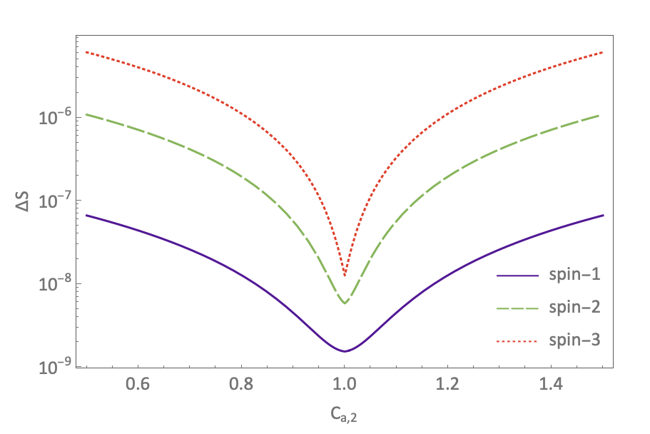
Finally, we expect that including higher spins do not change the main result. The minimum of the relative entropy is always at the Kerr black hole Wilson coefficient point. Moving away from this point quickly increase the entanglement entropy. A comparison between the spin-1, spin-2 and spin-3 cases keeping all Wilson coefficients one except can be seen in fig. 6.


V Conclusions and outlook
In this letter, we consider the entanglement entropy generated by gravitationally coupled binary systems. By considering the Hilbert space of spin states, we demonstrate that minimal coupling for massive arbitrary spin particle have the unique feature of generating nearly zero entanglement in the scattering process. Given the correspondence between minimal coupling and rotating black holes, the result suggests that such feature can also be attributed to the entanglement properties of spinning black holes. Note that such phenomenon is reminiscent of what was found in strong interactions, where entanglement suppression is associated with symmetry enhancement Beane et al. 2019.
While the relative entropy is near zero, it is not zero, which may be an artifact of confining ourselves to leading order in Eikonal approximation. This makes clear investigation at NLO is desirable. As mentioned in the introduction, there is a general correspondence between minimal coupling and black-hole like solutions in four-dimensions. This includes Reissner Nordstrom, Kerr Newman Moynihan 2020; Chung et al. 2019c, Taub-NUT Huang et al. 2019 and Kerr-Taub NUT Emond et al.. Furthermore, gravitationally induced spin-multipoles has also been studied recently in the context of fuzzball microstates Bena and Mayerson 2020a; Bena and Mayerson 2020b; Bianchi et al. 2020. For Kerr Newman there are additional electromagnetic spin multipoles, while for Kerr-Taub NUT and fuzzballs, the minimal couplings are dressed with additional complex phase factors. It will be fascinating to explore their features through the prism of spin entanglement. Finally, it will also be interesting to understand quantum corrections, in particular whether or not they generate anomalous gravitational multipole moments.
Acknowledgements
We would especially like to thank Jung-Wook Kim, for discussions on the computation of Eikonal phase for spin effects. Also Bo-Ting Chen, Tzu-Chen Huang, Jun-Yu Liu and Andreas Helset for enlightening discussions. C.S.M. thanks Hugo Marrochio for the encouragement in the early stages of the project. The work of C.S.M. and R.A. is supported by the Alexander von Humboldt Foundation, in the framework of the Sofja Kovalevskaja Award 2016, endowed by the German Federal Ministry of Education and Research and also supported by the Cluster of Excellence “Precision Physics, Fundamental Interactions, and Structure of Matter” (PRISMA+ EXC 2118/1) funded by the German Research Foundation (DFG) within the German Excellence Strategy (Project ID 39083149). Mz C, Yt H, and Mk T is supported by MoST Grant No. 106-2628-M-002-012-MY3. Yt H is also supported by Golden Jade fellowship.
References
- Arkani-Hamed et al. (2017) N. Arkani-Hamed, T.-C. Huang, and Y.-t. Huang, Scattering Amplitudes For All Masses and Spins, (2017), arXiv:1709.04891 [hep-th].
- Guevara (2019) A. Guevara, Holomorphic Classical Limit for Spin Effects in Gravitational and Electromagnetic Scattering, JHEP 04 (2019) 033, arXiv:1706.02314 [hep-th].
- Chung et al. (2019a) M.-Z. Chung, Y.-T. Huang, J.-W. Kim, and S. Lee, The simplest massive S-matrix: from minimal coupling to Black Holes, JHEP 04 (2019a) 156, arXiv:1812.08752 [hep-th].
- Guevara et al. (2019) A. Guevara, A. Ochirov, and J. Vines, Scattering of Spinning Black Holes from Exponentiated Soft Factors, JHEP 09 (2019) 056, arXiv:1812.06895 [hep-th].
- Arkani-Hamed et al. (2020) N. Arkani-Hamed, Y.-t. Huang, and D. O’Connell, Kerr black holes as elementary particles, JHEP 01 (2020) 046, arXiv:1906.10100 [hep-th].
- Aoude et al. (2020) R. Aoude, K. Haddad, and A. Helset, On-shell heavy particle effective theories, JHEP 05 (2020) 051, arXiv:2001.09164 [hep-th].
- Goldberger and Rothstein (2006) W. D. Goldberger and I. Z. Rothstein, An Effective field theory of gravity for extended objects, Phys. Rev. D73 (2006) 104029, arXiv:hep-th/0409156.
- Porto and Rothstein (2008) R. A. Porto and I. Z. Rothstein, Spin(1)Spin(2) Effects in the Motion of Inspiralling Compact Binaries at Third Order in the Post-Newtonian Expansion, Phys. Rev. D78 (2008) 044012, [Erratum: Phys. Rev.D81,029904(2010)], arXiv:0802.0720 [gr-qc].
- Cervera-Lierta et al. (2017) A. Cervera-Lierta, J. I. Latorre, J. Rojo, and L. Rottoli, Maximal Entanglement in High Energy Physics, SciPost Phys. 3 (2017) 036, arXiv:1703.02989 [hep-th].
- Beane et al. (2019) S. R. Beane, D. B. Kaplan, N. Klco, and M. J. Savage, Entanglement Suppression and Emergent Symmetries of Strong Interactions, Phys. Rev. Lett. 122 (2019) 102001, arXiv:1812.03138 [nucl-th].
- Afik and de Nova (2020) Y. Afik and J. de Nova, Enanglement detection at the LHC, (2020), arXiv:2003.02280 [quant-ph].
- Bose et al. (2020) A. Bose, P. Haldar, A. Sinha, P. Sinha, and S. S. Tiwari, Relative entropy in scattering and the S-matrix bootstrap, (2020), arXiv:2006.12213 [hep-th].
- Peschanski and Seki (2016) R. Peschanski and S. Seki, Entanglement Entropy of Scattering Particles, Phys. Lett. B 758 (2016) 89, arXiv:1602.00720 [hep-th].
- Peschanski and Seki (2019) R. Peschanski and S. Seki, Evaluation of Entanglement Entropy in High Energy Elastic Scattering, Phys. Rev. D 100 (2019) 076012, arXiv:1906.09696 [hep-th].
- Peres et al. (2002) A. Peres, P. F. Scudo, and D. R. Terno, Quantum entropy and special relativity, Phys. Rev. Lett. 88 (2002) 230402.
- Lindner et al. (2003) N. H. Lindner, A. Peres, and D. R. Terno, Wigner’s little group and Berry’s phase for massless particles, J. Phys. A36 (2003) L449, arXiv:hep-th/0304017.
- He et al. (2008) S. He, S.-x. Shao, and H.-b. Zhang, Entanglement Entropy: Helicity versus Spin, Int. J. Quant. Inf. 6 (2008) 181, arXiv:quant-ph/0702028.
- Chung et al. (2019b) M.-Z. Chung, Y.-T. Huang, and J.-W. Kim, Classical potential for general spinning bodies, (2019b), arXiv:1908.08463 [hep-th].
- Chung et al. (2020) M.-Z. Chung, Y.-t. Huang, J.-W. Kim, and S. Lee, Complete Hamiltonian for spinning binary systems at first post-Minkowskian order, JHEP 05 (2020) 105, arXiv:2003.06600 [hep-th].
- Bern et al. (2020) Z. Bern, A. Luna, R. Roiban, C.-H. Shen, and M. Zeng, Spinning Black Hole Binary Dynamics, Scattering Amplitudes and Effective Field Theory, (2020), arXiv:2005.03071 [hep-th].
- (21) Note that the Lorentz invariance of the entanglement entropy after the inclusion of the Thomas-Wigner rotation factors was also recently demonstrated for -channel fermion-fermion scattering Fan and Li 2018, .
- Nielsen and Chuang (2010) M. A. Nielsen and I. L. Chuang, Quantum Computation and Quantum Information: 10th Anniversary Edition (Cambridge University Press, 2010).
- Levi and Steinhoff (2015) M. Levi and J. Steinhoff, Spinning gravitating objects in the effective field theory in the post-Newtonian scheme, JHEP 09 (2015) 219, arXiv:1501.04956 [gr-qc].
- Maybee et al. (2019) B. Maybee, D. O’Connell, and J. Vines, Observables and amplitudes for spinning particles and black holes, JHEP 12 (2019) 156, arXiv:1906.09260 [hep-th].
- Moynihan (2020) N. Moynihan, Kerr-Newman from Minimal Coupling, JHEP 01 (2020) 014, arXiv:1909.05217 [hep-th].
- Chung et al. (2019c) M.-Z. Chung, Y.-T. Huang, and J.-W. Kim, Kerr-Newman stress-tensor from minimal coupling to all orders in spin, (2019c), arXiv:1911.12775 [hep-th].
- Huang et al. (2019) Y.-T. Huang, U. Kol, and D. O’Connell, The Double Copy of Electric-Magnetic Duality, (2019), arXiv:1911.06318 [hep-th].
- (28) W. Emond, Y.-T. Huang, U. Kol, N. Moynihan, and D. O’Connell, In peperation, .
- Bena and Mayerson (2020a) I. Bena and D. R. Mayerson, A New Window into Black Holes, (2020a), arXiv:2006.10750 [hep-th].
- Bena and Mayerson (2020b) I. Bena and D. R. Mayerson, Black Holes Lessons from Multipole Ratios, (2020b), arXiv:2007.09152 [hep-th].
- Bianchi et al. (2020) M. Bianchi, D. Consoli, A. Grillo, J. F. Morales, P. Pani, and G. Raposo, Distinguishing fuzzballs from black holes through their multipolar structure, (2020), arXiv:2007.01743 [hep-th].
- Fan and Li (2018) J. Fan and X. Li, Relativistic effect of entanglement in fermion-fermion scattering, Phys. Rev. D 97 (2018) 016011, arXiv:1712.06237 [hep-th].
- Kim (2020) J.-W. Kim, Quantum point particle approximation of spinning black holes and compact stars, Other thesis (2020), arXiv:2007.12398 [hep-th].
Supplemental Material
VI Little group spin operators
Since the spin vector appearing in the eikonal phase is the little group spin operator , we work out its components here by plugging in explicit parametrizations of all the variables. We parameterize the momentum as
| (17) |
where the corresponding spinors are given byKim 2020
| (18) |
with the ket vectors being the eigenvectors of :
| (19) |
Spin
The little group spin operator is
| (20) |
with and being the chiral and anti-chiral part of the Pauli-Lubasnki operator. Plugging in the explicit form of the spinors in eq.(18), one would get
| (21) |
which matches with the first line of eq.(2.17) in Bern et al. 2020 when we set their .
Spin 1
For spin 1, the little group spin operator is given by
| (22) |
where is the massive spin 1 polarization vector and . It relates to the spinor helicity variables by:
| (23) |
Plugging the parametrization given by eq.(18) into the above equation, we would get
| (24) |
where
| (25) |
We see again that our little group operator matches the first line of eq.(2.17) in Bern et al. 2020 when .
VII Fourier transforming into impact parameter space
| (26) | ||||
VIII Data and More Plots
Here we show the plots for setting and scan through different combinations of and to show minimal increment of entropy in a binary black hole system is robust.


Finally we give the data for Fig 4. The red highlight corresponds to , where we can see is indeed the minimum.
| -5. | -5. | 1.08 | -2.5 | -2.5 | 0.807 | 0 | 0 | 0.282 | 2.5 | 2.5 | 0.607 |
| -5. | -4.5 | 0.976 | -2.5 | -2. | 0.843 | 0 | 0.5 | 0.102 | 2.5 | 3. | 0.740 |
| -5. | -4. | 1.09 | -2.5 | -1.5 | 0.747 | 0 | 1. | 0.0000219 | 2.5 | 3.5 | 0.793 |
| -5. | -3.5 | 0.869 | -2.5 | -1. | 0.820 | 0 | 1.5 | 0.103 | 2.5 | 4. | 0.791 |
| -5. | -3. | 0.888 | -2.5 | -0.5 | 0.931 | 0 | 2. | 0.282 | 2.5 | 4.5 | 0.851 |
| -5. | -2.5 | 0.823 | -2.5 | 0 | 0.820 | 0 | 2.5 | 0.462 | 2.5 | 5. | 0.941 |
| -5. | -2. | 0.989 | -2.5 | 0.5 | 0.469 | 0 | 3. | 0.608 | 3. | -5. | 1.15 |
| -5. | -1.5 | 0.901 | -2.5 | 1. | 0.000184 | 0 | 3.5 | 0.714 | 3. | -4.5 | 1.08 |
| -5. | -1. | 0.893 | -2.5 | 1.5 | 0.427 | 0 | 4. | 0.790 | 3. | -4. | 1.01 |
| -5. | -0.5 | 0.796 | -2.5 | 2. | 0.758 | 0 | 4.5 | 0.835 | 3. | -3.5 | 1.03 |
| -5. | 0 | 0.802 | -2.5 | 2.5 | 0.815 | 0 | 5. | 0.847 | 3. | -3. | 1.06 |
| -5. | 0.5 | 0.582 | -2.5 | 3. | 0.992 | 0.5 | -5. | 0.582 | 3. | -2.5 | 0.992 |
| -5. | 1. | 0.000297 | -2.5 | 3.5 | 1.03 | 0.5 | -4.5 | 0.574 | 3. | -2. | 0.883 |
| -5. | 1.5 | 0.485 | -2.5 | 4. | 1.03 | 0.5 | -4. | 0.560 | 3. | -1.5 | 0.854 |
| -5. | 2. | 0.783 | -2.5 | 4.5 | 1.13 | 0.5 | -3.5 | 0.539 | 3. | -1. | 0.877 |
| -5. | 2.5 | 0.963 | -2.5 | 5. | 1.13 | 0.5 | -3. | 0.510 | 3. | -0.5 | 0.802 |
| -5. | 3. | 1.15 | -2. | -5. | 0.989 | 0.5 | -2.5 | 0.469 | 3. | 0 | 0.608 |
| -5. | 3.5 | 1.15 | -2. | -4.5 | 0.972 | 0.5 | -2. | 0.415 | 3. | 0.5 | 0.273 |
| -5. | 4. | 1.12 | -2. | -4. | 0.905 | 0.5 | -1.5 | 0.347 | 3. | 1. | 0.0000760 |
| -5. | 4.5 | 1.13 | -2. | -3.5 | 0.820 | 0.5 | -1. | 0.269 | 3. | 1.5 | 0.258 |
| -5. | 5. | 1.03 | -2. | -3. | 0.830 | 0.5 | -0.5 | 0.185 | 3. | 2. | 0.546 |
| -4.5 | -5. | 0.976 | -2. | -2.5 | 0.843 | 0.5 | 0 | 0.102 | 3. | 2.5 | 0.740 |
| -4.5 | -4.5 | 1.08 | -2. | -2. | 0.745 | 0.5 | 0.5 | 0.0338 | 3. | 3. | 0.801 |
| -4.5 | -4. | 0.922 | -2. | -1.5 | 0.785 | 0.5 | 1. | 6.08 | 3. | 3.5 | 0.835 |
| -4.5 | -3.5 | 0.842 | -2. | -1. | 0.900 | 0.5 | 1.5 | 0.0339 | 3. | 4. | 0.958 |
| -4.5 | -3. | 0.782 | -2. | -0.5 | 0.917 | 0.5 | 2. | 0.103 | 3. | 4.5 | 1.08 |
| -4.5 | -2.5 | 0.955 | -2. | 0 | 0.769 | 0.5 | 2.5 | 0.187 | 3. | 5. | 1.17 |
| -4.5 | -2. | 0.972 | -2. | 0.5 | 0.415 | 0.5 | 3. | 0.273 | 3.5 | -5. | 1.15 |
| -4.5 | -1.5 | 0.828 | -2. | 1. | 0.000147 | 0.5 | 3.5 | 0.354 | 3.5 | -4.5 | 1.15 |
| -4.5 | -1. | 0.901 | -2. | 1.5 | 0.388 | 0.5 | 4. | 0.424 | 3.5 | -4. | 1.16 |
| -4.5 | -0.5 | 0.782 | -2. | 2. | 0.726 | 0.5 | 4.5 | 0.482 | 3.5 | -3.5 | 1.11 |
| -4.5 | 0 | 0.833 | -2. | 2.5 | 0.830 | 0.5 | 5. | 0.526 | 3.5 | -3. | 1.02 |
| -4.5 | 0.5 | 0.574 | -2. | 3. | 0.883 | 1. | -5. | 0.000297 | 3.5 | -2.5 | 1.03 |
| -4.5 | 1. | 0.000288 | -2. | 3.5 | 1.03 | 1. | -4.5 | 0.000288 | 3.5 | -2. | 1.03 |
| -4.5 | 1.5 | 0.486 | -2. | 4. | 1.01 | 1. | -4. | 0.000272 | 3.5 | -1.5 | 0.912 |
| -4.5 | 2. | 0.749 | -2. | 4.5 | 1.01 | 1. | -3.5 | 0.000248 | 3.5 | -1. | 0.875 |
| -4.5 | 2.5 | 1.00 | -2. | 5. | 1.11 | 1. | -3. | 0.000219 | 3.5 | -0.5 | 0.876 |
| -4.5 | 3. | 1.08 | -1.5 | -5. | 0.901 | 1. | -2.5 | 0.000184 | 3.5 | 0 | 0.714 |
| -4.5 | 3.5 | 1.15 | -1.5 | -4.5 | 0.828 | 1. | -2. | 0.000147 | 3.5 | 0.5 | 0.354 |
| -4.5 | 4. | 1.13 | -1.5 | -4. | 0.839 | 1. | -1.5 | 0.000111 | 3.5 | 1. | 0.000111 |
| -4.5 | 4.5 | 1.16 | -1.5 | -3.5 | 0.881 | 1. | -1. | 0.0000759 | 3.5 | 1.5 | 0.325 |
| -4.5 | 5. | 1.09 | -1.5 | -3. | 0.824 | 1. | -0.5 | 0.0000458 | 3.5 | 2. | 0.634 |
| -4. | -5. | 1.09 | -1.5 | -2.5 | 0.747 | 1. | 0 | 0.0000219 | 3.5 | 2.5 | 0.793 |
| -4. | -4.5 | 0.922 | -1.5 | -2. | 0.785 | 1. | 0.5 | 6.08 | 3.5 | 3. | 0.835 |
| -4. | -4. | 0.835 | -1.5 | -1.5 | 0.882 | 1. | 1. | 1.26 | 3.5 | 3.5 | 0.993 |
| -4. | -3.5 | 0.804 | -1.5 | -1. | 0.942 | 1. | 1.5 | 6.08 | 3.5 | 4. | 1.15 |
| -4. | -3. | 0.908 | -1.5 | -0.5 | 0.874 | 1. | 2. | 0.0000219 | 3.5 | 4.5 | 1.17 |
| -4. | -2.5 | 1.01 | -1.5 | 0 | 0.701 | 1. | 2.5 | 0.0000458 | 3.5 | 5. | 1.13 |
| -4. | -2. | 0.905 | -1.5 | 0.5 | 0.347 | 1. | 3. | 0.0000760 | 4. | -5. | 1.12 |
| -4. | -1.5 | 0.839 | -1.5 | 1. | 0.000111 | 1. | 3.5 | 0.000111 | 4. | -4.5 | 1.13 |
| -4. | -1. | 0.835 | -1.5 | 1.5 | 0.333 | 1. | 4. | 0.000148 | 4. | -4. | 1.16 |
| -4. | -0.5 | 0.787 | -1.5 | 2. | 0.665 | 1. | 4.5 | 0.000185 | 4. | -3.5 | 1.15 |
| -4. | 0 | 0.867 | -1.5 | 2.5 | 0.846 | 1. | 5. | 0.000219 | 4. | -3. | 1.14 |
| -4. | 0.5 | 0.560 | -1.5 | 3. | 0.854 | 1.5 | -5. | 0.485 | 4. | -2.5 | 1.03 |
| -4. | 1. | 0.000272 | -1.5 | 3.5 | 0.912 | 1.5 | -4.5 | 0.486 | 4. | -2. | 1.01 |
| -4. | 1.5 | 0.482 | -1.5 | 4. | 1.01 | 1.5 | -4. | 0.482 | 4. | -1.5 | 1.01 |
| -4. | 2. | 0.727 | -1.5 | 4.5 | 1.00 | 1.5 | -3.5 | 0.471 | 4. | -1. | 0.901 |
| -4. | 2.5 | 1.01 | -1.5 | 5. | 0.979 | 1.5 | -3. | 0.453 | 4. | -0.5 | 0.882 |
| -4. | 3. | 1.01 | -1. | -5. | 0.893 | 1.5 | -2.5 | 0.427 | 4. | 0 | 0.790 |
| -4. | 3.5 | 1.16 | -1. | -4.5 | 0.901 | 1.5 | -2. | 0.388 | 4. | 0.5 | 0.424 |
| -4. | 4. | 1.16 | -1. | -4. | 0.835 | 1.5 | -1.5 | 0.333 | 4. | 1. | 0.000148 |
| -4. | 4.5 | 1.07 | -1. | -3.5 | 0.770 | 1.5 | -1. | 0.264 | 4. | 1.5 | 0.377 |
| -4. | 5. | 1.17 | -1. | -3. | 0.772 | 1.5 | -0.5 | 0.184 | 4. | 2. | 0.704 |
| -3.5 | -5. | 0.869 | -1. | -2.5 | 0.820 | 1.5 | 0 | 0.103 | 4. | 2.5 | 0.791 |
| -3.5 | -4.5 | 0.842 | -1. | -2. | 0.900 | 1.5 | 0.5 | 0.0339 | 4. | 3. | 0.958 |
| -3.5 | -4. | 0.804 | -1. | -1.5 | 0.942 | 1.5 | 1. | 6.08 | 4. | 3.5 | 1.15 |
| -3.5 | -3.5 | 0.912 | -1. | -1. | 0.896 | 1.5 | 1.5 | 0.0337 | 4. | 4. | 1.16 |
| -3.5 | -3. | 1.06 | -1. | -0.5 | 0.794 | 1.5 | 2. | 0.101 | 4. | 4.5 | 1.18 |
| -3.5 | -2.5 | 0.993 | -1. | 0 | 0.604 | 1.5 | 2.5 | 0.181 | 4. | 5. | 1.18 |
| -3.5 | -2. | 0.820 | -1. | 0.5 | 0.269 | 1.5 | 3. | 0.258 | 4.5 | -5. | 1.13 |
| -3.5 | -1.5 | 0.881 | -1. | 1. | 0.0000759 | 1.5 | 3.5 | 0.325 | 4.5 | -4.5 | 1.16 |
| -3.5 | -1. | 0.770 | -1. | 1.5 | 0.264 | 1.5 | 4. | 0.377 | 4.5 | -4. | 1.07 |
| -3.5 | -0.5 | 0.824 | -1. | 2. | 0.580 | 1.5 | 4.5 | 0.417 | 4.5 | -3.5 | 1.18 |
| -3.5 | 0 | 0.875 | -1. | 2.5 | 0.785 | 1.5 | 5. | 0.446 | 4.5 | -3. | 1.14 |
| -3.5 | 0.5 | 0.539 | -1. | 3. | 0.877 | 2. | -5. | 0.783 | 4.5 | -2.5 | 1.13 |
| -3.5 | 1. | 0.000248 | -1. | 3.5 | 0.875 | 2. | -4.5 | 0.749 | 4.5 | -2. | 1.01 |
| -3.5 | 1.5 | 0.471 | -1. | 4. | 0.901 | 2. | -4. | 0.727 | 4.5 | -1.5 | 1.00 |
| -3.5 | 2. | 0.733 | -1. | 4.5 | 0.954 | 2. | -3.5 | 0.733 | 4.5 | -1. | 0.954 |
| -3.5 | 2.5 | 0.949 | -1. | 5. | 0.986 | 2. | -3. | 0.754 | 4.5 | -0.5 | 0.889 |
| -3.5 | 3. | 1.03 | -0.5 | -5. | 0.796 | 2. | -2.5 | 0.758 | 4.5 | 0 | 0.835 |
| -3.5 | 3.5 | 1.11 | -0.5 | -4.5 | 0.782 | 2. | -2. | 0.726 | 4.5 | 0.5 | 0.482 |
| -3.5 | 4. | 1.15 | -0.5 | -4. | 0.787 | 2. | -1.5 | 0.665 | 4.5 | 1. | 0.000185 |
| -3.5 | 4.5 | 1.18 | -0.5 | -3.5 | 0.824 | 2. | -1. | 0.580 | 4.5 | 1.5 | 0.417 |
| -3.5 | 5. | 1.07 | -0.5 | -3. | 0.877 | 2. | -0.5 | 0.453 | 4.5 | 2. | 0.736 |
| -3. | -5. | 0.888 | -0.5 | -2.5 | 0.931 | 2. | 0 | 0.282 | 4.5 | 2.5 | 0.851 |
| -3. | -4.5 | 0.782 | -0.5 | -2. | 0.917 | 2. | 0.5 | 0.103 | 4.5 | 3. | 1.08 |
| -3. | -4. | 0.908 | -0.5 | -1.5 | 0.874 | 2. | 1. | 0.0000219 | 4.5 | 3.5 | 1.17 |
| -3. | -3.5 | 1.06 | -0.5 | -1. | 0.794 | 2. | 1.5 | 0.101 | 4.5 | 4. | 1.18 |
| -3. | -3. | 1.02 | -0.5 | -0.5 | 0.670 | 2. | 2. | 0.272 | 4.5 | 4.5 | 1.19 |
| -3. | -2.5 | 0.841 | -0.5 | 0 | 0.461 | 2. | 2.5 | 0.429 | 4.5 | 5. | 1.25 |
| -3. | -2. | 0.830 | -0.5 | 0.5 | 0.185 | 2. | 3. | 0.546 | 5. | -5. | 1.03 |
| -3. | -1.5 | 0.824 | -0.5 | 1. | 0.0000458 | 2. | 3.5 | 0.634 | 5. | -4.5 | 1.09 |
| -3. | -1. | 0.772 | -0.5 | 1.5 | 0.184 | 2. | 4. | 0.704 | 5. | -4. | 1.17 |
| -3. | -0.5 | 0.877 | -0.5 | 2. | 0.453 | 2. | 4.5 | 0.736 | 5. | -3.5 | 1.07 |
| -3. | 0 | 0.856 | -0.5 | 2.5 | 0.661 | 2. | 5. | 0.737 | 5. | -3. | 1.18 |
| -3. | 0.5 | 0.510 | -0.5 | 3. | 0.802 | 2.5 | -5. | 0.963 | 5. | -2.5 | 1.13 |
| -3. | 1. | 0.000219 | -0.5 | 3.5 | 0.876 | 2.5 | -4.5 | 1.00 | 5. | -2. | 1.11 |
| -3. | 1.5 | 0.453 | -0.5 | 4. | 0.882 | 2.5 | -4. | 1.01 | 5. | -1.5 | 0.979 |
| -3. | 2. | 0.754 | -0.5 | 4.5 | 0.889 | 2.5 | -3.5 | 0.949 | 5. | -1. | 0.986 |
| -3. | 2.5 | 0.863 | -0.5 | 5. | 0.899 | 2.5 | -3. | 0.863 | 5. | -0.5 | 0.899 |
| -3. | 3. | 1.06 | 0 | -5. | 0.802 | 2.5 | -2.5 | 0.815 | 5. | 0 | 0.847 |
| -3. | 3.5 | 1.02 | 0 | -4.5 | 0.833 | 2.5 | -2. | 0.830 | 5. | 0.5 | 0.526 |
| -3. | 4. | 1.14 | 0 | -4. | 0.867 | 2.5 | -1.5 | 0.846 | 5. | 1. | 0.000219 |
| -3. | 4.5 | 1.14 | 0 | -3.5 | 0.875 | 2.5 | -1. | 0.785 | 5. | 1.5 | 0.446 |
| -3. | 5. | 1.18 | 0 | -3. | 0.856 | 2.5 | -0.5 | 0.661 | 5. | 2. | 0.737 |
| -2.5 | -5. | 0.823 | 0 | -2.5 | 0.820 | 2.5 | 0 | 0.462 | 5. | 2.5 | 0.941 |
| -2.5 | -4.5 | 0.955 | 0 | -2. | 0.769 | 2.5 | 0.5 | 0.187 | 5. | 3. | 1.17 |
| -2.5 | -4. | 1.01 | 0 | -1.5 | 0.701 | 2.5 | 1. | 0.0000458 | 5. | 3.5 | 1.13 |
| -2.5 | -3.5 | 0.993 | 0 | -1. | 0.604 | 2.5 | 1.5 | 0.181 | 5. | 4. | 1.18 |
| -2.5 | -3. | 0.841 | 0 | -0.5 | 0.461 | 2.5 | 2. | 0.429 | 5. | 4.5 | 1.25 |