Perpetual American options with asset-dependent discountingThanks: Jonas Al-Hadad and Zbigniew Palmowski have been partially supported by the National Science Centre under the grant 2016/23/B/HS4/00566.
Abstract.
In this paper we consider the following optimal stopping problem
where the process is a jump-diffusion process, is a family of stopping times while and are fixed payoff function and discount function, respectively. In a financial market context, if or and is the expectation taken with respect to a martingale measure, describes the price of a perpetual American option with a discount rate depending on the value of the asset process . If is a constant, the above problem produces the standard case of pricing perpetual American options. In the first part of this paper we find sufficient conditions for the convexity of the value function . This allows us to determine the stopping region as a certain interval and hence we are able to identify the form of . We also prove a put-call symmetry for American options with asset-dependent discounting. In the case when is a geometric Lévy process we give exact expressions using the so-called omega scale functions introduced in [54]. We prove that the analysed value function satisfies the HJB equation and we give sufficient conditions for the smooth fit property as well. Finally, we present a few examples for which we obtain the analytical form of the value function .
Keywords. American option Lévy process diffusion Black-Scholes market optimal stopping problem convexity
2010 Mathematics Subject Classification
Primary: 60G40; Secondary: 60J60; 91B281. Introduction
In this paper the uncertainty associated with the stock price is described by a jump-diffusion process defined on a complete filtered risk-neutral probability space , where is a natural filtration of satisfying the usual conditions and is a risk-neutral measure under which the discounted (with respect to a risk-free interest rate) asset price process is a local martingale. We point out that, as noted in [26], introducing jumps into the model, implies lost of completeness of the market which results in the lack of uniqueness of the equivalent martingale measure. Our main goal is the analysis of the following optimal stopping problem
| (1) |
where is a family of -stopping times while and are fixed payoff function and discount function, respectively. Above denotes the expectation with respect to when . We assume that the function is convex. We allow in this paper for to have negative values as well. In the case when or and is a martingale measure, this function can be interpreted as the value function of a perpetual American option with asset-dependent discounting 11 1 Throughout the paper, we use the terms asset-dependent discounting and functional discounting interchangeably. and payoff function . In the case of the general theory of stochastic processes, multiplying by the discount factor corresponds to killing of a generator of by potential .
This problem extends the classical theory of option pricing, where the deterministic discount rate is considered, that is if , then we obtain the standard form
of the perpetual American option’s value function with constant discount rate .
The main objective of this paper is to find a closed expression of (1) and identify the optimal stopping rule for which the supremum is attained. To do this, we start from proving in Theorem 2 an inheritance of convexity property from the payoff function to the value function. This corresponds to preserving the convexity by the solution to a certain obstacle problem.
Using this observation and the classical optimal stopping theory presented e.g. in [63] one can identify the optimal stopping region as an interval , that is, . Hence, in general, one can obtain in this case a double continuation region.
Later we focus on the case when is a geometric spectrally negative Lévy process, that is,
for a spectrally negative Lévy process . In this case, using the fluctuation theory of Lévy processes, we identify the value function (1) in terms of the omega scale functions introduced in [54].
For optimal stopping problem (1) we give sufficient conditions under which we can formalise the classical approach here as well. In particular, in Theorem 9 we prove that if the value function is smooth enough then it is the unique solution to a certain Hamiltonian-Jacobi-Bellman (HJB) system. Moreover, in the case of geometric Lévy process of the asset price , we prove that the regularity of for and ) gives the smooth fit property at the ends of the stopping region. We want to underline here that proving the above mentioned regularity of the value function in the case of the jump-diffusion processes (which allows to formulate the HJB equation) in general is very difficult task (see [3] for some deep results related with it). Nevertheless, it is possible in our case thanks to Theorem 9 and Remark 10. Having the convexity of the value function proved and hence having the value function defined in terms of the omega scale functions, we can prove the appropriate smoothness condition using the fluctuation theory of Lévy processes. Only then one can apply the HJB equation.
Further, even solving the HJB equation does not give in the straightforward way the form of the the stopping region (except, of course, the fact that it is the set where the value function equals the payoff function). This is the reason why we do not follow this path, but rely on our approach allowing us to define precisely the stopping region.
In Theorem 11 we show the put-call symmetry which holds in our setting as well.
These theoretical results allow us to find the price of the perpetual American option with asset-dependent discounting for some particular cases. We take for example a put option, that is , and a geometric Brownian motion for the asset price . We model also by the geometric Lévy process with exponentially distributed downward jumps. We analyse various discount functions . In Section 3 we provide a few examples for which we obtain the analytical form of the value function.
The discount rate changing in time or a random discount rate are widely used in pricing derivatives in financial markets. They have proved to be valuable and flexible tools to identify the value of various options. Usually, either the interest rate is independent from the asset price or this dependence is introduced via taking a correlation between gaussian components of these two processes. Our aim is completely different. We want to understand an extreme case when we have strong, functional dependence between the interest rate and the asset price. In particular, we take a close look at the American put option with the discount function having the opposite monotonicity to the payoff function. At first sight, such a case seems to be counter-intuitive, because, for the put option, if the asset price is in higher region one can expect that the interest rate will be lower and the opposite effect one expects for smaller range of asset’s prices. This dependence somehow balances the discounting function with the payoff function. However, we can think of an investor who have a strong confidence in the movement of the asset price and wishes to make an extra profit when he is right and suffers a greater loss when he is wrong. This concept resembles an idea that stands behind barrier options, i.e. if an investor believes that it is unlikely that the asset price will hit a given level, he can add a knock-out provision with the barrier set at the support level, so he can reduce the price of an option. By including the barrier provision, he can eliminate paying for those scenarios he feels are unlikely. In our approach, we work in two ways by reducing the premium thanks to incidents being improbable from the investor’s perspective and increasing it for scenarios that are more likely to happen. Such a description of the analysed option adequately describes a financial instrument tailored to the risky investor. Let us add that for example up-and-out put options analysed by [55] is a particular case of our option.
One can look at optimisation problem (1) from a wider perspective though. The killing by potential has been known widely in physics and other applied sciences. Then (1) can be seen as a certain functional describing gain or energy and the goal is to optimise it by choosing some random stopping time. We focus here on financial applications only and therefore throughout this paper the price is calculated under the martingale measure. It means more formally that there exists a risk-free interest rate such that the discounted price process is a local martingale under . Note that the discount function may equal the risk-free interest rate but in our case usually is different.
For example, in the case of a gold loan (see [24] for the survey related with this financial instrument) a borrower receives at time (the date of contract inception) a loan amount using one mass unit (one troy ounce, say) of gold as collateral, which must be physically delivered to a lender. This amount grows at the functional borrowing rate given in the contract that can depend on the gold spot price . When paying back the loan, the borrower can redeem the gold at any time and then the contract is terminated. Of course, the dynamic of under the risk-neutral measure is such that the discounted price is a martingale, that is . Assume that the costs of storing equals the borrowing rate plus some fixed costs per unit of time and the borrowing rate is a function of the gold spot price discounted by this fixed costs. Then the value of the contract, with infinite maturity date, at time equals
where , and .
Our research methodology is based on combining the theory of partial differential equations with the fluctuation theory of Lévy processes.
To prove the convexity we start from proving in Theorem 20 the convexity of
| (2) |
for fixed time horizon , where is the expectation with respect to when . In the proof we follow the idea given by Ekström and Tysk in [38]. Namely, the value function given in (2) can be presented as the unique viscosity solution to a certain Cauchy problem for some second-order operator related to the generator of the process . In fact, applying similar arguments like in [65, Proposition 5.3] and [38, Lemma 3.1], one can show that, under some additional assumptions, this solution can be treated as the classical one. Then we can formulate the sufficient locally convexity preserving conditions for the infinitesimal preservation of convexity at some point. This characterisation is given in terms of a differential inequality on the coefficients of the considered operator. It also allows to prove the convexity of . Then, in Theorem 2 and Lemma 24 we apply the dynamic programming principle (see [37]) in order to generalise the convexity property of to the value function .
Later we focus on the American put option with the value function
where the payoff function for some strike price . Using the convexity property mentioned above we can conclude that the optimal stopping rule is defined as the first entrance of the process to the interval , that is,
| (3) |
In the next step, one has to identify
| (4) |
and take maximum over levels and to identify the optimal stopping rule and to find the value function . This is done for the geometric spectrally negative Lévy process where is a spectrally negative Lévy process starting at . We recall that spectrally negative Lévy processes do not have positive jumps. Hence, in particular, our analysis could be applied for the Black-Scholes market where is a Brownian motion with a drift. To execute this plan we express in terms of the laws of the first passage times and then we use the fluctuation theory developed in [54]. In the whole analysis the use of the change of measure technique developed in [61] is crucial as well.
Optimal levels and of the stopping region and the price of the American put option could be found by application of the appropriate HJB equation. We prove this HJB equation and the smooth fit condition relying on the classical approach of [52] and [63].
Finally, to find the price of the American call option we prove the put-call symmetry in our set-up. The proof is based on the exponential change of measure introduced in [61].
We analyse in detail the Black-Scholes model and the case when a logarithm of the asset price is a geometric linear drift minus compound Poisson process with exponentially distributed jumps and various discount functions . The first example shows changes of the American options’ prices in a gaussian and continuous market while the latter is to model the market including downward shocks in the assets’ behaviour. In this paper we present some specific examples for these two cases.
Our paper seems to be the first one analysing the optimal problem of the form (1) in this generality for jump-diffusion processes. For the classical diffusion processes Lamberton in [53] proved that the value function in (1) is continuous and can be characterised as the unique solution to a variational inequality in the sense of distributions. Another crucial paper for our considerations is [11] which introduced discounting via a positive continuous additive functional of the process and used the approach of Itô and McKean [43, Sec. 4.6] to characterise the value function. Note that is indeed additive functional. A similar problem was also considered in [56].
If for a strike then which equals the area under the trajectory of . Therefore, in this special case we can talk about the so-called area options; see [28] for details.
Another interesting paper of Rodosthenous and Zhang [66] concerns the optimal stopping of an American call option in a random time-horizon under a geometric spectrally negative Lévy model. The random time-horizon is modeled by an omega default clock which is in their case the first time when the occupation time of the asset price below a fixed level exceeds an independent exponential random variable with mean . This corresponds to the special case of our discounting with , where is a risk-free interest rate.
Similar discounting was analysed in [33, 55] where American step options were considered. In this case where . Moreover, the payoff function of a step option is the same as the payoff of a vanilla option, except that it is deflated by a factor when the knock-out rate is positive or inflated by the same factor when the knock-in rate is negative. In both cases, the factor depends exponentially on the cumulative excursion time above or below a given barrier during the entire life of the option. This exponential functional can be hence interpreted as a knock-out (knock-in) discount factor. Step options are mainly traded over-the-counter. They can serve as a benchmark for the analysis and the design of certain classes of occupation-time derivatives and related structured products.
This idea can be further generalised in a sense that the discount function can be treated in the realm of real options as more general knock-out (knock-in) factor. One of the advantages of this type of the functional discounting is that an option buyer can customize the option by selecting an appropriate functional rate according to his risk aversion and the degree of confidence how the asset price will look like during the whole option’s life. From the risk management perspective we can still hedge this option by trading the underlying asset and we can still identify the value of the contract. Additionally, since different market participants can select different discount rates, short-term manipulation by traders is substantially more difficult and therefore considering such options may help reducing market volatility.
The pricing technique developed in this paper can be applied to a wide range of securities and financial contracts where the discounting in the above vein is affected by the underlying asset price process. Apart from the above mentioned examples of options, one can consider for example Executive Stock Options (EOSs) in which the executive may exercise ESOs prematurely and leave the firm if an interesting opportunity arises or for diversification or liquidity reasons. Hence this policy can be determined by publicly available information such as stock prices. As Carr and Linetsky [19] noted this option corresponds either to or , where is a constant intensity of early exercise or forfeiture due to the exogenous voluntary or involuntary employment termination and is the constant intensity of the early exercise due to the executive’s exogenous desire for liquidity or diversification. Another relevant application concerns R&D projects. Here, the likelihood of achieving success before a competitor can depend on the ability of the firm to invest resources in the discovery process. If performance is poor, for instance due to mismanagement, then the firm does not invest resources in the discovery process. In the opposite scenario, more resources are devoted to research activities. Hence the price of this type of projects depends on the path-depended discounting as well; see [70] for survey.
The convexity of the value function and convexity preserving property, which is a key ingredient of our analysis, have been studied quite extensively, see e.g. [13, 14, 21, 36, 40, 41, 45, 46] for diffusion models, and [39, 44] for one-dimensional jump-diffusion models.
We model dynamic of the asset price in a financial market by the jump-diffusion process. The reason to take into account more general class of stochastic processes of asset prices than in the seminal Black-Scholes market is the empirical observation that the log-prices of stocks have a heavier left tail than the normal distribution, on which the seminal Black-Scholes model is founded. The introduction of jumps in the financial market dates back to [58], who added a compound Poisson process to the standard Brownian motion to better describe dynamic of the logarithm of stocks. Since then, there have been many papers and books working in this set-up, see e.g. [26, 68] and references therein. In particular, [26, Table 1.1, p. 29] gives many other reasons to consider this type of market. Apart from the classical Black-Scholes market one can consider the normal inverse Gaussian model of [60], the hyperbolic model of [34], the variance gamma model of [57], the CGMY model of [18], and the tempered stable process analysed in [15, 48]. American options in the jump-diffusion markets have been studied in many papers as well; see e.g. [1, 2, 4, 9, 15, 20, 22, 47, 59].
Identifying the solution of the optimal stopping problem by solving the corresponding HJB equation (as it is done in this paper as well) has been widely used; see [49, 63] for details. In the context of American options with the constant discount function both methods of variational inequalities and viscosity solutions to the boundary value problems in the spirit of Bensoussan and Lions [12] are also well-known; see e.g. [52, 64, 65].
To determine the unknown boundary of stopping region usually the smooth fit condition is applied; see e.g. [51, 52] for the geometric Lévy process of asset prices. As Lamberton and Mikou [52] and Kyprianou and Surya [51] showed the continuous fit is always satisfied but not necessary the smooth fit property. Therefore we prove that appropriate regularities of the process at critical points mentioned already above give smooth paste conditions which generalises the classical results derived by [52, 51]. What we want to underline here is that using our approach (proving convexity and maximising over ends and of the stopping interval ) allows to avoid identifying critical points via smooth paste conditions.
Apart from this, the interval form of the stopping region (hence producing double-sided continuation region) is much more rare. It might come for example from the fact that when at time the discount rate is negative. Then it is worth to wait since discounting might increase the profit from such option. This phenomenon has been already observed for fixed negative discounting (see [6, 7, 8, 29, 71]) or in the case of American capped options with positive interest rate (see [16, 30]).
In this paper we also prove that in this general setting of asset-dependent discounting, one can express the price of the call option in terms of the price of the put option. It is called the put-call symmetry (or put-call parity). Our finding supplements [35, 42] who extend to the Lévy market the findings by [17]. An analogous result for the negative discount rate case was obtained in [6, 7, 8, 29]. A comprehensive review of the put-call duality for American options is given in [31]. We also refer to [32, Section 7] and other references therein for a general survey on the American options in the jump-diffusion model.
The paper is organised as follows. In Section 2 we introduce basic notations and assumptions that we use throughout the paper and we give the main results of this paper. In Section 3, we present a few examples for which we obtain the analytical form of the value function, i.e. for the Black-Scholes market with negative function and for the market with prices being modeled by geometric Lévy process with zero volatility and downward exponential jumps and being a linear function. Section 4 contains proofs of all relevant theorems. We put into Appendix proofs of auxiliary lemmas. The last section includes our concluding remarks.
2. Main results
2.1. Jump-diffusion process
In this paper we assume a jump-diffusion financial market defined formally as follows. On the basic probability space we define a couple adapted to the filtration , where is a standard Brownian motion and is an independent of homogeneous Poisson random measure on for . Then the stock price process solves the following stochastic differential equation
| (5) |
where
- •
is a compensated jump martingale random measure of ,
- •
is a homogenous Poisson random measure defined on with intensity measure
If additionally, the jump-diffusion process has finite activity of jumps, i.e. when
then is a Poisson process and can be represented as
where are i.i.d. random variables independent of with distribution . Note that and are independent of each other as well. When additionally , and , then the asset price process is the geometric Lévy process, that is,
| (6) |
where is a Lévy process starting at with a triple for
| (7) |
This observation follows straightforward from Itô’s rule.
2.2. Assumptions
Before we present the main results of this paper, we state now the assumptions on the model parameters used later on. We denote . If we talk about convexity and concavity we mean it in a weak sense allowing these functions to be constants within some regions.
Assumptions (A)
- (A1)
The drift parameter : and the diffusion parameter : are continuous functions, while the jump size : is measurable and for each fixed , the function is continuous.
- (A2)
There exists a constant such that
for all .
- (A3)
There exists a constant such that
for all .
- (A4)
There exists a constant such that
for all .
- (A5)
, where denotes the set of functions of at most polynomial growth.
- (A6)
is bounded from below.
2.3. Convexity of the value function
Our first main result concerns the convexity of the value function .
Theorem 2.
The proof of the above theorem is given in Section 4.
Remark 3.
We give now sufficient conditions in terms of model parameters for (9) to be satisfied. If is the geometric Lévy process (hence , and ) then (8) is satisfied. Let additionally . Then our optimal stopping problem is equivalent to pricing the perpetual American put option with functional discounting. If is non-decreasing function then the function is non-increasing. Hence in this case condition (9) is satisfied as well. Concluding, if is concave and non-decreasing, then the value function of the perpetual American put option in geometric Lévy market is convex as a function of the initial asset price .
Remark 4.
We have engineered above assumptions to handle mainly the put option (not a call option). The call option can be then handled via put-call symmetry proved in Theorem 11. Hence there is no need to provide sufficient conditions for both cases.
2.4. American put option and the optimal exercise time
Assume now the particular case of (1) with the payoff function
that is, the value function describes the price of a perpetual American put option. The value function for this special choice of payoff function is denoted by
| (10) |
Note that above we used the fact that the option will not be realised when it equals zero, hence the plus in the payoff function could be skipped.
From [63, Thm. 2.7, p. 40] it follows that the optimal stopping rule is of the form
From Theorem 2 we know that is convex. Moreover, from the definition of the value function it follows that . Having both these facts in mind, together with linearity of the payoff function, it follows that and can cross each other in at most two points. This observation leads straightforward to the conclusion about the form of the stopping region. We recall that in (3) and (4) we introduced the entrance time into the interval and the corresponding value function , respectively.
Theorem 5.
Remark 6.
Another characterisation of critical points and via smooth fit property is given in Theorem 9.
Theorem 5 indicates that the optimal stopping rule in our problem is the first time when the process enters the interval for some . In the case when the interval becomes a point which is possible as well. In some cases the above observation allows to identify the value function in a much more transparent way. Finally, note that if the discount function is nonnegative, then it is never optimal to wait to exercise the option for small asset prices, that is, always and the stopping region is one-sided.
2.5. Spectrally negative geometric Lévy process
We can express the value function explicitly for the spectrally negative geometric Lévy process defined in (6), that is when
where is a spectrally negative Lévy process with and hence . This means that does not have positive jumps which corresponds to the inclusion of the support of Lévy measure on the negative half-line. This is very common assumption which is justified by some financial crashes; see e.g. [2, 5, 20]. One can easily observe that the dual case of spectrally positive Lévy process can be also handled in a similar way. We decided to skip this analysis and focus only on a more natural, from a practical perspective, spectrally negative scenario. We express the value function in terms of some special functions, called omega scale functions; see [54] for details.
To introduce these functions let us define first the Laplace exponent via
which is finite al least for due to downward jumps. This function is strictly convex, differentiable, equals zero at zero and tends to infinity at infinity. Hence there exists its right inverse for .
The key functions for the fluctuation theory are the scale functions; see [25]. The first scale function is the unique right continuous function disappearing on the negative half-line whose Laplace transform is
| (11) |
for .
For any measurable function we define the -scale functions , and as the unique solutions to the following renewal-type equations
| (12) | ||||
| (13) | ||||
| (14) |
where is a classical zero scale function and in equation (14) it is additionally assumed that for all and some constant . We also define the function solving the following equation
| (15) |
We introduce the following counterparts of the scale functions (12), (13), (14) and (15)
| (16) | ||||
| (17) | ||||
| (18) | ||||
| (19) |
where .
For for which the Laplace exponent is well-defined we can define a new probability measure via
| (20) |
By [61] and [50, Cor. 3.10], under , the process is again spectrally negative Lévy process with the Laplace exponent of the form
| (21) |
For this new probability measure we can define -scale functions which are denoted by adding subscript to the regular counterparts, hence we have , , and .
We additionally define the following functions
The main result is given in terms of the resolvent density at of starting at killed by the potential and on exiting from positive half-line given by
| (22) |
where
Theorem 7.
The proof of the above theorem is given in Section 4.
2.6. HJB, smooth and continuous fit properties
The classical approach via HJB system is possible in our set-up as well. More precisely, as before in (6) we have
for the Lévy process with the triple (. We start from the observation that using [67, Thm. 31.5, Chap. 6] and Itô’s formula one can conclude that the process is a Markov process with an infinitesimal generator
where is the linear second-order differential operator of the form
and is the integral operator given by
The domain of this generator consists of the functions belonging to if and if . In this paper we prove that satisfies the HJB equation given below with appropriate smooth fit conditions. We recall that is regular for and for the process if for . Similarly, we can define regularity for . Note that regularity of at corresponds to regularity of at for the negative or positive half-line.
Theorem 9.
Let be a bounded from below and concave function with the opposite monotonicity to the payoff function . Assume that and . Then solves uniquely the following HJB system
| (24) |
Moreover, if is regular for and for the process then there is a smooth fit at the right end of the stopping region
Similarly, if is regular for and for the process then there is a smooth fit at the left end of the stopping region
The proof of the above theorem is given in Section 4.
Remark 10.
Let us consider the American put option. Then from Theorems 5 and 7, we can conclude that smoothness of the value function corresponds to the smoothness of the -scale functions for , and . From the definition of these functions given in (12), (13) and (14) it follows that the smoothness of the latter functions is equivalent to the smoothness of the first scale function observed under measures and . By [50, Lem. 8.4] the smoothness of the first scale function does not change under the exponential change of measure (20). Thus from [25, Lem. 2.4, Thms 3.10 and 3.11] if follows that
- •
if then ;
- •
if and the jump measure is absolutely continuous or , then .
Moreover, by [2, Prop. 7], is regular for both and if . Hence HJB system (24) with the smooth fit property could be used without any additional assumptions as long as . If one has single continuation region and then by [2, Prop. 7] to get the smooth fit condition at it is sufficient to assume that the drift of the process is strictly negative.
2.7. Put-call symmetry
The put-call parity allows to calculate the American call option price having the put one. We formulate this relation again for being a general geometric Lévy process defined in (6), that is, for being a general spectrally negative Lévy process having triple
for and defined in (7) and starting position . Apart from the function
defined in (4) we denote
Theorem 11.
Assume that is finite. Let . Then we have
| (25) |
where
| (26) | ||||
Moreover, if assumptions of Theorem 2 hold for the function then the American call option admits a double continuation region with optimal stopping boundaries and such that
| (27) |
where and are the stopping boundaries for the put option.
The proof of the above theorem is given in Section 4.
Remark 12.
Note that the value function of the American call option is expressed in terms of the American put option calculated for the Lévy process being dual to process observed under the measure . In particular, the jumps of the process have the opposite direction to the jumps of the process for which the put option is priced. In general, determining the conditions for such that satisfies all the assumptions of Theorem 2 seems to be impossible and then we can only work on a case-by-case basis.
2.8. Black-Scholes model
We can give more detailed analysis in the case of Black–Scholes model in which the stock price process , where
| (28) |
with , while and are the parameters called drift and volatility, respectively. Under the martingale measure we have , where is a risk-free interest rate.
Theorem 13.
The proof of the above theorem is given in Section 4.
Remark 14.
The optimal boundaries and can be found from the smooth fit property given in Theorem 9.
2.9. Exponential crashes market
We can construct more explicit equation for the value function for the case of Black–Scholes model with additional downward exponential jumps, that is, as in (6), for
| (31) |
where , is the Poisson process with intensity independent of Brownian motion and are i.i.d. random variables independent of and having exponential distribution with mean . Moreover, under the martingale measure we obtain that with being a risk-free interest rate. The Laplace exponent of starting at is as follows
| (32) |
For this model the price of American put option is easier to determine.
Theorem 15.
Assume that is a nonnegative, concave and non-decreasing function. For geometric Lévy model (6) with given in (31) we have . Furthermore,
(i) if then
| (33) |
where and are given in (16) and (17), respectively, and
| (34) |
The optimal boundary is determined by the continuous fit condition
| (35) |
(ii) If then
| (36) | ||||
where and are the scale functions (16) and (17) taken under measure and
The optimal boundary is determined by the smooth fit condition
The proof of the above theorem is given in Section 4.
From (21) (see also [61, Prop. 5.6]) we simply note that the Laplace exponent of taken under is of the same form as (32), i.e.
| (37) |
where , , and . Hence, finding the scale functions under and works in the same manner. To do so, we recall that in (16) and (17) we introduced them via regular -scale functions, that is and for . Therefore, to identify a closed form of (33) and (36) it suffices to find -scale functions and for a given generic function . We recall that both -scale functions are given as the solutions of renewal equations (12) and (13) formulated in terms of the classical scale function . From the definition of the first scale function given in (11) with and from (32) with we derive
where solves
| (38) |
and
Note that one of the solution to (38) equals , so we can set . In turn, if in (32) then
with , , and . Next theorem provides the ordinary differential equations whose solutions are and . We use this result in the next section where we provide specific examples.
Theorem 16.
We assume that the function is continuously differentiable.
For geometric Lévy model (6) with given in (31) we have
(i) If then the function solves
| (39) |
with
| (40) |
Moreover, the function solves the same equation (39) with
| (41) |
(ii) If then
the function solves
| (42) |
with
Moreover, the function solves the same equation (42) with
The proof of the above theorem is given in Section 4.
3. Examples
In this section we present the analytical form of value function (10) for the particular and for the Black-Scholes model and Black-Scholes model with zero volatility and downward exponential jumps. In the first scenario, we take into account only the case of negative , while in the second example we focus on the positive .
3.1. Black-Scholes model revisited
Let
where and are some positive constants. Applying Theorem 13, we obtain
where is a solution to
| (43) |
which satisfies
| (44) |
Firstly, we solve the above equation and then we look for boundaries and such that . We find them using the smooth fit conditions. The general solution to (43) is given by
| (45) |
where , , , while , , , for and , are some constants.
Using formula (45) and the boundary conditions given in (44) we can identify the form of value function (10). Since we consider the negative we obtain a double continuation region. We take one of the summand from (45) for and the second one for . This choice is made in a such a way that on the given interval we impose to have a greater function of these two. Hence we derive
Using the smooth and continuous fit properties we can find and and show that and solve the following equation
| (46) |
where
for . We numerically calculate the roots of (46) for and we assign the smaller result to and the greater one to .
Let us assume the given set of parameters , , , and . The above numerical procedure produces in this case and . Figure 1 presents the value function that then arises.
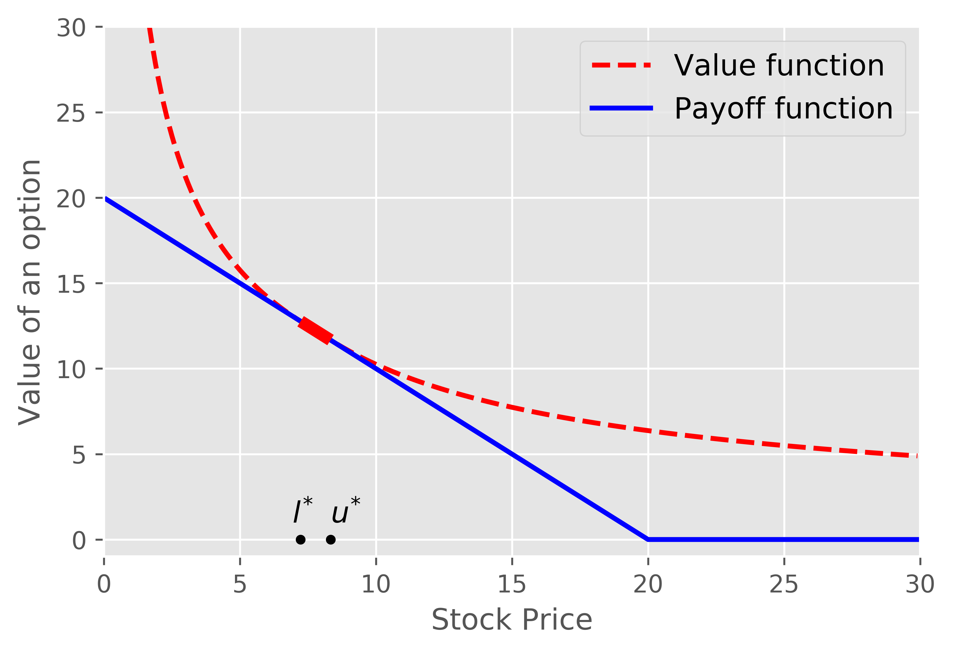
Remark 18.
Let us note that which means that the price of the option is unlimited even for an arbitrarily low stock price. This is obviously a consequence of the fact that for the discount function is strictly negative.
3.2. Exponential crashes market revisited
Let
where is some positive constant. Note that this discount function is nonegative. Hence from Theorem 15 it follows that . Let
| (47) |
From Theorem 15 (see equation (33)) with and using (16) and (17) we can conclude that
where
and from (34)
From Theorem 16 it follows that solves the following ordinary differential equation
| (48) |
with , and . The above equation is also satisfied by .
The solution to (48) is of the form
where , , and , while and are the constants that can be found based on the initial conditions (49). A similar expression can be found for with constants and satisfying (50). Having the both forms of and and by shifting these scale functions by we can produce figures of and . Taking into account the asymptotic behaviour of we can calculate the constant . It has the following form
Finally, using the continuous fit condition (35) we can find the optimal .
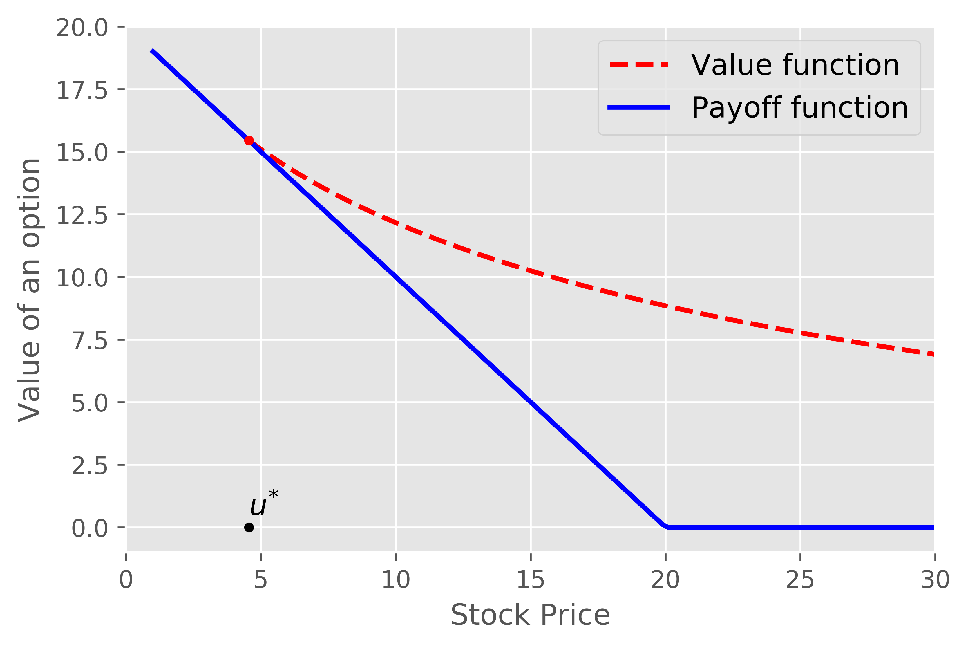
Let us assume that , , , , . The continuous fit property produces . Figure 2 shows the obtained value function.
Remark 19.
In the example above we have provided the analytical form of . However, if we choose a more complex function and we are not be able to obtain the analytical form of by solving a differential equation, we can try to solve it numerically to receive , and . In this example, we used both of these methods and we obtained the same result.
4. Proofs
Before we prove main Theorem 2 we show the convexity of European option price defined in (2) as a function of . It is done in Theorems 20 and 23. In the proof we apply idea demonstrated in [38, Prop. 4.1]. Later, in the proof of Theorem 2, we use a variant of the maximum principle.
Let us introduce a set . We use the following notations
- •
is the set of locally Hölder() functions with ,
- •
is the set of functions of at most polynomial growth in ,
- •
is the set of functions for which all the derivatives with and exist in the interior of and have continuous extensions to ,
- •
and are the sets of functions for which all the derivatives with and belong to and , respectively.
We need the following conditions in the proofs.
Assumptions (B)
There exist constants and such that
- (B1)
;
- (B2)
for all ;
- (B3)
;
- (B4)
with the Hölder continuity being uniform in ;
- (B5)
for all ;
- (B6)
;
- (B7)
is Lipschitz continuous;
- (B8)
.
Assumptions (C)
There exist a constant such that
- (C1)
, for all ;
- (C2)
, for all ;
- (C3)
, for all ;
- (C4)
, for all ;
- (C5)
.
Theorem 20.
Let all assumptions of Theorem 2 be satisfied. We assume additionally that conditions (B) and (C) hold true. Then is convex with respect to at all times .
Proof.
The first part of the proof proceeds in a similar way as the proof of [38, Prop. 4.1].
Let
where is the linear second-order differential operator of the form
with and is the integro-differential operator given by
Lemma 21.
Let Assumptions (A) and (B) hold and assume that the stock price process follows (5). Then and it is the solution to the Cauchy problem
| (51) |
Lemma 22.
Let Assumptions (A), (B) and (C) hold and assume that the stock price process follows (5). Then there exist constants and such that the value function satisfies
for all .
Proofs of both above lemmas are given in Appendix.
We introduce the function of the form
and we prove convexity of with respect to . Note that it is equivalent to the convexity of the value function in . Furthermore, based on Lemma 21, the function solves the Cauchy problem of the form
where
with . Observe that by Lemma 22 there exist constants and such that
| (52) |
for all .
Let us now define a convex function of the form
with
and
The assumptions that we put on the coefficients , and and function and their derivatives imply that each component of the above expression grows at most like for large and like for small . The same behaviour characterises .
In addition, we define the function given by
which also behaves like at and .
Hence we claim that there exist a positive constant such that
| (53) |
In the second part of the proof, we define the auxiliary function
| (54) |
for some .
We carry out a proof by contradiction. Let us then assume that is not convex. For this purpose, we denote by the set of points for which is not convex, i.e.
and we assume that the set is not empty.
From Lemma 22 we know that satisfies (52). Due to this fact and using (54) we claim that there exist a positive constant such that . This is a direct consequence of such a choice of in (54) so that grows faster than for both large and small values of .
Consequently, the set is a bounded set. Since the closure of a bounded set is also bounded, we conclude that the closure of , i.e. , is compact.
Due to the fact that a compact set always contains its infimum we can define
From the initial condition, i.e. and convexity of we have
for all . Hence we can conclude that .
Moreover, at the point when the infimum is attained, i.e. for some
This is a consequence of the continuity of the function in . In addition, for we have and thus, by applying the symmetry of second derivatives at , we derive
| (55) |
Furthermore, at we also have
Since and has a local minimum at , we have and . Thus
Since is convex in and , applying (8) we can conclude that the integral part of the above expression is nonnegative. Moreover, the concavity of and (9) imply that
| (56) |
Combining (53) with (55) and (56) at we derive that
which is a contradiction. This confirms that the set is empty, and thus is a convex function. Finally, letting we conclude that is convex in for all . ∎
Using the same arguments like in the proof of [38, Thm. 4.1], we can resign from Assumptions (B) and (C) in Theorem 20, that is, the following theorem holds true.
Theorem 23.
Let assumptions of Theorem 2 hold true. Then is convex with respect to at all times .
We are ready to give the proof of our first main result.
Proof of Theorem 2.
As noted in [38, Sec. 7], under conditions (A1)–(A4), for each there exists a constant such that the stock price process given in (5) satisfies
Together with (A5) and (A6) it implies that the value function given by
is well-defined, where is the family of -stopping times with values in for fixed maturity . Moreover, we denote
Let us define now a Bermudan option with the value function of the form
where is the set of stopping times with values in
where is some positive integer number. To simplify the notation, we denote
In contrast to the American options, the Bermudan options are the options that can be exercised at one of the finitely many number of times.
Now we show that inherits the property of convexity from its European equivalent . Next, we generalise this result to the American case .
Lemma 24.
Let assumptions of Theorem 2 hold true. Then is convex with respect to at all times .
Its proof is given in Appendix.
As the possible exercise times of the Bermudan option get denser, the value function converges to . To formalise this result, we proceed as follows. For a given stopping time that takes values in , we define
Then is a stopping time and almost surely as . Moreover, by the dominated convergence theorem, we obtain
as . Therefore, it follows that
Since it is obvious that
we finally derive
as . To receive our claim we take the maturity tending to infinity. ∎
Proof of Theorem 7.
Before we proceed to the actual proof let us remind the main exit identities from [54]. Let
for some . Then for the function defined in (47) we have
| (57) | ||||
| (58) |
where and we use condition for all and some constant in the first identity. Denoting
and keeping in mind that , from (57) and (58) we can conclude that
| (59) | ||||
where and the functions , , were defined in (16), (17) and (18).
We consider three possible cases of a position of the initial state of the process .
- (1)
: As the process is spectrally negative and starts below the interval , it can enter this interval only in a continuous way and hence and . Thus from (59)
- (2)
: If the process starts inside the interval which is an optimal stopping region, we decide to exercise our option immediately, i.e. . Therefore, we have
- (3)
: There are three possible cases of entering the interval by the process when it starts above : either enters continuously going downward or it jumps from to or jumps from the interval to the interval and then, later, enters continuously.
We can distinguish these cases in the following way
| (60) | ||||
To analyse the first component in (60), note that
We express now above formulas in terms of process. Let and we recall that in (47) we introduced functions and Then
| (61) | ||||
From the compensation formula for Lévy processes given in [50, Thm. 4.4] we have
| (62) |
where is the resolvent density of killed by potential and on exiting from positive half-line which is, by [54, Thm. 2.2], given by
Note that for given in (22).
To find , we consider
for some . Note that using the change of measure given in (20) it is equal to
| (63) |
where is the expectation with respect to and . From (58) we know that
Moreover, observe that
Furthermore, the second component of (60) is equal to
| (66) | ||||
Now we have to express all scale functions in terms of the scale functions defined in (16)–(19) with and using (47). Finally, using (60) together with (61), (62), (64) and (66) completes the proof of the first part of the theorem. If then we can proceed as before except that we do not need identity (59) and hence assumption (23) is indeed superfluous. ∎
Proof of Theorem 9.
From the facts that and that the Lévy process is right-continuous and left-continuous over stopping times, using classical arguments, we can conclude that solves uniquely equation (24); see [63, Thm. 2.4, p. 37] and [3] for details. More formally, our function as a convex function is continuous (in whole domain). Since our boundary is sufficiently regular we know that the Dirichlet/Poisson problem can be solved uniquely in . This solution can then be identified with the value function itself using the stochastic calculus or infinitesimal generator techniques in the continuation set; see [63, p. 131] for further details. Similar considerations have been performed only for a local operator in [69, Thm. 1]. Note that we can handle the non-local case of only thanks to proving the convexity of the value function first. We are left with the proof of the smoothness at the boundary of stopping set. We prove it at . The proof at lower end follows exactly in the same way. We choose to follow the idea given in [52] although one can also apply [3] or similar arguments as the ones given in [29].
Suppose then that is regular for . Since and , we have
Hence
To get the opposite inequality we introduce
By assumed regularity, a.s. as . Moreover, by Markov property
Then by (B5) and the space homogeneity of ,
and
where we use the fact that is continuously differentiable at in the last step. This completes the proof. ∎
Proof of Theorem 11.
We recall that
where . By our assumption for general Lévy process we can define a new measure via
see also (20) (considered there only for spectrally negative Lévy process). Then
| (67) | |||||
where and is the dual process to and from [29, 42, 61] it follows that under it is again Lévy process with the triple for defined in (26). This completes the proof of identity (25). Now, we recall that from general stopping theory we know that optimal stopping region for the call option is of the form for some stopping set ; see e.g. [63, Thm. 2.4, p. 37]. Performing the same transformation like it is done in (67) with instead of we can conclude that the optimal stopping time for the call option is the same as the stopping time for the put option (replacing in this transformation on the right-hand side), where . But from Theorem 5 it follows that the optimal stopping time for the put option is the first entrance time to some optimal interval. Thus from above considerations it follows that the stopping region for the call option is of the same type as for the put option and therefore (27) follows from (25). ∎
Proof of Theorem 13.
We prove that for the function satisfying (29) we have
| (68) |
Since process is continuous in Black-Scholes model, equals either to or depending on the initial state of . We can distinguish three possible scenarios
- (1)
: As the process is a continuous process and starts below the interval , then and . Thus, we get
(69) - (2)
: If the process starts inside the interval which is the optimal stopping region, we decide to exercise our option immediately, i.e. . Therefore, we have
(70) - (3)
: Similarly to the case when , the process can enter only via and thus and . Therefore,
(71)
Identities (69), (70) and (71) give the first part of the assertion of the theorem. Note that boundary condition (30) follows straightforward from the definition of the value function of the American put option.
We are left with the proof of (68). Consider strictly positive and bounded by some function . Then by [61, Prop. 3.2] the process
is a mean-one local martingale, where in the case of Black-Scholes model
Observe that equation (29) is equivalent to
Let
for some fixed . Applying the optional stopping theorem for bounded stopping time, we derive
| (72) |
We rewrite the left side of (72) as a sum of the following two components
We prove now that and . Let us define the last time when value function (4) is positive by
It easy to notice that . Then, from the boundedness of , lower boundedness of and Cauchy–Schwarz inequality we obtain
where . Note that by [10, Thm. 2] because for any . Thus . Moreover,
Hence by (72) and the dominated convergence we get (68) as long as is positive and bounded. Finally, since equals either to or , the boundedness assumption could be skipped. This completes the proof. ∎
Proof of Theorem 15.
From Theorem 2 and Remark 3 it follows that the optimal exercise time is the first entrance to the interval and by Theorem 5 the value function is equal to the maximum over and of defined in (4). We recall the observation that if the discount function is nonnegative, then it is never optimal to wait to exercise option for small asset prices, that is, always in this case and the stopping region is one-sided. We find now function in the case of (i) and (ii).
If , by the lack of memory of exponential random variable, using similar analysis like in the proof of Theorem 7, we have
Observing that
completes the proof of part (i).
If then
The first increment can be analysed like in the case of . The expression for the second component follows from (65).
Finally, the smooth fit condition follows straightforward from Theorem 9. ∎
Proof of Theorem 16.
Assume first that . Then
| (73) |
with . To produce ordinary differential equation for we start from equation (12). Putting (73) there gives
| (74) |
Taking the derivative of both sides gives
| (75) |
From (74) we have
We put it into (75) and derive
We take the derivative of both sides again to get equation (39).
Similar analysis can be done for the scale function producing equation (39) and its initial conditions. This completes the proof of the case (i).
In the case when observe that
| (76) |
with . Thus, from (12) satisfies the following equation
We simplify it deriving
| (77) |
In the next step we take derivative of both sides to get
| (78) |
From (77) we have
We put it into (78) deriving
| (79) |
5. Appendix
Proof of Lemma 21.
Firstly, we define the function of the form
such that and for all .
Taking and applying Itô’s lemma on (5), we obtain
where
We define also the function
and
We can now verify that the functions , , and satisfy conditions from [65, Section 2]. Let
From [65, Theorem 3.1] it follows that is a viscosity solution to
| (81) |
where
with
and
In addition, using [65, Prop. 3.3] yields that and it satisfies
| (82) |
for some and for all and . Based on (82) and assumptions put on we can conclude that . Then applying [44, Thm. A.14] give us the existence of a unique classical solution to (81) such that . In view of the fact that is continuous, we can observe that is Lipschitz continuous in , uniformly in . Hence from [65, Lem. 3.1] we know that that is also Lipschitz continuous in , uniformly in . From the uniqueness result given in [65, Thm. 4.1] we can deduce that . Applying [44, Thm. A.18.] we find that . Changing back to the original coordinates, it follows that and it satisfies (51). ∎
Proof of Lemma 22.
The proof follows in the same way as the proof of Lemma 21. However, this time we apply [44, Thm. A.20] which guarantees the existence of a unique classical solution to (81) satisfying . Hence, coming back to the original coordinates, we have that . Therefore, there exist constants and such that
for all . This completes the proof. ∎
Proof of Lemma 24.
By the dynamic programming principle formulated e.g. in [37], the value function satsifies
- (1)
At time , the value function is equal to .
- (2)
Given the price at the time , the price at time is .
Thus, the price of a Bermudan option at can be calculated inductively as the maximum of the payoff function and the price of a European option with expiry and payoff function . From Theorem 20 we know that the value function of European option is convex in provided the payoff function is convex, and since the maximum of two convex functions is again a convex function, we conclude that the Bermudan option price is convex in for all .
∎
6. Concluding remarks
In this paper, we have identified the value function in the optimal stopping problem with asset-dependent discounting. We have also shown that under certain conditions we are able to obtain a closed form of the value function. We have provided some specific examples as well.
It is tempting to analyse other discount functions. For example might ba a random function or just simply a random variable dependent on the asset process . One can take other processes as a discount rate where the dependence is introduced not only via correlation between gaussian components but via common jump structure. This jump-dependence is crucial since crashes in the market affect large portion of business at the same time; see e.g. [23].
One can take a Poisson version of American options where exercise is possible only at independent Poisson epochs as well. First attempt for classical perpetual American options has been already made in [62]. We believe that present analysis can be generalised to this set-up.
Obviously, it would be good to work out details for different payoff functions, hence for various options. One could think of barrier options, Russian, Israeli or Swing options. What is maybe even more interesting for the future analysis is taking into account Markov switching markets and using omega scale matrices introduced in [27]. We expect that in this setting the optimal exercise time is also the first entrance time to the interval which ends depend on the governing Markov chain.
References
- [1] Aase, K.K. (2010). The perpetual american put option for jump-diffusions. In Endre Bjørndal, M. Bjørndal, P. M. Pardalos, and M. Rönnqvist, editors, Energy, Natural Resources and Environmental Economics, 493–507. Springer Berlin Heidelberg.
- [2] Alili, L. and Kyprianou, A. (2005). Some remarks on first passage of Lévy processes, the American put and pasting principles. The Annals of Applied Probability, 15(3), 2062–2080.
- [3] De Angelis, T. and Peskir, G. (2020). Global Regularity of the Value Function in Optimal Stopping Problems. Annals of Applied Probability, 30(3), 1007–1031.
- [4] Asmussen, S., Avram, F. and Pistorius, M. (2004). Russian and American put options under exponential phase-type Lévy models. Stochastic Processes and their Applications, 109, 79–111.
- [5] Avram, F., Kyprianou, A. and Pistorius, M. (2004). Exit problems for spectrally negative Lévy processes and applications to (Canadized) Russian options. The Annals of Applied Probability, 14(1), 215–238.
- [6] Battauz, A., De Donno, M. and Sbuelz, A. (2012). Real options with a double continuation region. Quantitative Finance, 12(3), 465–475.
- [7] Battauz, A., De Donno, M. and Sbuelz, A. (2014). Real options and American derivatives: the double continuation region. Management Science, 61(5), 1094–1107.
- [8] Battauz, A., De Donno, M. and Sbuelz, A. (2017). On the exercise of American quanto options. Preprint.
- [9] Baurdoux, E. and Kyprianou, A. (2008). The McKean stochastic game driven by a spectrally negative Lévy process. Electronic Journal of Probability, 8, 173–197.
- [10] Baurdoux, E. (2009). Last exit before an exponential time for spectrally negative Lévy processes. Journal of Applied Probability, 46(2), 542–558.
- [11] Beibel, M. and Lerche, R. (2001). Optimal Stopping of Regular Diffusions under Random Discounting. Theory of Probability & Its Applications, 45(4), 547–557.
- [12] Bensoussan, A. and Lions, J.L. (1987). Impulse Control and Quasi Variational Inequalities. Wiley, New York
- [13] Bergenthum, J. and Ruschendorf, L. (2006). Comparison of option prices in semimartingale models. Finance and Stochastics, 10, 222–249.
- [14] Bergman, Y.Z., Grundy, B.D. and Wiener, Z. (1996). General properties of option prices. Journal of Finance, 51, 1573–1610.
- [15] Boyarchenko, S.I. and Levendorskii, S.Z. (2002). Perpetual American options under Lévy processes. SIAM Journal of Control and Optimization, 40, 1663–1696.
- [16] Broadie, M. and Detemple, J. (1995). American Capped Call Options on Dividend–Paying Assets. Review of Financial Studies, 8(1), 161–191.
- [17] Carr, P. and Chesney, M. (1996). American put call symmetry. Preprint.
- [18] Carr, P., Madan, D., Geman, H. and Yor, M. (2002). The fine structure of asset returns, an empirical investigation. Journal of Business, 75(2), 305–332.
- [19] Carr, P. and Linetsky, V. (2000). The valuation of executive stock options in an intensity-based framework. Review of Finance, 4(3), 211–230.
- [20] Chan, T. (2005). Pricing Perpetual American options driven by spectrally one–sided Lévy processes. Exotic Option Pricing and Advanced Lévy Models, ed. Kyprianou. John–Wiley and Sons Inc., England, 195-–216.
- [21] Chen, X., Chadam, J., Jiang, L. and Zheng, W. (2008). Convexity Of The Exercise Boundary Of The American Put Option On A Zero Dividend Asset. Mathematical Finance, 18(1), 185–197.
- [22] Chesney, M. and Jeanblanc, M. (2004). Pricing American currency options in an exponential Lévy model. Applied Mathematical Finance, 11, 207–225.
- [23] Christensen, K., Oomen, R.C.A. and Renó, R. (2018). The drift burst hypothesis. Available at SSRN.
- [24] Churiwal, A. and Shreni, A. (2012). Surveying the Indian gold loan market. Cognizant 20-20 Insights.
- [25] Cohen, S., Kuznetsov, A., Kyprianou, A. and Rivero, V. (2013). Lévy Matters II. Berlin, Heidelberg: Springer.
- [26] Cont, R. and Tankov, P. (2004). Financial Modelling with Jump Processes. Boca Raton, FL: Chapman & Hall.
- [27] Czarna, I., Kaszubowski, A., Li, S. and Palmowski, Z. (2020). Fluctuation identities for omega-killed Markov additive processes and dividend problem. Advances in Applied Probability, 52(2).
- [28] Davydov, D., Linetsky, V. and Lotz, C. (1999). The Hazard-rate Approach to Pricing Risky Debt: Two Analytically Tractable Examples. Report, Northwestern University.
- [29] De Donno, M., Palmowski, Z. and Tumilewicz, J. (2020). Double continuation regions for American and Swing options with negative discount rate in Lévy models. Mathematical Finance, 30(1), 196–227.
- [30] Detemple, J. and Kitapbayev, Y. (2018). American Options with Discontinuous Two–Level Caps. SIAM Journal on Financial Mathematics, 9(1), 219–250.
- [31] Detemple, J. (2001). American options: symmetry properties. In Musiela Jouini, Cvitanić, editor. Option pricing, interest rates and risk management, 67–104. Cambridge University Press.
- [32] Detemple, J. (2014). Optimal exercise for derivative securities. Annual Review of Financial Economics, 6, 459–487.
- [33] Detemple, J., Abdou, S.L. and Moraux, F. (2020). American step options. European Journal of Operational Research, to appear.
- [34] Eberlein, E. and Keller, U. (1995). Hyperbolic distributions in finance. Bernoulli, 1, 281–299.
- [35] Eberlein, E. and Papapantoleon, A. (2005). Symmetries and pricing of exotic options in Lévy models. In Wilmott Kyprianou, Schoutens, editor, Exotic Option Pricing and Advanced Lévy Models. Wiley Finance.
- [36] Ekström, E. Janson, S. and Tysk, J. (2005). Superreplication of options on several underlying assets. Journal of Applied Probability, 42, 27–38.
- [37] Ekström, E. (2004). Properties of American option prices. Stochastic Processes and their Applications, 114(2), 265–278.
- [38] Ekström, E. and Tysk, J. (2007). Properties of option prices in models with jumps. Mathematical Finance, 17(3), 381–397.
- [39] Ekström, E. and Tysk, J. (2007). Convexity preserving jump–diffusion models for option pricing. Journal of Mathematical Analysis and Applications, 330(1), 715–728.
- [40] El Karoui, N., Jeanblanc-Picque, M. and Shreve, S. (1998). Robustness of the Black and Scholes formula. Mathematical Finance, 8, 93–126.
- [41] Hobson, D. (1998). Volatility misspecification, option pricing and superreplication via coupling. Annals opf Applied Probability, 8, 193–205.
- [42] Fajardo, J. and Mordecki, E. (2006). Symmetry and duality in Lévy markets. Quantitative Finance, 6(3), 219–227.
- [43] Itô, K. and McKean, H. P. (1965). Diffusion Processes and Their Sample Paths. Springer-Verlag, Berlin.
- [44] Janson, S. and Tysk, J. (2004). Preservation of convexity of solutions to parabolic equations. Journal of Differential Equations, 206(1), 182–226.
- [45] Janson, S. and Tysk, J. (2003). Volatility time and properties of options. Annals of Applied Probability, 13, 890–913.
- [46] Kijima, M. (2002). Monotonicity and convexity of option prices revisited. Mathematical Finance, 12, 411–425.
- [47] Klimsiak, T. and Rozkosz, A. (2018). The valuation of American options in a multidimensional exponential Lévy model. Financial Mathematics, 28(4), 1107–1142.
- [48] Koponen, I. (1995). Analytic approach to the problem of convergence of truncated Lévy flights towards the Gaussian stochastic process. Physical Review E, 52, 1197–1199.
- [49] Krylov, N. (1980). Controlled Diffusion Processes. Springer Verlag.
- [50] Kyprianou, A. (2006). Introductory Lectures on Fluctuations of Lévy Processes with Applications. Berlin, Heidelberg: Springer–Verlag Berlin Heidelberg.
- [51] Kyprianou, A. and Surya, B. (2007). Principles of smooth and continuous fit in the determination of endogenous bankruptcy levels. Finance and Stochastics, 11(1), 131–152.
- [52] Lamberton, D. and Mikou, M. (2012). The smooth-fit property in an exponential Lévy model. Journal of Applied Probability, 49(1), 137–149.
- [53] Lamberton, D. (2009). Optimal stopping with irregular reward functions. Stochastic Processes and their Applications, 119, 3253–3284.
- [54] Li, B. and Palmowski, Z. (2018). Fluctuations of omega–killed spectrally negative Lévy processes. Stochastic Processes and Their Applications, 128(10), 3273–-3299.
- [55] Linetsky, V. (1999). Step options. Mathematical Finance 9, 55–96.
- [56] Long, M. and Zhang, H. (2019). On the optimality of threshold type strategies in single and recursive optimal stopping under Lévy models. Stochastic Processes and their Applications, 129(8), 2821–2849.
- [57] Madan, D.B. and Seneta, E. (1990). The variance gamma model for share market returns. Journal of Business, 63, 511–524.
- [58] Merton, R. (1976). Option pricing when underlying stock returns are discontinuous. Journal of Financial Economics, 3(1-2), 125–144.
- [59] Mordecki, E. (2002). Optimal stopping and perpetual options for Lévy processes. Finance and Stochastics, 6(4), 473–493.
- [60] Nielssen, O.B. (1998). The McKean stochastic game driven by a spectrally negative Lévy process. Finance and Stochastics, 1, 41–68.
- [61] Palmowski, Z. and Rolski, T. (2002). A technique for exponential change of measure for Markov processes. Bernoulli, 8(6), 767–785.
- [62] Palmowski, Z., Pérez, J.L. and Yamazaki, K. (2020). Double continuation regions for American options under Poisson exercise opportunities. Submitted for publication.
- [63] Peskir, G. and Shiryaev, A. (2006). Optimal Stopping and Free–Boundary Problems. Basel: Birkhäuser Verlag.
- [64] Pham, H. (1997). Optimal stopping, free boundary, and American option in a jump-diffusion model. Applied mathematics and optimization, 35(2), 145–164.
- [65] Pham, H. (1998). Optimal Stopping of Controlled Jump Diffusion Processes: A Viscosity Solution Approach. Journal of Mathematical Systems, Estimation, and Control 8, 1–27.
- [66] Rodosthenous, N. and Zhang, H. (2018). Beating the omega clock: An optimal stopping problem with random time-horizon under spectrally negative Lévy models. Annals of Applied Probability, 28(4), 2105–2140.
- [67] Sato, K. (1999). Lévy Processes and Infinitely Divisible Distributions. Cambridge Univeristy Press.
- [68] Schoutens, W. (2003). Lévy Processes in Finance: Pricing Financial Derivatives. Wiley.
- [69] Strulovici, B. and Szydlowski, M. (2015). On the smoothness of value functions and the existence of optimal strategies in diffusion models. Journal of Economic Theory 159, 1016–1055.
- [70] Trigeorgis, L. and Tsekrekos, A.E. (2018). Real options in operations research: A review. European Journal of Operational Research, 270(1), 1–24.
- [71] Xia, J. and Zhou, X. (2007). Stock Loans. Mathematical Finance, 17(2), 307–317.