Statistical inference for unknown parameters of stochastic SIS epidemics on complete graphs

In this paper, we are concerned with statistical inference for unknown parameters of stochastic susceptible-infectious-susceptible (SIS) epidemics on complete graphs with large degrees. For integer $n\geq 2$, a complete graph $C_{n}$ is a graph with $n$ vertices, where any two vertices are connected with an edge. A stochastic SIS epidemic model on $C_{n}$, which is also named as a contact process (see Section 6 of Liggett’s book [9]), is a continuous time Markov process with state space $\wp(C_{n}):=\{A:~A\subseteq C_{n}\}$. Let $A_{t}$ be the state of the process at moment $t$ for $t\geq 0$, then $\{A_{t}\}_{t\geq 0}$ evolves as follows. For any $x\in C_{n}$ and $t\geq 0$,

where $|A|$ is the cardinality of a set $A$ while $\lambda,\theta$ are two parameters called ‘infection rate’ and ‘recovery rate’ respectively. Note that an event occurs at rate $r$ for some $r>0$ means that the random time we wait for the event to occur follows exponential distribution with parameter $r$.

Intuitively, $\{A_{t}\}_{t\geq 0}$ describes the spread of a susceptible-infectious-susceptible epidemic on $C_{n}$. Vertices in $A_{t}$ are infectious at moment $t$ while those out of $A_{t}$ are susceptible. An infectious vertex becomes susceptible at rate $\theta$ while a susceptible vertex is infected at rate proportional to the number of infectious neighbours, which is $|A_{t}|$ since any two vertices on the complete graph are neighbours.

In this paper, we consider $\theta$ and $\lambda$ as unknown parameters which do not rely on $n$. The aim of this paper is to give consistent estimations $\widehat{\lambda}$ and $\widehat{\theta}$ of $\lambda$ and $\theta$ respectively by observing the path of $\{A_{t}\}_{0\leq t\leq T_{0}}$ for large $n$ and given moment $T_{0}>0$. Furthermore, we will establish central limit theorem and moderate deviation principle for $\widehat{\lambda}$ and $\widehat{\theta}$. For mathematical results and their applications, see next section.

Note that $C_{n}$ is a finite graph while $\emptyset$ is an absorbed state of the process. If we fix $n$ while let $t$ grow to infinity, we can only find that all the vertices are susceptible eventually. That’s why in our setting we fix the moment $T_{0}$ while let the scale of the graph grow to infinity. The other setting where the graph is fixed while time $t$ grows to infinity can be investigated when the graph is infinite. For related literatures, see References [1, 4, 5, 6, 8, 10, 11, 14] and so on.

In this section we give our main results and some of their applications. From now on we let $T_{0}>0$ be a fixed given moment and assume that

i.e., all the vertices are infectious initially. First we give consistent estimations of $\lambda$ and $\theta$. For this purpose, we define

for $x,y>0$. It is easy to check that $K(x,y)$ is continuous and strictly increasing with $y$, so it is reasonable to define $H(x,z)=H(x,\cdot)(z)$ as the inverse function of $K(x,\cdot)(y)$, i.e.,

When we need to distinguish different $C_{n}$s, we write $A_{t}$ as $A_{t}^{n}$. For each $n\geq 1$, we define

where $|A|$ is the cardinality of the set $A$. That is to say, $X_{n}$ is the number of infectious vertices at moment $T_{0}$ while $V_{n}$ is the number of vertices maintaining infectious during $[0,T_{0}]$. Note that $X_{n}$ and $V_{n}$ are statistics which can be observed directly according to the trajectory of $\{A_{t}^{n}\}_{0\leq t\leq T_{0}}$.

We define

then we have the following result, which gives consistent estimations of $\theta$ and $\lambda$.

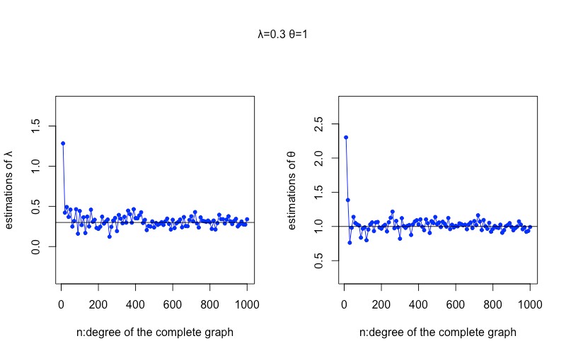
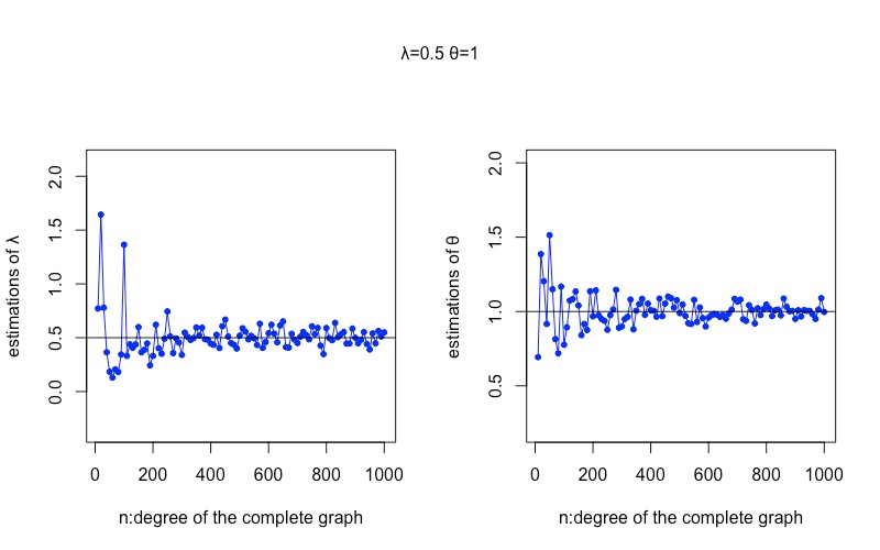
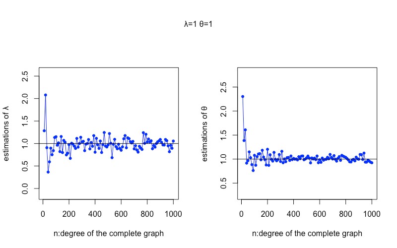
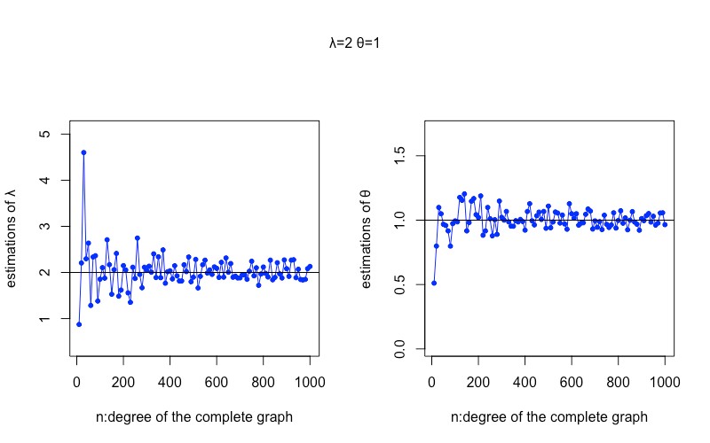
By Theorem 2.1, for the contact process on $C_{n}$ where $n$ is large and all the vertices are infectious initially, we can give estimations of $\lambda$ and $\theta$ with small errors by observing the trajectory of $\{A_{t}^{n}\}_{0\leq t\leq T_{0}}$ and then recording $X_{n}$ and $V_{n}$. Note that the advantage of this approach is that we do not need to observe this contact process for a long time. Following are simulation results of $\hat{\lambda}_{n},\hat{\theta}_{n},$ under four different settings of $\lambda,\theta$ for $20\leq n\leq 1000$ and $T_{0}=1$.

Setting 1 $\lambda=0.3$ and $\theta=1$.

Setting 2 $\lambda=0.5$ and $\theta=1$.

Setting 3 $\lambda=1$ and $\theta=1$.

Setting 4 $\lambda=2$ and $\theta=1$.

Our next theorem gives the central limit theorem of $\hat{\lambda}_{n}$ and $\hat{\theta}_{n}$. To give our result, we need to introduce some notations and definitions. Let $M_{1},M_{2}$ be $2\times 2$ matrices defined as

We then use $M_{3}$ to denote $M_{1}M_{2}$, i.e.,

We use $\mathsf{T}$ to denote the transposition operator. For later use, we define

while

For $0\leq t\leq T_{0}$ and our two unknown parameters $\lambda,\theta$, we define $v_{t}(\theta)=e^{-\theta t}$ and

For $0\leq t\leq T_{0}$, we define $M_{4}(t)$ as the $2\times 2$ symmetric matrix such that

and $M_{5}(t)$ as the $2\times 2$ matrix such that

where $\nabla=(\frac{\partial}{\partial x},\frac{\partial}{\partial y})^{\mathsf{T}}$. Then we let $\{Y_{t}\}_{t\geq 0}$ be the time-inhomogeneous $2-$dimensional O-U process such that

where $\{B_{t}\}_{t\geq 0}$ is a standard $2-$dimensional Brownian motion. As a result, $Y_{t}$ follows a Gaussian distribution $\mathbb{N}(\mathbf{0},\Sigma_{t})$ for all $0<t\leq T_{0}$, where $\Sigma_{t}$ is a $2\times 2$ positive definite matrix for every $t$. Now we can give our central limit theorem.

Theorem 2.2 can be utilized in hypothesis testings of $\lambda$ and $\theta$. For example, let $\lambda_{0}$ be a known given constant and we discuss the hypothesis testing

Since $\left(M_{3}\Sigma_{T_{0}}M^{\mathsf{T}}_{3}\right)(1,1)$ relies on $(\lambda,\theta)$, we write it as $\left(M_{3}\Sigma_{T_{0}}M^{\mathsf{T}}_{3}\right)(1,1,\lambda,\theta)$. Then, by Theorems 2.1 and 2.2, under $H_{0}$,

approximately follows standard Normal distribution $\mathbb{N}(0,1)$ for large $n$. Consequently, let

then $W$ is an approximated reject region at significant level $0.05$.

Our last result is about moderate deviation principles of $\hat{\lambda}_{n}$ and $\hat{\theta}_{n}$. Let $\{a_{n}\}_{n\geq 1}$ be a given positive sequence such that $\lim_{n\rightarrow+\infty}\frac{a_{n}}{n}=0$ while $\lim_{n\rightarrow+\infty}\frac{a_{n}}{\sqrt{n}}=+\infty$ (e.g. $a_{n}=n^{2/3}$), then we have the following result.

We can utilize Theorem 2.3 to give confidence intervals of $\lambda$ and $\theta$. For example, let $a_{n}=n^{\alpha}$ with $\alpha\in(\frac{1}{2},1)$ and $\epsilon=1$, then, by Theorem 2.3,

is a confidence interval of $\lambda$ at confidence level about $1-e^{-I_{1}(1)n^{2\alpha-1}}$. Note that the above confidence interval has the advantage that the length of the interval grows to $0$ meanwhile the confidence level grows to $1$ exponentially as $n\rightarrow+\infty$. Following are simulation results of the above confidence intervals for $\lambda=2,\theta=1,T_{0}=1$, $20\leq n\leq 1000$ and $\alpha=\frac{3}{4},\frac{2}{3},\frac{3}{5},\frac{11}{20}$ respectively.

In this section, we give outlines of the proofs of our main theorems. We mainly utilize the theory of density-dependent Markov chains introduced in [7] and Chapter 11 of [3] authored by Ethier and Kurtz. As a preparation, we recall the definition of density-dependent Markov processes. For each integer $n\geq 1$, the density-dependent Markov process $\{\xi_{t}^{n}\}_{t\geq 0}$ is a continuous-time Markov process with state space $\mathbb{R}^{d}$ for some $d$. The transition rates functions of $\{\xi_{t}^{n}\}_{t\geq 0}$ is given by

for any $l\in\mathcal{D}$, where $\mathcal{D}$ is a given subset of $\mathbb{R}^{d}$ while $\{F_{l}\}_{l\in\mathcal{D}}$ are smooth functions from $\mathbb{R}^{d}$ to $[0,+\infty)$. To illustrate the relation between density-dependent Markov chains and our SIS epidemic model, we define

Specially, $X_{T_{0}}^{n}=X_{n}$ and $V_{T_{0}}^{n}=V_{n}$, where $X_{n},V_{n}$ are defined as in Section 2. Let $\zeta_{t}^{n}=\left(X_{t}^{n},V_{t}^{n}\right)^{\mathsf{T}}$, then, according to the transition rates functions of $\{A_{t}^{n}\}_{t\geq 0}$, it is easy to check that $\{\zeta_{t}^{n}\}_{t\geq 0}$ is a version of density-dependent Markov chain with $d=2$,

and $F_{l_{i}}=F_{i}$ for $i=1,2,3$, where $l_{1},l_{2},l_{3}$ and $F_{1},F_{2},F_{3}$ are defined as in Section 2.

We recall the law of large numbers and cental limit theorem of density-dependent Markov chains introduced in [7] by Kurtz. Note that vectors appear in following propositions are all column vectors.

Now we can give proofs of our first and second main results.

References

- [1] Becker, N. (1977). Estimation for discrete time branching processes with application to epidemics. Biometrics 33, 515-522.
- [2] Dembo, A. and Zeitouni, O. (1997). Large Deviations: Techniques and Applications. Springer, Berlin.
- [3] Ethier, N. and Kurtz, T. (1986). Markov Processes: Characterization and Convergence. John Wiley and Sons, Hoboken, NJ, USA.
- [4] Fierro, R., Leiva, V. and Balakrishnan, N. (2015). Statistical inference on a stochastic epidemic model. Communications in Statistics. Simulation and Computation 44, 2297-2314.
- [5] Guy, R., Larédo, C. and Vergu, E. (2015). Approximation of epidemic models by diffusion processes and their statistical inference. Journal of Mathematical Biology 70, 621-646.
- [6] Hadeler, K. P. (2011). Parameter estimation in epidemic models: simplified formulas. Canadian Applied Mathematics Quarterly 19, 343-356.
- [7] Kurtz, T. (1978). Strong approximation theorems for density dependent Markov chains. Stochastic Processes and their Applications 6, 223-240.
- [8] Lekone, P., Finkenstädt, B. (2006). Statistical inference in a stochastic epidemic SEIR model with control intervention: Ebola as a case study. Biometrics 62, 1170-1177.
- [9] Liggett, T. M. (1985). Interacting Particle Systems. Springer, New York.
- [10] Lindenstrand, D. and Svensson, Å. (2013). Estimation of the Malthusian parameter in an stochastic epidemic model using martingale methods. Mathematical Biosciences 246, 272-279.
- [11] Pan, J., Gray, A., Greenhalgh, D. and Mao, X. (2014). Parameter estimation for the stochastic SIS epidemic model. Statistical Inference for Stochastic Processes 17, 75-98.
- [12] Pardoux, E. and Samegni-Kepgnou, B. (2017). Large deviation principle for epidemic models. Journal of Applied Probability 54, 905-920.
- [13] Xue, XF. (2018). Moderate deviations of density-dependent Markov chains. Arxiv: 1908.03762.
- [14] Yip, P. and Chen, Q. (1998). Statistical inference for a multitype epidemic model. Journal of Statistical Planning and Inference 71, 229-244.