A First-Principles Nonequilibrium Deterministic Equation of Motion of a Brownian Particle and Microscopic Viscous Drag Preprint: UATP/1904

The central concept of the NEQT exploited here is that of the internal equilibrium (IEQ) according to which the entropy $S$ of a NEQ macrostate is a state function of the state variables in the enlarged state space $\mathfrak{S}$ Gujrati-I; Gujrati-II; Gujrati-III; see Sec. II.3 for details. The enlargement of the space relative to the EQ state space $\mathfrak{S}_{0}$ is due to independent internal variables Coleman; deGroot; Prigogine; Maugin; Gujrati-I; Gujrati-II that are required to describe a NEQ macrostate as we explain below. In EQ, the internal variables are no longer independent of the observables forming the space $\mathfrak{S}_{0}$. As a consequence, their affinities vanish in EQ. Observables are quantities that can be controlled from the outside but not the internal variables. In general, the temperature $T$ of the system in IEQ is identified in the standard manner by the relation

using the fact that $S$ is state variable in $\mathfrak{S}$.

An important property of IEQ macrostates is the following that will prove very useful here: It is possible in an IEQ macrostate to have different degrees of freedom or different parts of a system to have different temperatures than $T$. For example, in a glass, it is well known that the vibrational degrees of freedom have a different temperature than the configurational degrees of freedom Debenedetti; Gujrati-Hierarchy. In the viscous drag problem, the CM-motion of the BP can be separated out from the motion of its various constituent particles as is well known; see Sec. IV. Then, it is possible for the BP motion to have a different temperature than $T$ introduced above. This observation is easily verified in MNEQT based on the concept of IEQ as done elsewhere (Gujrati-Hierarchy, see Sec. 8.1 and Eq. (58)). The derivation also works when various parts of the system have different temperatures. As this observation will play an important role in this investigation, we rederive it for clarity in a different manner, which supplements the previous demonstration Gujrati-Hierarchy and also shows how an internal variable is required to describe an IEQ macrostate.

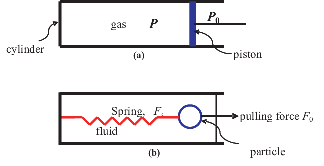
We consider a system $\Sigma$, see Fig. 1, that contains a single BP that is shown explicitly in Fig. 2 as part of $\Sigma$. The single BP is our focus in this work. We follow the standard formulation for a statistical system $\Sigma$ Landau, which interacts weakly with a much larger medium $\widetilde{\Sigma}$ so this interaction $U_{\text{int}}$ is normally ignored. This is possible as we do not allow any relative motion between $\Sigma$ and $\widetilde{\Sigma}$ as noted above; see also Sec. II.3. However, $U_{\text{int}}$ must not be zero identically otherwise there cannot be any energy (heat and work) exchange between $\Sigma$ and $\widetilde{\Sigma}$. Together, they form an isolated system $\Sigma_{0}\doteq\Sigma\cup\widetilde{\Sigma}$. The system may be far away from equilibrium so the new theory is more general than the EQ treatments by Einstein and Langevin.

As said above, treating NEQ states normally requires some (extensive) internal variables that are generated due to internal processes Coleman; deGroot; Prigogine; Maugin; Gujrati-I; Gujrati-II. Their conjugate fields, called affinity, vanish only in equilibrium. The system is specified by a Hamiltonian $\mathcal{H}(\left.\mathbf{z}\right|\mathbf{Z})$ in which $\mathbf{z}$ denotes a phase point in its phase space and $\mathbf{Z}\doteq\left\{Z\right\}$ denotes the set of parameters such as the volume $V$, the number of particles $N$ which we do not show, etc. and internal variables.

The time dependence in some or all components in $\mathbf{Z}$ gives rise to time dependence in the Hamiltonian $\mathcal{H}(\left.\mathbf{z}\right|\mathbf{Z})$; the dynamical variable $\mathbf{z}$ plays no role as we show in Eqs. (6a) and (6b). From $\mathcal{H}(\left.\mathbf{z}\right|\mathbf{Z})$, we identify microstates $\mathfrak{m}_{k}(\mathbf{Z})$ and their microenergies $E_{k}(\mathbf{Z})$; we will usually suppress the $\mathbf{Z}$-dependence unless necessary for clarity. The microstate $\mathfrak{m}_{k}$ appears with probability $p_{k}$ in the statistical ensemble. The set $\left\{p_{k}\right\}$ determines the stochasticity in the ensemble. Accordingly, it determines the nature of the macrostate (EQ vs NEQ) but the sets $\left\{E_{k}\right\}$ and $\left\{\mathfrak{m}_{k}\right\}$ are independent of $\left\{p_{k}\right\}$ so they are deterministic.

In the $\mu$NEQT, the two aspects can be separated out in an unambiguous fashion so we can uniquely determine the deterministic quantities such as $\left\{F_{k,\text{BP}}\right\}$. Accordingly, we do not need to partition microforces into “slow” and “fast” components. There is no random force in our approach so we avoid the complications of the conventional Wiener process in the Langevin approach. Clearly, the deterministic microforces are oblivious to the stochastic nature of the thermodynamic system. The second law emerges automatically after averaging, but not without it. Thus, the $\mu$NEQT as an extension of the MNEQT will be based solely on the sets $\left\{E_{k}\right\}$ and $\left\{p_{k}\right\}$ so it provides a first-principles deterministic theory from which the MNEQT is trivially reconstructed.

To investigate the ensemble, it is useful to treat a microquantity that takes values $\left\{q_{k}\right\}$ over $\left\{\mathfrak{m}_{k}\right\}$ at each instant as a random variable $\mathsf{q}$ defined over $\left\{\mathfrak{m}_{k}\right\}$. Thus, $\left\{E_{k}\right\}$ and $\left\{F_{k,\text{BP}}\right\}$ refer to the outcomes of the random variables E and F${}_{\text{BP}}$, respectively. In this study, we use sans serif typeface to denote random variables to distinguish them from their outcomes. For a given $\left\{p_{k}\right\}$, q is characterized by its ensemble average $\left\langle\mathsf{q}\right\rangle$ and various moments such as the variance $\left\langle(\Delta\mathsf{q})^{2}\right\rangle$ in terms of the fluctuation $\Delta\mathsf{q\doteq q-}\left\langle\mathsf{q}\right\rangle$. As $p_{k}$’s continue to change in a NEQ state, $\left\langle\mathsf{q}\right\rangle$ and $\left\langle(\Delta\mathsf{q})^{2}\right\rangle$ also change. In the $\mu$NEQT, the macroforce $\mathbf{F}_{\text{BP}}\doteq\left\langle\text{{F}}_{\text{BP}}\right\rangle$ corresponding to $\left\{\mathbf{F}_{k,\text{BP}}\right\}$ must oppose the motion in accordance with the second law as does $\mathbf{F}_{k,\text{f}}(t)$ but not individual $\mathbf{F}_{k,\text{BP}}$’s. The non-vanishing fluctuations, see Eqs. (34) and (35), in $\mathbf{F}_{k,\text{BP}}$ even in equilibrium (where $\mathbf{F}_{\text{BP}}=0$) demonstrates that $\mathbf{F}_{k,\text{BP}}$’s do not always oppose the motion of $\mathfrak{m}_{k}$ in the $\mu$NEQT. This effectively means that if we consider F${}_{\text{BP}}$ to be of the form $(-\mathsf{\gamma v})$, $\mathsf{v,\gamma}$ having the outcomes $\left\{v_{k}\right\},\left\{\gamma_{k}\right\}$, respectively, then $\gamma_{k}$ is of either sign.

For thermodynamic considerations, instead of considering F${}_{\text{BP}}$, we will find it convenient to consider the internal microwork $d_{\text{i}}$W${}_{\text{BP}}$ done by it with outcomes $\left\{d_{\text{i}}W_{k,\text{BP}}\right\}$, see Eq. (30). Being specific to $\mathfrak{m}_{k}$, the internal microwork $d_{\text{i}}W_{k,\text{BP}}$ also has a unique value but no specific sign; only the ensemble average $d_{\text{i}}W_{\text{BP}}\doteq\left\langle d_{\text{i}}\mathsf{W}_{\text{BP}}\right\rangle\geq 0$ in accordance with the second law as we will see. That $d_{\text{i}}W_{k,\text{BP}}$ and $\gamma_{k}$ have no sign restriction and $\mathbf{F}_{k,\text{BP}}$ does not always oppose motion is the unique feature of our approach.

We consider the two systems (a) and (b) shown in Fig. 2 as our system $\Sigma$. In (a), $P,V$ represent some generic work field and variable, which we label pressure and volume for convenience. We treat the piston or the particle as a BP. As the BP forms a subsystem, we denote it by $\Sigma_{\text{BP}}$ and the remainder of $\Sigma$ by $\Sigma_{\text{R}}$. We assume that the piston in (a) may be either mesoscopic or macroscopic, while the particle in (b) will be assumed to denote a mesoscopic particle. Thus, our approach will unify the two different scales. We will establish that both experience fluctuating Brownian motion v over $\left\{\mathfrak{m}_{k}\right\}$, except that for the macroscopic size piston, it is not noticeable because of its macroscopic mass.

We follow Einstein and focus on the BP’s center-of-mass. Let $V$ denote the volume of $\Sigma$ and $\mathbf{P}_{\text{BP}}$ and $\mathbf{P}_{\text{R}}$ the linear momenta of $\Sigma_{\text{BP}}$ and $\Sigma_{\text{R}}$, respectively. Let $\mathbf{R}_{\text{BP}}$ and $\mathbf{R}_{\text{R}}$ denote the displacement of the CM of $\Sigma_{\text{BP}}$ and $\Sigma_{\text{R}}$, respectively. This makes $\Sigma$ nonuniform and out of EQ Note. We assume $\Sigma$ stationary in the lab-frame (compare with Gujrati-II) so that

we also take $\widetilde{\Sigma}$ and, hence, $\Sigma_{0}$ to be stationary so that $\Sigma$ has no relative motion with respect to $\widetilde{\Sigma}$ and $\Sigma_{0}$ as noted above.

We will establish here that $\mathbf{P}_{\text{BP}}$ and $\mathbf{P}_{\text{R}}$ must be treated as parameters, which is in the spirit of the original assumption of Einstein about the CM-motion. As $\mathbf{P}_{\text{BP}}$ and $\mathbf{P}_{\text{R}}$ denote the total momenta that we will associate with respective CMs of $\Sigma_{\text{BP}}$ and $\Sigma_{\text{R}}$, they can only be changed by ”external” forces to the two bodies, i.e., only the force exerted by $\Sigma_{\text{R}}$ on $\Sigma_{\text{BP}}$ can change $\mathbf{P}_{\text{BP}}$, and the force exerted by $\Sigma_{\text{BP}}$ on $\Sigma_{\text{R}}$ can change $\mathbf{P}_{\text{R}}$. These forces are equal and opposite as they are internal forces for $\Sigma$, and cancel out in $\Sigma$; recall that it is stationary. Thus, we need to determine one of these forces in the following. This cancellation also applies to each microstate of $\Sigma$. However, these ”external” forces are due to some mutual interactions between the two bodies as we discuss at length in Sec. IV. In the absence of this interaction, $\mathbf{P}_{\text{BP}}$ and $\mathbf{P}_{\text{R}}$ cannot change so it is required for the viscous drag and it cannot be neglected as we have observed above.

We can treat $\Sigma_{\text{R}}$ as our medium $\widetilde{\Sigma}$ and treat $\Sigma_{\text{BP}}$ as our system $\Sigma$ with $\mathbf{P}_{\text{R}}$ replaced by the linear momentum $\widetilde{\mathbf{P}}$ of $\widetilde{\Sigma}$ if we want the BP to interact directly with $\widetilde{\Sigma}$, a case that is a trivial modification but which is usually studied (Kapral0, for example). We will discuss this situation in Sec. IV.

We use the notation

related to the second irreversible contribution in Eq. (17). It follows that for the inequality to be valid, we must have the following form for NEQ $\mathbf{F}_{\text{BP}}$ in the MNEQT

in which $f(T,\mathbf{V},t)$ must be an even scalar function of $\mathbf{V=P}_{\text{BP}}/m$ at each instant so that $d_{\text{i}}W_{\text{BP}}=f(T,\mathbf{V},t)\mathbf{V}^{2}dt\geq 0$. As $\mathbf{F}_{\text{BP}}$ opposes motion, it represents the viscous force we are interested in. Let us compare $\mathbf{F}_{\text{BP}}$ above with its definition in Eq. (14), according to which it is a derivative of $E$ with respect to $\mathbf{R}$. The only way this derivative can give a result along the direction of $\mathbf{V}$ is for the scalar function $E$ to be a function of the combination

as a scalar. We thus conclude that

so $f(T,\mathbf{V},t)$ will also include a dependence on $\mathbf{R}$ in $f$ through $u$ so we must write it as $f(T,V,u)$. Hopefully, this will make Eq. (27) suitable for some active BPs Marconi; Romanczuk; Kapral-2017; Fodor. In general, the dependence on $\mathbf{V}$ through $u$ may be very complex as will become clear in Sec. IV.

As $\mathbf{F}_{\text{BP}}$ is the macroforce corresponding to the viscous drag, the above discussion provides a thermodynamic justification of the viscous drag. To make connection with the Langevin equation, we will assume $f(u,t)$ to be a power series in $u^{2}\$with $f(0,t)=\gamma(t)\geq 0$ so that $d_{\text{i}}W_{\text{BP}}\simeq\gamma(t)\mathbf{V\cdot}d\mathbf{R}$ is the frictional work in the small-speed approximation, which will be called the Langevin limit from now on. In this limit, $d_{\text{i}}W_{\text{BP}}\simeq\gamma(t)\mathbf{V}^{2}(t)dt\geq 0$ at any instant $t$. Langevin takes $\gamma(t)$ to be a constant $\gamma$.

The above discussion also provides a thermodynamic justification of the viscous drag in the Langevin equation in the small-speed approximation. For arbitrary speeds, we can treat $f(T,u,t)$ as the analog of an effective $\gamma_{\text{eff}}$ in Eq. (2), which is a complicated function of $T,\mathbf{V}$ and $t$, a situation commonly encountered in active BPs Marconi; Romanczuk; Kapral-2017; Fodor. We will not pursue active BPs in this work except tangentially; they will be treated later.

As we will see below, we get more insight into the viscous force $\mathbf{F}_{\text{BP}}(t)$ when we consider its microanalogs $\mathbf{F}_{k,\text{BP}}(\mathbf{V,}t)$ in the $\mu$NEQT.

That the internal microwork $d_{\text{i}}W_{k\text{,BP}}$ has no sign restriction is another point of departure from Langevin’s approach and is discussed next. We focus on the form

for $\mathfrak{m}_{k}$ and determine Newton’s equation for the BP at a relative location $\mathbf{R}_{k}(t)$; $k$ on $\mathbf{R}_{k}(t)$ is added for clarity. The deterministic equation

describes the trajectory of the BP in the $\mu$NEQT. The trajectory $\mathbf{R}_{k}(t)$ is obtained by integrating twice Eq. (31) using basic calculus, and is also deterministic and at least twice differentiable. Introducing the deviation $\Delta\mathbf{F}_{k,\text{BP}}(t)\doteq\mathbf{F}_{k,\text{BP}}(t)-\mathbf{F}_{\text{BP}}(t)$, we can express $\mathbf{F}_{k,\text{BP}}(t)$ in terms of $\mathbf{F}_{\text{BP}}(t)$ as

which may suggest that $\Delta\mathbf{F}_{k,\text{BP}}(t)$ is Langevin’s $\boldsymbol{\xi}(t)$. This is where other important differences from the Langevin approach appear. The $\mathbf{F}_{\text{BP}}(t)$ is a function of the average relative velocity $\mathbf{V}(t)\equiv\left\langle\mathsf{V}(t)\right\rangle$ so it does not represent the microforce $\mathbf{F}_{k,\text{f}}(t)\$that appears in Eqs. (1-2). Furthermore, $\mathbf{F}_{k\text{,BP}}\doteq\partial E_{k}/\partial\mathbf{R}$ is deterministic in the $\mu$NEQT as noted above. So is $\mathbf{F}_{\text{BP}}(t)$. Thus, $\Delta\mathbf{F}_{k,\text{BP}}(t)$ also takes a single value for each $\mathfrak{m}_{k}$, while $\boldsymbol{\xi}(t)$ is stochastic. The stochasticity in the $\mu$NEQT emerges as we average Eq. (31) over all microstates to yield

with $\mathbf{R}(t)\doteq\left\langle\mathbf{R}(t)\right\rangle,p_{k}>0$, and a dot represents the total time derivative; the last two terms on the right side are due to temporal changes in $\left\{p_{k}\right\}$; they vanish in EQ so that we obtain a simple equation of motion for the average trajectory $\mathbf{R}(t)$ of $\mathbf{R}_{k}(t)$ that is normally discussed in the literature for the Langevin equation.

References

- (1) L.D. Landau, E.M. Lifshitz, Statistical Physics, Vol. 1, Third Edition, Pergamon Press, Oxford (1986).
- (2) A uniform system in equilibrium cannot sustain relative motions of its parts Landau.
- (3) S.R. de Groot and P. Mazur, Nonequilibrium Thermodynamics, First Edition, Dover, New York (1984).
- (4) D. Kondepudi and I. Prigogine, Modern Thermodynamics, John Wiley and Sons, West Sussex (1998).
- (5) G.A. Maugin, The Thermomechanics of Nonlinear Irreversible Behaviors: An Introduction, World Scientific, Singapore (1999).
- (6) B.D. Coleman, J. Chem. Phys. 47, 597 (1967).
- (7) P.D. Gujrati, Phys. Rev. E 81, 051130 (2010); P.D. Gujrati, arXiv:0910.0026.
- (8) P.D. Gujrati, Phys. Rev. E 85, 041128 (2012); P.D. Gujrati, arXiv:1101.0438.
- (9) P.D. Gujrati, Phys. Rev. E 85, 041129 (2012); P.D. Gujrati, arXiv:1101.0431.
- (10) A. Einstein, Ann. Phys. 17, 549, (1905), appearing in The Collected Papers of Albert Einstein, English translation by Anna Beck, Princeton U.P., Princeton, NJ. (1989), Vol. 2, pp. 123–134.
- (11) P. Langevin, C. R. Acad. Sci. (Paris) 146, 530 (1908); appears translated in English in D.S. Lemons and A. Gythiel, Am. J. Phys. 65, 1079 (1997).
- (12) S. Chandrasekhar, Rev. Mod. Phys. 21, 383 (1949).
- (13) K. Sekimoto, Stochastic Energetics, Springer, Berlin (2010).
- (14) U. M. B. Marconi, J. Chem. Phys. 124, 164901 (2006) and references therein.
- (15) P. Romanczuk, M. Bär, W. Ebeling, B. Lindner, and L. Schimansky-Geier, Eur. Phys. J. Spec. Top. 202, 1 (2012).
- (16) P. Gaspard, and R. Kapral, J. Chem. Phys. 147, 211101 (2017).
- (17) É. Fodor and M. C. Marchetti, Physica A, 504, 106 (2018).
- (18) C. Beck, Prog. Theor. Phys. Supp., 162, 29 (2006).
- (19) B. Wang, S.M. Anthony, S.C. Bae, and S. Granick, Proc. Natl. Acad. Sci., 106, 15160 (2009).
- (20) C. Xue, X. Zheng, K. Chen, Y. Tian, and G. Hu, J. Phys. Chem. Lett. 7, 514 (2016).
- (21) M.G. McPhie, P.J. Daivis, I.K. Snook, J. Ennis, and D.J. Evans, Physica A, 299, 412 (2001).
- (22) P. Gaspard, Physica A, 552, 121823 (2019).
- (23) D. Mizuno, C. Tardin, C.F. Schmidt, and F.C. MacKintosh, Science, 315, 370 (2007).
- (24) P. Hänggi and F. Marchesoni, Rev. Mod. Phys. 81, 387 (2009).
- (25) R. Huang, I. Chavez, K.M. Taute, B. Lukic, S. Jeney, M.G. Raizen, and E. Florin, Nature Phys. 7, 576 (2011).
- (26) J. Keizer, Statistical Thermodynamics of Nonequilibrium Processes, Springer-Verlag, New York (1987).
- (27) P. Mazur and D. Bedeaux, Physica A 173, 155 (1991); see also, Biophys. Chem. 41, 41 (1991).
- (28) Y. Pomeau and J. Piasecki, C.R. Physique, 18, 570 (2017).
- (29) R. Zwanzig, Nonequilibrium Statistical Mechanics, Oxford (2001).
- (30) D.J. Evans and G.P. Morriss, Statistical Mechanics of Nonequilibrium Liquids, ANU Press, Canaberra (2007).
- (31) P.D. Gujrati, arXiv:1702.00455.
- (32) P.D. Gujrati, arXiv:1803.09725; see also P.D. Gujrati, Phys. Lett. A 384, 126460 (2020).
- (33) R.I. Cukier, R. Kapral, J.R. Lebenhaft, and J.R. Mehaffey, J. Chem. Phys. 73, 5244 (1980).
- (34) L.E. Reichl, A Modern Course in Statistical Physics, Second Edition, John Wiley and Sons, New York (1998).
- (35) A change in some extensive macroquantity is Gujrati-I; Gujrati-II; Gujrati-GeneralizedWork; Gujrati-GeneralizedWork-Expanded partitioned into , which is exchanged with the medium, and , which is internally generated within the system. The second law controls the behavior of . A similar partition for a microquantity can also be carried out but is not controlled by the second law.
- (36) P.G. Debenedetti, Metastable Liquids; Conc epts and Principles, Priceton University Press, Princeton (1996).
- (37) P.D. Gujrati, Entropy, 20, 149 (2018); see Sec. 8.1 and Eq. (58).
- (38) P.D. Gujrati, arXiv:1304.3768; see also Gujrati-Entropy2.
- (39) P.D. Gujrati, Entropy, 17, 710 (2015).
- (40) L.D. Landau and E.M. Lifshitz, Fluid Mechanics, Pergamon Press, Oxford (1982).
- (41) The derivation of in Sec. 6.2 in Ref. Gujrati-Entropy2 assumes fixed macrofields with corresponding extensive microquantities fluctuating so that ; see Eq. (21). We are also interested in the ensemble with fixed extensive macroquantities but fluctuating microfields. The derivation is easily extended to handle this situation with the result given in Eq. (20).
- (42) P.D. Gujrati in Recent Research Developments in Chemical Physics, edited by S. Pandelai (Transworld Research Network, Trivandrum, Kerala, India, 2003), Vol. 4, p. 243; arXiv:cond-mat/0308439.
- (43) Y. Mishin, Annals of Physics 363, 48 (2015).
- (44) J.N. Israelachvili, Intermolecular and surface forces, Third edition, Academic Press, U.S.A. (2011).
- (45) L.V. Woodcock, Chem. Phys. Lett. 10, 257 (1971).
- (46) G. Bussi, D. Donadio, and M. Parrinello, J. Chem. Phys. 126, 014101 (2007).
- (47) H. C. Andersen, J. Chem. Phys. 72, 2384 (1980).
- (48) S. Nosé, J. Phys.: Condens. Matter, 2 (Supplement), SA115 (1990).
- (49) D. Frenkel and B. Smit, Understanding Molecular Simulation, Academic Press, San Diego (1996).
- (50) P.D. Gujrati, arXiv:1105.5549; see also Gujrati-Entropy2.
- (51) P.D. Gujrati, arXiv:1206.0702; see also Gujrati-Entropy2.