Compressed sensing-based SARS-CoV-2 pool testing

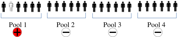
Group testing is concerned with discovering a class of interest from a larger set containing non-members of the class of interest without testing each member of the set. This is done by sub-dividing the set into subsets and testing each subset as one element. The goal is that with the number of subset/groups being far smaller than the total number of elements in the set, one is able to successfully identify the class of interest. More precisely, group testing seeks to identify $k$ members of a class of interest out of a set of $n$ elements by performing $m$ tests of $m$ groups, where $m\ll n$. In the disease identification setting, we would like to identify $k$ infected individuals from a population of $n$ individual performing $m$ group (pool) tests, again we require that $m\ll n$. The ratio $k/n$ (denoted as $p$) is known as the prevalence. Usually, group testing works well when $p$ is small. Is can be shown by a combinatorial argument that we need $\mathcal{O}\left(k\log_{2}\left(n/k\right)\right)$ tests for pool testing to work [17]. Figure 1 shows an example of pool testing to identify an infected individual. Here each individual participates in only one pool.

We can have pool testing setups where individuals participate in more than one pool. Figure 2 illustrates this with each individual participating in 2 pools. This can be represented in a 2-dimensional (2D) grid; while the example in Figure 1 can be considered 1D. Going from 1D to 2D may reduce the need to re-test.

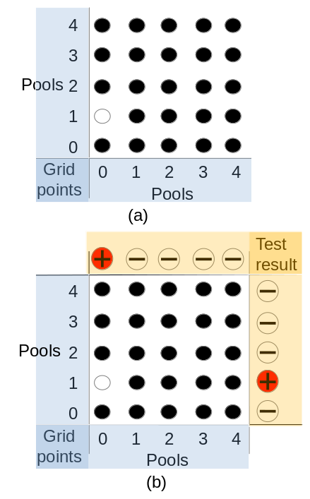
Moreover, this can be extended to a $d$-dimensional setting, where each individual will participate in $d$ pools. This is what the successfully applied hypercube method is about, see [23]²² 2 Approach being used in Rwanda.. The 1D, 2D, $\cdots,$ dD pool testing are instances of the so-called array testing, see [28].

Mathematically, we can represent the population of size $n$ by a binary vector, $\mathbf{x}\in\{0,1\}^{n}$ with $k$ ones for the infected individuals and $n-k$ zeros for the non-infected individuals. Pooling samples of a group together is equivalent to evaluating

for some appropriate binary vector ${\bf a}\in\{0,1\}^{n}$. For a matrix $\mathbf{A}\in\{0,1\}^{m\times n}$ whose rows ${\bf a}_{i}$ represent the $m$ groups, we set

The vector $\mathbf{y}$ is also referred to as the measurement/observation vector.

The recovery of the infected individuals, equivalently $\mathbf{x}$, from observing $\mathbf{y}$ and knowing $\mathbf{A}$ would lead to solving the following binary system of equations, since both $\mathbf{A}$ and $\mathbf{x}$ are binary.

The setting described above where the groups are fixed is known as the non-adaptive case of group testing. Alternatively, one may only form a group after knowing the outcome of the preceding test(s). In that case we perform adaptive group testing. Non-adaptive approaches are faster but they require more measurements than adaptive approaches. Adaptive methods achieve the optimal $\mathcal{O}\left(k\log_{2}\left(n/k\right)\right)$ number of measurements [17]; while non-adaptive methods need $\mathcal{O}\left(k^{2}\log_{k}\left(n\right)\right)$ number of measurements [1].

Many recovery algorithms for group testing have been proposed. One popular such algorithm for non-adaptive group testing is Combinatorial Orthogonal Matching Pursuit (COMP). In the noiseless setting the COMP algorithm assigns a sample as positive (i.e., infected) if and only if all the $k$ tests containing the sample satisfy $y_{m}>0$. COMP will work perfectly, if the pooling strategy is such that we have “$k$-disjunct” sets of measurements (see Definition 4.1). Another algorithm for the adaptive case, is the binary splitting algorithm by [17]. A pseudo-code for COMP is give in Algorithm 1 below.

Mathematically, compressed sensing is concerned with the construction of a linear operator and the solution of an underdetermined system of linear equations resulting from the application of the linear operator. More precisely let $\mathbf{A}\in\mathbb{R}^{m\times n}$ be our linear operator, let $\mathbf{x}\in\mathbb{R}^{n}$ be the unknown variable vector and let the application of $\mathbf{A}$ result in $\mathbf{y}\in\mathbb{R}^{m}$. Therefore, with $m\ll n$, we have an underdetermined linear system (note both $\mathbf{A}$ and $\mathbf{x}$ are real):

In compressed sensing parlance $\mathbf{A}$ is called the sensing/measurement matrix, $\mathbf{y}$ is the measurement vector and $\mathbf{x}$ is the signal of interest. Linear algebra tells us that there are infinitely many solutions to (4). However, it is possible to obtain a unique solution if we make some assumptions on $\mathbf{A}$ and $\mathbf{x}$. The main assumption on $\mathbf{x}$ is that it has some simplicity/redundancy. The simplicity of $\mathbf{x}$ is either sparsity or compressibility. By sparsity of $\mathbf{x}$ we mean it has few non-zero elements. Let $\mathcal{S}$ be the support of $\mathbf{x}$, i.e. $\mathcal{S}=\{j\penalty\ :\penalty\ x_{j}\neq 0,\penalty\ \forall j\in 1,\ldots,n\}$ and let $|\mathcal{S}|\leq k$, then $\mathbf{x}$ is $k$-sparse. Conventionally, $\|\mathbf{x}\|_{0}$ (the $\ell_{0}$-norm of $\mathbf{x}$)³³ 3 This is not a norm because $\|\lambda\mathbf{x}\|_{0}=\|\mathbf{x}\|_{0}$ for all scalars $\lambda\neq 0$ and all vectors $\mathbf{x}$. is used to represent the sparsity of $\mathbf{x}$.
Precisely,

where $\mathbb{I}$ is the indicator/characteristic function. On the other hand, $\mathbf{x}$ is said to be $k$-compressible when $\mathbf{x}$ can be approximated quite well by a $k$-sparse vector. Furthermore, $\mathbf{x}=\Psi\mathbf{z}$ is $k$-sparse ($k$-compressible) in a basis $\Psi$ when $\mathbf{z}$ is $k$-sparse ($k$-compressible). We denote the restriction of $\mathbf{x}$ on its support as $\mathbf{x}_{\mathcal{S}}\in\mathbb{R}^{k}$ and the restriction of $\mathbf{x}$ on the complement of the support as $\mathbf{x}_{\mathcal{S}^{c}}\in\mathbb{R}^{n-k}$.

The assumption on $\mathbf{A}$ is that it is an information preserving projection or a bi-Lipschitz linear metric space embedding of all $k$-sparse vectors into $\mathbb{R}^{m}$ henceforth referred to as a stable linear embedding. The conditions for $\mathbf{A}$ to fulfil the information preservation requirement include the following.

1. $(i)$

   Restricted Isometry Property (RIP). A more general definition of the RIP, i.e. $\ell_{p}$-norm restricted isometry property ($\mathrm{RIP}_{p}$) for $p>1$ is the following.

   Definition 1.2.

   Matrix $\mathbf{A}$ has $\mathrm{RIP}_{p}$ of order $k$, with constants $\delta_{k}<1$, if for all $k$-sparse $\mathbf{x}$, it satisfies

   $$(1-\delta_{k})\|\mathbf{x}\|_{p}^{p}\leq\|\mathbf{A}\mathbf{x}\|_{p}^{p}\leq(1+\delta_{k})\|\mathbf{x}\|_{p}^{p}.$$

   (6)

   For small $\delta_{k}$, we have $\mathbf{A}$ being a near isometry and this implies that it a information preserving. Note that $p=2$ is typically written as RIP (without the subscript $2$).

2. $(ii)$

   Nullspace Property (NSP), here defined in the noiseless settings.

   Definition 1.3.

   Matrix $\mathbf{A}$ has the null space property of order $k$, if for any ${\bf v}\in\mbox{Null}(\mathbf{A})$ and any set $\mathcal{S}\subset\{1,\dots,n\}$ with $|\mathcal{S}|\leq k$, we have

   $$\|{\bf v}_{\mathcal{S}}\|_{1}\leq\|{\bf v}_{\mathcal{S}^{c}}\|_{1}.$$

   (7)

   If $\mathbf{A}$ satisfies this property, then there exist a unique $k$-sparse vector solving (4).

3. $(iii)$

   Coherence, which is defined as thus.

   Definition 1.4.

   Matrix $\mathbf{A}$ satisfies the coherence condition if for a $k$-sparse $\mathbf{x}$,

   $$\mu\left(\mathbf{A}\right):=\max_{i\neq j}|\langle{\bf a}_{i},{\bf a}_{j}\rangle|<1/(2k-1)\,$$

   (8)

   where ${\bf a}_{j}$ is the $j$th column of $\mathbf{A}$ with normalized $\ell_{2}$-norm. This means that any $k\times k$ sub-matrix of $\mathbf{A}$ is well-conditioned, implying that $\mathbf{A}$ is a stable linear embedding.

4. $(iv)$

   $M^{+}$ criterion is defined as follows.

   Definition 1.5.

   Matrix $\mathbf{A}$ obeys the $M^{+}$ criterion with vector ${\bf u}$ and constant $\kappa$, if $\mathbf{A}^{T}{\bf u}>0$ and $\mathop{\displaystyle\kappa:=\max_{i\in[n]}\left|\left(\mathbf{A}^{T}\mathbf{u}\right)_{i}\right|\times\max_{i\in[n]}\left|\left(\left(\mathbf{A}^{T}\mathbf{u}\right)_{i}\right)^{-1}\right|}$.

   Note that $\kappa$ is actually a condition number of the diagonal matrix with diagonal $\mathbf{A}^{T}\mathbf{u}$.

An important goal of compressed sensing is to make projections by $\mathbf{A}$ to map to spaces with very small dimensions, i.e. small $m$, such that recovery is possible to a certain error tolerance. This translates to finding matrices $\mathbf{A}$ with small $m$, which have a good restricted isometry property or a good null space property. It is known that matrices can have $\mathrm{RIP}_{p}$ with $p=1$ or $p=2$ or the null space property of order $k$, if the number of measurements, $m=\mathcal{O}\left(k\log\left(n/k\right)\right)$ [6, 3]. This is referred to as an optimal sampling rate.

We conclude this section by mentioning about compressed sensing with non-negativity constraints. This problem is typically formulated in the following way.

Suppose we want to find $k$ individuals infected with a virus among $n$ individuals. According to the information theoretic lower bound we require at least $\log\left({\binom{n}{k}}\right)$ tests to find the infected individuals. The binary splitting algorithm proposed by [17] finds the $k$ infected individuals with a number of tests in $\mathcal{O}\left(k\log_{2}\left({{n}/{k}}\right)\right)$. However, since the tests are adaptive, each subsequent test is designed depending on the outcome of previous tests, and thus each test has to wait for the result of previous once. If the time to perform a test is large, it might be desirable to perform multiple tests at once. In such cases non-adaptive methods are preferable. There are many deterministic non-adaptive methods for group testing. Most of these prove their results using disjunct matrices. For instance, in [1] a non-adaptive group testing method is presented whose number of tests is in $\mathcal{O}\left(k^{2}{\log_{2}(n)}/{\log_{2}(k)}\right)$.

We propose to use compressed sensing with additional nonnegativity constraints to solve this problem. We collect specimens from $n$ individuals arranged into a vector $\mathbf{x}\in\mathbb{R}^{n}$, and the amount of viruses in the specimen of the $i$th individual is denoted by the non-negative quantity $x_{i}\in\mathbb{N}\cup\left\{0\right\}\subset\mathbb{R}$. We assume that the viruses are evenly distributed in each specimen, meaning that if we take $\alpha\in\left[0,1\right]$ of the volume of the specimen of the $i$th individual, it will contain roughly $\alpha x_{i}$ viruses. Since, $k$ individuals are infected we have $\left\|\mathbf{x}\right\|_{0}=k$. Let the sample of the $i$th test contains a fraction of $a_{ij}$ of the amount of specimen of the $j$th individual. The sample of the $i$th test thus contains, up to rounding errors, the amount of viruses

where $\mathbf{A}$ is an $m\times n$ matrix with entries $a_{ij}\in[0,1]$ with column sums of at most one. The number of tests is thus $m$. Often one makes the assumption that $\mathbf{x}$ is a random vector with i.i.d. elements, for instance a Poisson random variable multiplied by a Bernoulli random variable with parameter $p={k}/{n}$. Instead we take it here as deterministic unknown. It is assumed that qPCR can be used to generate an estimate $y_{i}$ of the amount of viruses in the $i$th test $\left(\mathbf{A}\mathbf{x}\right)_{i}$. This procedure is not accurate and errors $e_{i}:=y_{i}-\left(\mathbf{A}\mathbf{x}\right)_{i}$ might occur. We try to recover the amount of viruses in the specimen of the individuals according to

with a possibly small $\left\|\mathbf{x}\right\|_{0}$ and a as small as possible $m$. As discussed above, this is exactly a compressed sensing problem where, due to the nature of the problem, $\mathbf{x}$ is non-negative and exactly $k$-sparse (compressed sensing guarantees often also work for compressible vectors which are well approximated by sparse vectors). The theory of compressed sensing states that there exists indeed matrices and efficient decoders that allow recovery of $\mathbf{x}$ if $m$ is $\mathcal{O}\left(k\log{\left({n}/{k}\right)}\right)$ [7, 5]. It remains to design a suitable measurement/sensing matrix and a reconstruction algorithm.

Recall from the discussion on compressed sensing above that there exists indeed matrices that allow recovery of $\mathbf{x}$ from (14) if $m$ is in $\mathcal{O}\left(k\log{\left({n}/{k}\right)}\right)$, referred to as the optimal scaling. This testing design described above is a special compressed sensing task where the elements of the matrix $\mathbf{A}$ and the unknown sparse vector $\mathbf{x}$ are non-negative. Non-negative $\mathbf{A}$ does not have $\mathrm{RIP}_{2}$ in the optimal regime and instead one has to resort to $\mathrm{RIP}_{1}$ or use tools like the NSP (7). For example, it is known that matrices with independent and uniformly on $\left\{0,1\right\}$ distributed entries achieve the optimal scaling [19] using the NSP, while adjacency matrices of expander graphs have the optimal scaling using $\mathrm{RIP}_{1}$ [3, 2]. However, deterministic, i.e. non-random, construction of such matrices is an open problem.

As far as we know, [16] proposes the best (in terms of optimal scaling) deterministic construction of binary matrices that could be used for compressed sensing. This construction has a near optimal scaling but is difficult to implement. Precisely, for any $\alpha>0$ there exists a constant $C_{\alpha}$ such that the matrix has number of rows

The downside of this result is that the constant $C_{\alpha}$ is rather large for small $\alpha$.

For ease of implementation (hence practical reasons), we propose using the sub-optimal matrices with explicit constructions in [22] and [18], i.e. adjacency matrices of low-girth left-regular bipartite graphs and $k$-disjunct matrices respectively, in which the number of measurements $m$ is in the order of $k\sqrt{n}$. Actually, we established the equivalence of the two constructions in Theorem 4.3. Such $k$-disjunct matrices do not achieve the optimal rate for fixed $k$ as $n\rightarrow\infty$ according to [10]. However, for viral detection we have a fixed prevalence $p={k}/{n}$ in mind. The prevalence might be larger in the beginning of a pandemic and smaller when healthcare professionals are testing regularly and asymptotically, but for each of these applications we consider a fixed $p={k}/{n}$. In this scenario our result achieves the rate

which can outperform results that achieve optimality according to [10]. For instance the construction of [1, Corollary 1] achieves a number of measurements

For a suitably chosen $n$, this upper bound and other constructions can be outperformed by the construction we propose.

The classical decoding procedure for disjunct matrices (known as COMP) iterates over all $j\in\left[n\right]$ and, if for a fixed $j$ and for all $i$ with $a_{ij}\neq 0$ the $i$th test is positive, it declares the $j$th individual as infected. This process is simple and, if $\mathbf{A}$ is scaled $k$-disjunct with column sums of $1$, there is no noise and there are no more than $k$ infected individuals, it is guaranteed to find exactly all infected individuals [18]. However, every false negative test will result in at least one individual that is falsely flagged as not infected. Thus, this decoding procedure is incredibly sensitive to noise. There are extensions to these matrices which tolerate a fixed number of errors under restrictive conditions [1].

Compressed sensing, on the other hand, does not only detect infected individuals but also estimate the viral load, which may have further benefits to the medical practitioners. The noise vector in (14) is non-zero in general, since the estimate is affected by some errors including, rounding errors and inaccuracy of the qPCR. In [13] the noise vector is modelled as a heavy tailed random variable depending on the unknown quantity $\mathbf{A}\mathbf{x}$, further qPCR noise modelling can be found in [24].

Therefore, it is difficult to apply recovery methods from compressed sensing for independent additive noise out of the box. Parameter tuning, using e.g. cross validation, is often crucial for most of these methods in these noise settings. Interestingly, non-negativity helps with such noise models. Combining the heavy-tailed noise model with non-negativity of the viral load data (i.e $\mathbf{x}$), we recommend using the parameter tuning free Non-negative Absolute Deviation Regression (NNLAD), proposed in [26], for recovery which is any minimizer

In [26] the authors showed that for certain matrices $\mathbf{A}$, for example what they referred to a random walk matrices of lossless expander graphs (which can be considered to include disjunct matrices), the convex NNLAD approach indeed is sparsity promoting and allows for an estimate of the form

for some constant $C$ independent of $\mathbf{e},\mathbf{x},\mathbf{y}$ and $\hat{\mathbf{x}}$. Other compressed sensing recovery approaches (BPDN-like and LASSO) also achieve this but the constants are linked to the parameters and not necessarily good enough. Also, the rLASSO with $\ell_{1}$-norms in [27] has this property but there the parameter depends on the sparsity.

Finally, given a certain threshold $\epsilon$ one declares the individual $n$ to be infected if $\hat{x}_{j}>\epsilon$, for small $\epsilon>0$. If the noise level $\left\|\mathbf{e}\right\|_{1}$ is small enough, this method will guarantee that these are exactly the infected individuals. Thus, in this sense compressed sensing gives a non-adaptive testing procedure which provably finds $k$ infected individuals among $n$ with the scaling-optimal number of tests, and small errors would have no effect on the test result. The guarantees in [26] follow from a self-regularization feature in the non-negative case which has been worked out already for other cases, like the non-negative least squares in [19]. Note that a comprehensive comparative study of the performance of NNLAD vis-a-vis other traditional compressed sensing algorithm was conducted in [26].

The take home message of this section is that we suggested a quasi-optimal pooling procedure with an efficient noise-robust recovery algorithm. This is a more practical setup that can be implemented in a straight forward way at a medical lab doing COVID testing. In particular, for the measurement matrix/design we trade-off optimal scaling with easy of use; while for the decoder, i.e. NNLAD, we trade-off ease of decoding for noise robustness (when compared to COMP) and for no parameter tuning (when compared to many compressing decoders).

Consider the non-adaptive method from [1] with number of tests less than $p^{2}n^{2}\frac{\log_{2}\left(n\right)}{\log_{2}\left(n\right)+\log_{2}\left(p\right)}$, see (17). Some empirical example comparisons are made in Table 1 below. In many scenarios our method requires a similar amount of tests as other methods from non-adaptive group testing and sometimes even requires less tests.

Adaptive methods outperform non-adaptive methods in general. Although non-adaptive, we compare our method to other adaptive methods in Table 2 below. Many adaptive group testing methods require half as much tests as our method, but ours the advantage that it only requires one stage and can thus be performed faster. Consider the adaptive method from [32]. For a prevalence of $0.01$ and at $5000$ individuals their method uses $0.3$ tests per person.

We demonstrate an advantage of the NNLAD approach over other compressed sensing decoders in a short experiment with synthetic data. One common error model is to use an multiplicative noise, i.e. $y_{m}=g_{m}\times(\mathbf{A}\mathbf{x})_{m}$ for some random variable $g_{m}$. This yields that the magnitude of certain noise components are significantly larger than others and you end up with a peaky noise. This motivates us to approximatively model the additive noise vector $\mathbf{e}:=\mathbf{y}-\mathbf{A}\mathbf{x}$ as a sparse random vector. Following [25, Theorem 4.5] for group sizes of $31$ and $k=7$, we are guaranteed to detect up to $7$ infected people among $961$ by using $248$ tests. However, empirically the identification will succeed even if more than $7$ individuals are infected and even if multiple measurements are corrupted. In Figure 3 we vary the prevalence $p=\frac{\left\|\mathbf{x}\right\|_{0}}{n}$ and the fraction of corrupted measurements $p_{e}=\frac{\left\|\mathbf{e}\right\|_{0}}{m}$ and plot the probability that the NNLAD estimator $\hat{\mathbf{x}}$ is sufficiently close to the true signal $\mathbf{x}$ in the $\ell_{1}$-norm.

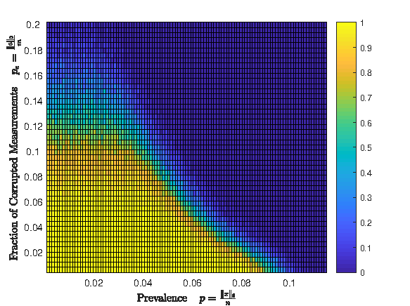
We see that as guaranteed by [25]*Theorem 4.5 for $p=\frac{\left\|\mathbf{x}\right\|_{0}}{n}\leq\frac{7}{31^{2}}\approx 0.0073$ and $p_{e}=0$, the recovery succeeds. But empirically the recovery also succeeds for $p\leq 0.08$ and $p_{e}=0$, i.e. 10 times higher than guaranteed. This suggests that $k$ and thus $m$ could be reduced and still recover whenever $p\leq 0.02$ for instance, which might be sufficient for a prevalence of $p=0.01$.

Further the NNLAD seems to successfully recover even in the presence of sparse noise, i.e. when $p_{e}$ is small. This is not surprising as the NNLAD minimizes the $\ell_{1}$ norm of all possible noises and $\ell_{1}$-minimization is sparsity promoting [4]. Recovery seems to succeeds whenever $p_{e}\leq 0.06$ and $\frac{4}{3}p_{e}+p\leq 0.08$. This error correcting property gives the NNLAD decoding approach advantages over other compressed sensing decoders in the presence of heavy outliers.

However, the error correcting properties cannot be guaranteed uniformly for all $\mathbf{e}$ with $p_{e}\leq 0.06$. If the noise components are active exactly on the support of a column of $\mathbf{A}$ where the signal $\mathbf{x}$ is non-vanishing, the measurement might corresponds to a different signal with the same support. Hence, recovery might fail as soon as $\left\|\mathbf{e}\right\|_{0}$ is at least as large as the number of non-zero entries in a column of $\mathbf{A}$, in this case $k+1=8$. However, there are $\binom{m}{k+1}=\binom{248}{8}\approx 3.16\cdot 10^{14}$ different possible supports of a $k+1$-sparse noise, but only $n=961$ of those appear as columns of the matrix. Thus, if the noise support is drawn uniformly at random, such an event is highly unlikely. Thus, we see that the NNLAD is empirically correcting more errors than expected.

We have explained how compressed sensing can be used to solve the viral detection problem. It generates a non-adaptive testing procedure. Further, we have presented a construction of design matrices that can be used for classical non-adaptive group testing and compressed sensing based viral detection. The construction requires roughly as many tests as other methods from non-adaptive group testing and can possibly outperform those. Adaptive group testing methods still require less tests but can only be performed sequentially which is a critical problem in a pandemic with an exponential growth rate. We have proposed to use the NNLAD as a compressed sensing decoder, since, compared to other compressed sensing decoders, it is robust against heavy tailed noise and does not requires knowledge of noise level. In particular, it also has certain error correcting properties. Lastly our method also computes the viral load of infected individuals.

Classical, deterministic, non-adaptive group testing often makes use of so called disjunct matrices, defined below.

The classical decoding procedure for a disjunct matrices iterates over all $j\in\left[n\right]$ and, if for all $i\in A^{j}$ the $i$-th test is positive, it declares the $j$-th individual as infected. This process is simple and, if $\mathbf{A}$ is $k$-disjunct and there are no more than $k$ infected individuals, it is guaranteed to find exactly all infected individuals [18]. However, every false negative test will result in at least one individual that is falsely flagged as not infected. Thus, this decoding procedure is incredibly sensitive to noises. There are extensions to these matrices which can tolerate a fixed number of errors by forcing the set $A^{j}\setminus\bigcup_{j^{\prime}\in T}A^{j^{\prime}}$ not only to be non-empty but also sufficiently large [1]. Compressed sensing on the other hand makes use of matrices that have a robust null space property.

If $\mathbf{A}$ has the robust null space property of order $k$ any vector $\mathbf{x}$ with at most $k$ non-zero components can be recovered from $\mathbf{A}\mathbf{x}$ by solving a linear program and, in the presence of noise, the estimation error is bounded by a constant times the norm of the noise [12, Chapter 4].

It is quite suprising that there is a common way to generate $k$-disjunct matrices and matrices which have the robust null space property of order $k$. This was proven in [18, Equation (4)] and [22].

This yields that a lot of test schemes for non-adaptive group testing can already be used with the compressed sensing decoding strategy presented in Section 2. Using this method we cannot improve the amount of tests required directly, but, the compressed sensing decoder we propose is significantly more robust to noise. We will see empirically that the compressed sensing decoder will correctly identify all infected individuals even in the presence of one false negative test, unlike the classical group testing decoder for disjunct matrices.

Note that under the assumptions of the theorem the quantity $\frac{\lambda}{D}$ is one over the mutual coherence of the matrix (after suitable normalization). The mutual coherence is a general tool in compressed sensing and it is known that the order of the null space property has to be at least in the order of one over the mutual coherence [15, Equation (9)]. In the special case of binary matrices this result can be refined to account for a better constant using [22].

We introduce the result [26, Theorem 3.4] with some fixed parameters that we will combine with some binary matrices from [22, Page 3015] that have a high number of ones per column but a small inner product between distinct columns.

We now have the necessary tools to proof the main result.

Suppose we fix a threshold $\epsilon>0$ that identifies infected persons, meaning that the $j$-th person is infected if and only if more than $\epsilon$ viruses are contained in the specimen of the $j$-th person, i.e. if and only if $\mathbf{x}_{j}>\epsilon$. In this case we can identify the infected persons even in the presence of small noise. If $\left\|\mathbf{e}\right\|_{1}<\frac{\epsilon}{4}\left(k+1+k\left(2k+3\right)\left\|\mathbf{A}^{\dagger}\right\|_{1\rightarrow 1}\right)^{-1}$, we get

Since $\mathbf{x}_{j}$ is either greater than $\epsilon$ or zero, we can deduce that $\mathbf{x}_{j}>\epsilon$ happens if and only if $\mathbf{x}^{\#}_{j}>\frac{\epsilon}{2}$. After the tests we could declare that a person is infected if $\mathbf{x}^{\#}_{j}>\frac{\epsilon}{2}$, and healthy if this is not fulfilled. This method would still detect the infected individuals in the presence of small noise.

References

- [1] Rudolf Ahlswede and Harout Aydinian. New construction of error-tolerant pooling designs. In Information Theory, Combinatorics, and Search Theory, pages 534–542. Springer, 2013.
- [2] Bubacarr Bah and Jared Tanner. On the construction of sparse matrices from expander graphs. Frontiers in Applied Mathematics and Statistics, 4:39, 2018.
- [3] R. Berinde, A.C. Gilbert, P. Indyk, H. Karloff, and M.J. Strauss. Combining geometry and combinatorics: A unified approach to sparse signal recovery. In Communication, Control, and Computing, 2008 46th Annual Allerton Conference on, pages 798–805. IEEE, 2008.
- [4] E. J. Candès and T. Tao. Decoding by linear programming. IEEE Trans. Inform. Theory, 51(12):4203–4215, 2005.
- [5] Emmanuel J Candès, Justin Romberg, and Terence Tao. Robust uncertainty principles: Exact signal reconstruction from highly incomplete frequency information. IEEE Transactions on information theory, 52(2):489–509, 2006.
- [6] Albert Cohen, Wolfgang Dahmen, and Ronald DeVore. Compressed sensing and best -term approximation. Journal of the American mathematical society, 22(1):211–231, 2009.
- [7] David L Donoho. Compressed sensing. IEEE Transactions on information theory, 52(4):1289–1306, 2006.
- [8] Robert Dorfman. The detection of defective members of large populations. The Annals of Mathematical Statistics, 14(4):436–440, 1943.
- [9] Dingzhu Du and Frank Hwang. Pooling designs and nonadaptive group testing: important tools for DNA sequencing. World Scientific, 2006.
- [10] A. G. D’yachkov and V. V. Rykov. Bounds on the Length of Disjunctive Codes. Probl. Peredachi Inf., 18(3):7–13, 1982.
- [11] United States Food and Drug Administration. FDA news release: Coronavirus (COVID-19) update: FDA issues first emergency authorization for sample pooling in diagnostic testing.
- [12] Simon Foucart and Holger Rauhut. A Mathematical Introduction to Compressive Sensing. Birkhäuser Basel, 2013.
- [13] Sabyasachi Ghosh, Rishi Agarwal, Mohammad Ali Rehan, Shreya Pathak, Pratyush Agrawal, Yash Gupta, Sarthak Consul, Nimay Gupta, Ritika Goyal, Ajit Rajwade, and Manoj Gopalkrishnan. A compressed sensing approach to group-testing for covid-19 detection. ArXiv, abs/2005.07895, 2020.
- [14] Anna C Gilbert, Mark A Iwen, and Martin J Strauss. Group testing and sparse signal recovery. In 2008 42nd Asilomar Conference on Signals, Systems and Computers, pages 1059–1063. IEEE, 2008.
- [15] R. Gribonval and M. Nielsen. Sparse representations in unions of bases. IEEE Transactions on Information Theory, 49(12):3320–3325, Dec 2003.
- [16] Venkatesan Guruswami, Christopher Umans, and Salil Vadhan. Unbalanced expanders and randomness extractors from parvaresh–vardy codes. J. ACM, 56(4), July 2009.
- [17] F. K. Hwang. A method for detecting all defective members in a population by group testing. Journal of the American Statistical Association, 67(339):605–608, 1972.
- [18] W. Kautz and R. Singleton. Nonrandom binary superimposed codes. IEEE Transactions on Information Theory, 10(4):363–377, 1964.
- [19] R. Kueng and P. Jung. Robust nonnegative sparse recovery and the nullspace property of 0/1 measurements. IEEE Transactions on Information Theory, 64(2):689–703, 2018.
- [20] J. N. Laska, M. A. Davenport, and R. G. Baraniuk. Exact signal recovery from sparsely corrupted measurements through the Pursuit of Justice. In 2009 Conference Record of the Forty-Third Asilomar Conference on Signals, Systems and Computers, pages 1556–1560, 2009.
- [21] X. Liu and S. Xia. Reconstruction guarantee analysis of binary measurement matrices based on girth. In 2013 IEEE International Symposium on Information Theory, pages 474–478, 2013.
- [22] Mahsa Lotfi and Mathukumalli Vidyasagar. Compressed sensing using binary matrices of nearly optimal dimensions. IEEE Transactions on Signal Processing, 68:3008–3021, 2020.
- [23] Leon Mutesa, Pacifique Ndishimye, Yvan Butera, Jacob Souopgui, Annette Uwineza, Robert Rutayisire, Emile Musoni, Nadine Rujeni, Thierry Nyatanyi, Edouard Ntagwabira, Muhammed Semakula, Clarisse Musanabaganwa, Daniel Nyamwasa, Maurice Ndashimye, Eva Ujeneza, Ivan Emile Mwikarago, Claude Mambo Muvunyi, Jean Baptiste Mazarati, Sabin Nsanzimana, Neil Turok, and Wilfred Ndifon. A strategy for finding people infected with sars-cov-2: optimizing pooled testing at low prevalence. medRxiv, 2020.
- [24] Hendrik Bernd Petersen, Shankar Agarwal, Peter Jung, and Bubacarr Bah. Improving the reliability of pooled testing with combinatorial decoding and compressed sensing. In 2021 55th Annual Conference on Information Sciences and Systems (CISS), pages 1–5. IEEE, 2021.
- [25] Hendrik Bernd Petersen, Bubacarr Bah, and Peter Jung. Practical high-throughput, non-adaptive and noise-robust sars-cov-2 testing. arXiv preprint arXiv:2007.09171, 2020.
- [26] Hendrik Bernd Petersen, Bubacarr Bah, and Peter Jung. Efficient tuning-free -regression of nonnegative compressible signals. Frontiers in Applied Mathematics and Statistics, 7:615573, 2021.
- [27] Hendrik Bernd Petersen and Peter Jung. Robust instance-optimal recovery of sparse signals at unknown noise levels. Information and Inference: A Journal of the IMA, 11(3):845–887, 2022.
- [28] RM Phatarfod and Aidan Sudbury. The use of a square array scheme in blood testing. Statistics in medicine, 13(22):2337–2343, 1994.
- [29] Jan H Schefe, Kerstin E Lehmann, Ivo R Buschmann, Thomas Unger, and Heiko Funke-Kaiser. Quantitative real-time RT-PCR data analysis: current concepts and the novel “gene expression’s CT difference” formula. Journal of molecular medicine, 84(11):901–910, 2006.
- [30] Michael Schmidt, Sebastian Hoehl, Annemarie Berger, Heinz Zeichhardt, Kai Hourfar, Sandra Ciesek, and Erhard Seifried. FACT-Frankfurt adjusted COVID-19 testing-a novel method enables high-throughput SARS-CoV-2 screening without loss of sensitivity. medRxiv, pages 2020–04, 2020.
- [31] Claudio M Verdun, Tim Fuchs, Pavol Harar, Dennis Elbrächter, David S Fischer, Julius Berner, Philipp Grohs, Fabian J Theis, and Felix Krahmer. Group testing for sars-cov-2 allows for up to 10-fold efficiency increase across realistic scenarios and testing strategies. Frontiers in Public Health, 9:583377, 2021.
- [32] Junan Zhu, Kristina Rivera, and Dror Baron. Noisy Pooled PCR for Virus Testing. bioRxiv, 2020.